1. Introduction

2. Problem Formulation

3. Proposed Method

Figure 1. Proces Phase Framework

Figure 1. Proces Phase Framework

3.1. Feature Selection and Decision-Making in Random Forests

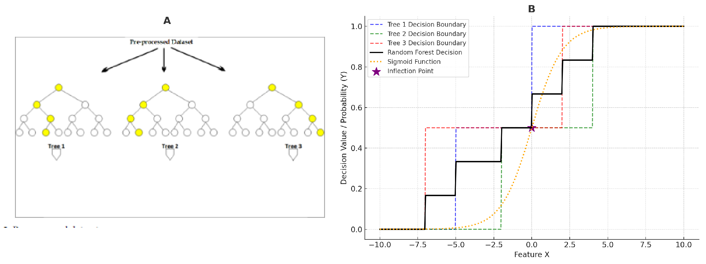
The process begins with the feature selection phase, where the dataset undergoes a thorough preprocessing stage, as shown in Figure A of the combined visualization. Here, the preprocessed dataset is passed into multiple decision trees (Tree 1, Tree 2, and Tree 3), each of which independently evaluates the importance of different features. This process involves data cleaning, handling missing values, and addressing inconsistencies to ensure the dataset is suitable for model training.

Within this ensemble of decision trees, each feature $x_i$ contributes differently to the decision-making process, and the importance of these features is evaluated at each split within the trees. The concept of a "cave degree" operator is introduced to measure the relevance of each feature based on its contribution to reducing impurity at the nodes of the decision trees. Let $C_i$ represent the cave degree of feature $x_i$, which is computed by averaging the importance scores $\mathrm{Importance}(x_i,t)$ across all trees in the Random Forest ensemble:

$$C_i={\displaystyle \frac{1}{n_{\mathrm{trees}}}}\sum _{t=1}^{n_{\mathrm{trees}}}\mathrm{Importance}(x_i,t)$$

The cave degree captures how much a feature contributes to the model’s predictive performance, and features with higher cave degrees are considered more significant for the overall decision-making process.

In Figure A, the decision trees visually highlight key decision nodes (yellow circles), representing where significant feature-based decisions are made within each tree. These nodes signify the points where features with higher cave degrees are actively influencing the tree’s decisions.

Moving to Figure B, we observe the aggregated output of the Random Forest model, where the individual decisions from Tree 1, Tree 2, and Tree 3 are combined to form a unified decision boundary. The dashed lines in different colors (blue, green, and red) represent the decision boundaries of each individual tree. The solid black line shows the overall decision boundary of the Random Forest model, which is the average of the decisions made by all trees, demonstrating the ensemble’s ability to create a more robust and accurate predictive model.

The orange dotted line represents the sigmoid function $S\left(x\right)={\displaystyle \frac{1}{1+e^{-x}}}$, which converts the combined output of the decision trees into a smooth probabilistic prediction ranging between 0 and 1. The sigmoid function plays a crucial role in transforming the raw decision outputs into probabilities, making the model suitable for classification tasks where outputs are interpreted as probabilities of belonging to a particular class.

An important aspect of this visualization is the inflection point marked by the purple star on the graph in Figure B. This point corresponds to $x=0$ on the sigmoid function, indicating where the probability shifts most rapidly. It signifies the threshold where the model’s confidence in the prediction changes most dramatically, thus serving as a critical decision boundary in classification tasks.

Therefore, by applying the cave degree operator and incorporating the sigmoid transformation, the Random Forest model efficiently selects and weights the most relevant features, leading to improved accuracy and robustness in its predictions. This is further validated by the combined decision boundaries shown in Figure B, where the ensemble of decision trees collectively contributes to a refined, probability-based prediction output.

Figure 2. (A) Preprocessed Dataset Feeding into Random Forest Decision Trees; (B) Combined Decision Boundaries with Sigmoid Function and Inflection Point

Figure 2. (A) Preprocessed Dataset Feeding into Random Forest Decision Trees; (B) Combined Decision Boundaries with Sigmoid Function and Inflection Point

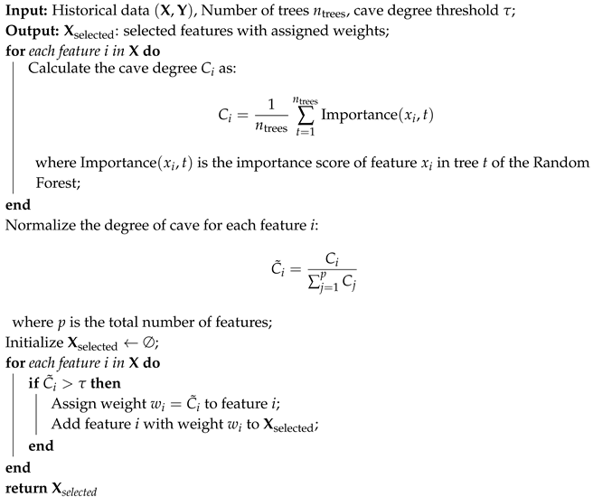
As depicted in Algorithm 1, the feature selection process in a Random Forest is guided by the cave degree values. By assigning weights to features based on their normalized cave degrees,

$${\tilde{C}}_i={\displaystyle \frac{C_i}{{\sum }_{j=1}^p{C}_j}},$$

where p is the total number of features, the Random Forest model prioritizes the most relevant features. This ultimately enhances the model’s predictive power, as the most important features are given more weight, leading to superior performance in both classification and regression tasks.

Algorithm 1: Feature Selection Using cave Degree in Random Forest

$$C_i={\displaystyle \frac{1}{n_{\mathrm{trees}}}}\sum _{t=1}^{n_{\mathrm{trees}}}\mathrm{Importance}(x_i,t),$$

where $n_{\mathrm{trees}}$ is the total number of trees in the ensemble. To normalize the cave degrees, we use:

$${\tilde{C}}_i={\displaystyle \frac{C_i}{{\sum }_{j=1}^p{C}_j}},$$

where ${\tilde{C}}_i$ is the normalized cave degree of feature $x_i$, and p is the total number of features. This normalization ensures that the cave degrees are on a comparable scale. Features with a normalized cave degree ${\tilde{C}}_i$ above a certain threshold $\tau$ are selected, as they are considered the most relevant to predict customer churn. A higher cave degree indicates a greater importance of the feature, making it a better candidate for inclusion in the predictive model.

3.2. Optimization Phase

This section introduces the second phase of the optimization process, which involves employing two well-known metaheuristic algorithms. Adaptive Large Neighborhood Search (ALNS) and Particle Swarm Optimization (PSO). To further enhance the optimization process, we propose a novel strategy called the Magnetic Force Perturbation Technique inspired by the natural behavior of magnetic fields, where forces attract or repel particles depending on their polarities. This phenomenon can be modeled mathematically using Coulomb’s law for electric forces or the law of magnetic interaction. Analogously, in optimization, we simulate these forces to guide the exploration of the solution space. If we denote the current solution by $\mathbf{x}$ and potential solutions by $\mathbf{y}$, the force ${\mathbf{F}}_{xy}$ exerted on $\mathbf{x}$ by $\mathbf{y}$ can be expressed as:

$${\mathbf{F}}_{xy}=k{\displaystyle \frac{q_x{q}_y}{{\parallel \mathbf{y}-\mathbf{x}\parallel }^2}}$$

where k is a constant, $q_x$ and $q_y$ represent the "charges" or qualities of solutions $\mathbf{x}$ and $\mathbf{y}$ respectively, and $\parallel \mathbf{y}-\mathbf{x}\parallel$ is the Euclidean distance between the solutions. Solutions $\mathbf{x}$ close to promising regions, which have higher quality (or "charge"), experience an attraction force pulling them towards those regions. In contrast, solutions in less favorable regions experience repulsion.

The perturbation applied to the current solution $\mathbf{x}$ is based on the calculated forces. Let $\mathbf{P}\left(\mathbf{x}\right)$ represent the perturbation applied to $\mathbf{x}$. The perturbation is a function of the force ${\mathbf{F}}_{xy}$ and can be defined as:

$$\mathbf{P}\left(\mathbf{x}\right)=\alpha {\mathbf{F}}_{xy}$$

where $\alpha$ is a control parameter that modulates the magnitude of the perturbation. Larger perturbations explore new regions of the solution space, while smaller perturbations refine solutions in promising areas.

The optimization process is iterative. In each iteration, the solutions are adjusted based on the simulated magnetic forces. If we denote the state of the search process at iteration t by ${\mathbf{x}}_t$, the updated solution ${\mathbf{x}}_{t+1}$ is given by:

$${\mathbf{x}}_{t+1}={\mathbf{x}}_t+\mathbf{P}\left({\mathbf{x}}_t\right)$$

The forces ${\mathbf{F}}_{xy}$ can be adapted based on the search progress. For instance, as the algorithm converges, the forces might be adjusted to focus more on local refinement or global exploration depending on the current state of the search, adapting the parameter $\alpha$ accordingly. This dynamic adjustment helps in balancing exploration of new areas with exploitation of known promising regions, thus improving the efficiency of the optimization process.

3.2.1. Adaptive Large Neighborhood Search (ALNS) Algorithm

Adaptive Large Neighborhood Search (ALNS) is a powerful metaheuristic optimization technique designed to tackle complex combinatorial problems. The core idea behind ALNS is to iteratively explore large neighborhoods of the current solution by applying various perturbation and repair strategies. This allows the algorithm to escape local optima and efficiently search through a broader solution space. ALNS adapts its neighborhood structures based on the observed performance, dynamically balancing exploration and exploitation throughout the search process.

In this context, ALNS is utilized to address the problem of churn prediction by optimizing feature selection. By incorporating advanced techniques such as magnetic force perturbation and strategic solution modifications (i.e., break and repair), ALNS can enhance the search for the most effective feature subsets. The magnetic force perturbation guides the search process by simulating forces that attract or repel solutions based on their quality, thereby improving the exploration of promising regions and avoiding less favorable ones. The following algorithm presents the integration of ALNS with magnetic force perturbation and break/repair strategies, specifically tailored to optimize feature selection for churn prediction and achieve the best performance metrics.

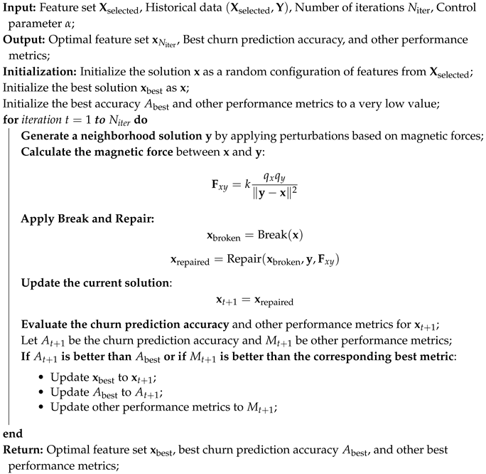
Algorithm 2 starts by initializing the solution $\mathbf{x}$ as a random configuration of features selected from ${\mathbf{X}}_{\mathrm{selected}}$. Additionally, the algorithm sets ${\mathbf{x}}_{\mathrm{best}}$ to the initial solution $\mathbf{x}$ and initializes the best churn prediction accuracy $A_{\mathrm{best}}$ and other performance metrics to very low values.

For each iteration t from 1 to $N_{\mathrm{iter}}$, the algorithm generates a neighborhood solution $\mathbf{y}$ by applying perturbations based on magnetic forces. The magnetic force ${\mathbf{F}}_{xy}$ between the current solution $\mathbf{x}$ and the neighborhood solution $\mathbf{y}$ is computed as:

$${\mathbf{F}}_{xy}=k{\displaystyle \frac{q_x{q}_y}{{\parallel \mathbf{y}-\mathbf{x}\parallel }^2}}$$

where k is a constant, and $q_x$ and $q_y$ represent the "charges" or qualities of solutions $\mathbf{x}$ and $\mathbf{y}$, respectively.

The algorithm then applies the "break" and "repair" strategies to the current solution $\mathbf{x}$. The "break" strategy creates a modified solution ${\mathbf{x}}_{\mathrm{broken}}$ by removing or altering parts of $\mathbf{x}$:

$${\mathbf{x}}_{\mathrm{broken}}=\mathrm{Break}\left(\mathbf{x}\right)$$

The "repair" strategy then adjusts ${\mathbf{x}}_{\mathrm{broken}}$ using the neighborhood solution $\mathbf{y}$ and the magnetic force ${\mathbf{F}}_{xy}$ to produce a repaired solution:

$${\mathbf{x}}_{\mathrm{repaired}}=\mathrm{Repair}({\mathbf{x}}_{\mathrm{broken}},\mathbf{y},{\mathbf{F}}_{xy})$$

The updated solution is then set to:

$${\mathbf{x}}_{t+1}={\mathbf{x}}_{\mathrm{repaired}}$$

The algorithm evaluates the churn prediction accuracy $A_{t+1}$ and other performance metrics $M_{t+1}$ for the updated solution ${\mathbf{x}}_{t+1}$. If the accuracy $A_{t+1}$ exceeds the previously recorded best accuracy $A_{\mathrm{best}}$, or if $M_{t+1}$ shows improvement over the best recorded metrics, the algorithm updates ${\mathbf{x}}_{\mathrm{best}}$ to ${\mathbf{x}}_{t+1}$, and sets $A_{\mathrm{best}}$ and the other metrics to $A_{t+1}$ and $M_{t+1}$, respectively.

After completing all iterations, the algorithm returns the best solution ${\mathbf{x}}_{\mathrm{best}}$, along with the corresponding best churn prediction accuracy $A_{\mathrm{best}}$ and other performance metrics.

Algorithm 2: Optimization Using ALNS with Magnetic Force Perturbation

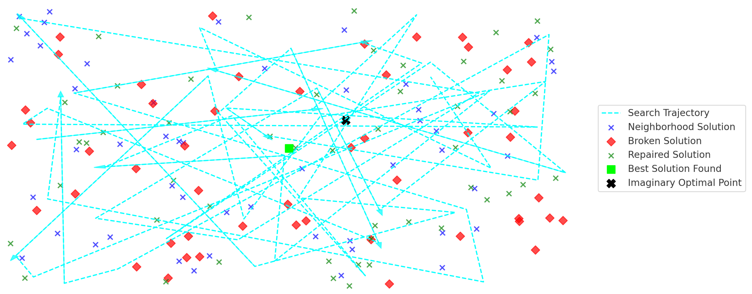
Figure 3. ALNS search trajectory within a solution space. This figure represents the search trajectory of the ALNS algorithm through the solution space. The blue lines with arrows indicate the path taken by the algorithm in navigating from one solution to another. The red, blue, and green points correspond to different evaluated solutions, where red indicates potential solutions, blue represents neighborhood solutions, and green signifies the best or final solutions found. The black star marks the optimal or most favorable solution identified during the search process, showcasing how ALNS dynamically explores and exploits the solution space.

Figure 3. ALNS search trajectory within a solution space. This figure represents the search trajectory of the ALNS algorithm through the solution space. The blue lines with arrows indicate the path taken by the algorithm in navigating from one solution to another. The red, blue, and green points correspond to different evaluated solutions, where red indicates potential solutions, blue represents neighborhood solutions, and green signifies the best or final solutions found. The black star marks the optimal or most favorable solution identified during the search process, showcasing how ALNS dynamically explores and exploits the solution space.

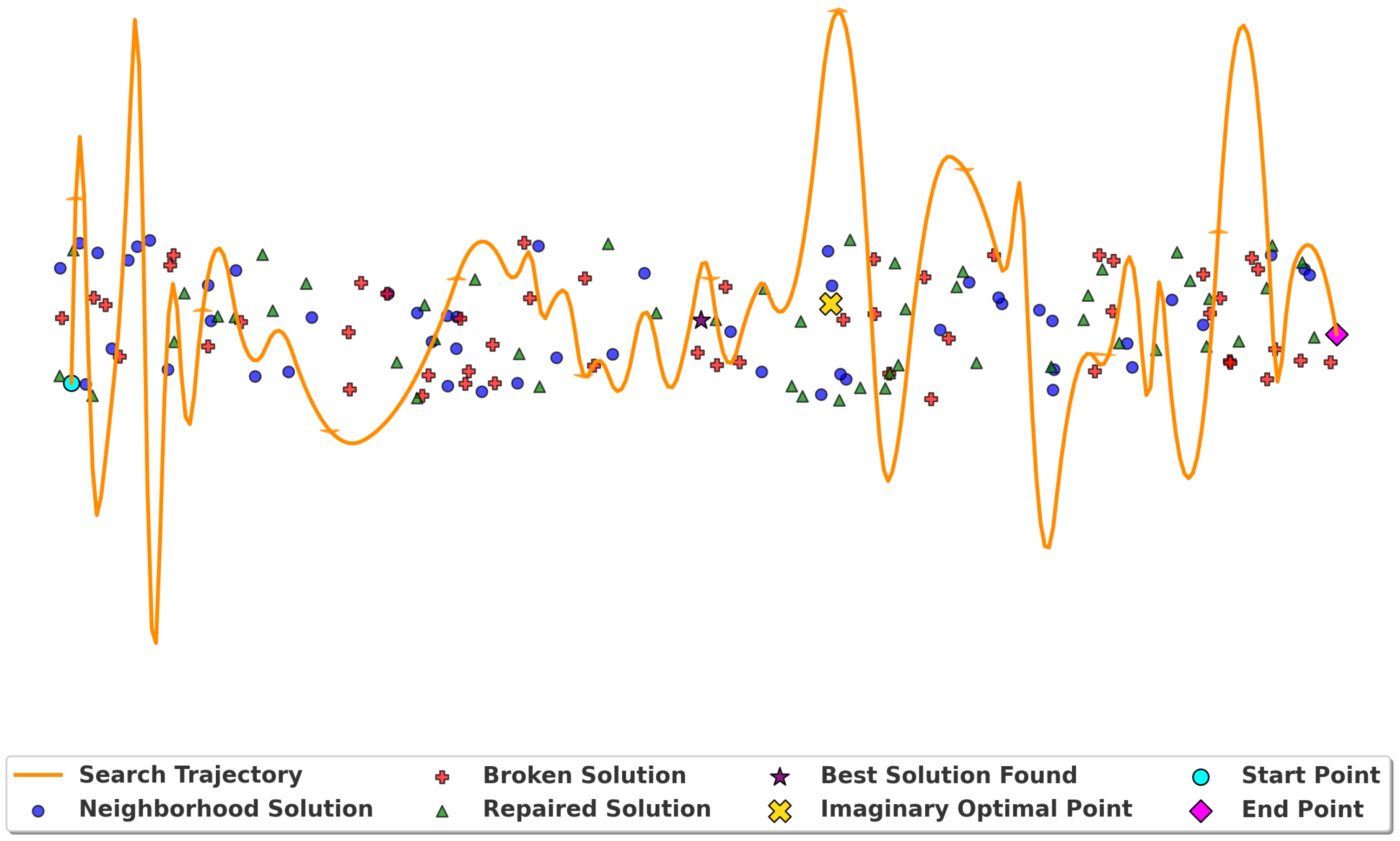
Figure 4. Optimized ALNS Path Exploration with Distinct Solution Mapping. This figure illustrates the trend of a performance metric over iterations or time steps as the ALNS algorithm progresses. The orange line represents the smoothed trend of the metric being tracked, while the colored points indicate individual data points at each step, iteration, or trial. The peaks and troughs in the line show periods of high and low performance, respectively, reflecting the oscillatory and converging behavior of the algorithm as it seeks optimal solutions.

Figure 4. Optimized ALNS Path Exploration with Distinct Solution Mapping. This figure illustrates the trend of a performance metric over iterations or time steps as the ALNS algorithm progresses. The orange line represents the smoothed trend of the metric being tracked, while the colored points indicate individual data points at each step, iteration, or trial. The peaks and troughs in the line show periods of high and low performance, respectively, reflecting the oscillatory and converging behavior of the algorithm as it seeks optimal solutions.

3.2.2. Particle Swarm Optimization Algorithm (PSO)

Particle Swarm Optimization (PSO) is a computational method inspired by the social behavior of birds and fish. Developed by Kennedy and Eberhart in 1995 [41], PSO is a heuristic optimization technique that simulates the social interaction of a swarm of particles in a search space to find optimal solutions to complex problems. In PSO, each particle represents a potential solution and moves through the search space influenced by its own experience and that of its neighbors. Particles adjust their positions based on their own best-known position and the best-known positions of the swarm, guided by a velocity update mechanism. This process continues iteratively, with particles converging towards the optimal solution over time.

As shown in Algorithm 3, the PSO algorithm begins with initializing a set of particles, where each particle i is represented by a feature configuration ${\mathbf{x}}_i$ selected from the set ${\mathbf{X}}_{\mathrm{selected}}$. Each particle has an associated velocity ${\mathbf{v}}_i$, and the personal best solution ${\mathbf{x}}_{i,\mathrm{pbest}}$ is initialized to ${\mathbf{x}}_i$. The global best solution ${\mathbf{x}}_{\mathrm{gbest}}$ is set to the best personal best among all particles. The best accuracy $A_{\mathrm{best}}$ and other performance metrics are initialized to very low values.

For each iteration t from 1 to $N_{\mathrm{iter}}$, the algorithm updates the velocity and position of each particle. The velocity ${\mathbf{v}}_{i,t+1}$ of particle i is updated based on its previous velocity, its distance from its personal best ${\mathbf{x}}_{i,\mathrm{pbest}}$, and its distance from the global best ${\mathbf{x}}_{\mathrm{gbest}}$:

$${\mathbf{v}}_{i,t+1}=\mathbf{w}{\mathbf{v}}_{i,t}+c_1{r}_1({\mathbf{x}}_{i,\mathrm{pbest}}-{\mathbf{x}}_i)+c_2{r}_2({\mathbf{x}}_{\mathrm{gbest}}-{\mathbf{x}}_i)$$

where $\mathbf{w}$ is the inertia weight, $c_1$ and $c_2$ are cognitive and social coefficients, and $r_1$ and $r_2$ are random numbers uniformly distributed in the range $[0,1]$. The position ${\mathbf{x}}_{i,t+1}$ of the particle is then updated using:

$${\mathbf{x}}_{i,t+1}={\mathbf{x}}_i+{\mathbf{v}}_{i,t+1}$$

Following the velocity and position update, the algorithm applies magnetic force perturbation. The magnetic force ${\mathbf{F}}_{i,\mathrm{gbest}}$ between the current position of the particle i and the global best position ${\mathbf{x}}_{\mathrm{gbest}}$ is calculated as:

$${\mathbf{F}}_{i,\mathrm{gbest}}=k{\displaystyle \frac{q_i{q}_{\mathrm{gbest}}}{\parallel {\mathbf{x}}_{\mathrm{gbest}}-{\mathbf{x}}_i{\parallel }^2}}$$

where k is a constant and $q_i$ and $q_{\mathrm{gbest}}$ represent the "charges" of the particle and the global best solution, respectively. The perturbation applied to the position of the particle is:

$${\mathbf{x}}_{i,\mathrm{perturbed}}={\mathbf{x}}_{i,t+1}+\alpha {\mathbf{F}}_{i,\mathrm{gbest}}$$

where $\alpha$ is a control parameter that scales the magnetic force effect.

The perturbed solution ${\mathbf{x}}_{i,\mathrm{perturbed}}$ is then evaluated for churn prediction accuracy $A_{i,t+1}$ and other performance metrics $M_{i,t+1}$. If this evaluation yields better performance metrics compared to the current personal best, the personal best solution ${\mathbf{x}}_{i,\mathrm{pbest}}$ is updated to ${\mathbf{x}}_{i,\mathrm{perturbed}}$, and the corresponding accuracy and metrics are updated. Furthermore, if the accuracy $A_{i,t+1}$ for any particle surpasses the global best accuracy $A_{\mathrm{best}}$, the global best solution ${\mathbf{x}}_{\mathrm{gbest}}$ is updated to this particle’s personal best. This ensures that the global best solution reflects the highest accuracy and best performance metrics found across all particles. After completing all iterations, the algorithm returns the global best feature set ${\mathbf{x}}_{\mathrm{gbest}}$, along with the highest accuracy $A_{\mathrm{best}}$ and other performance metrics achieved.

Algorithm 3: Particle Swarm Optimization with Magnetic Force Perturbation

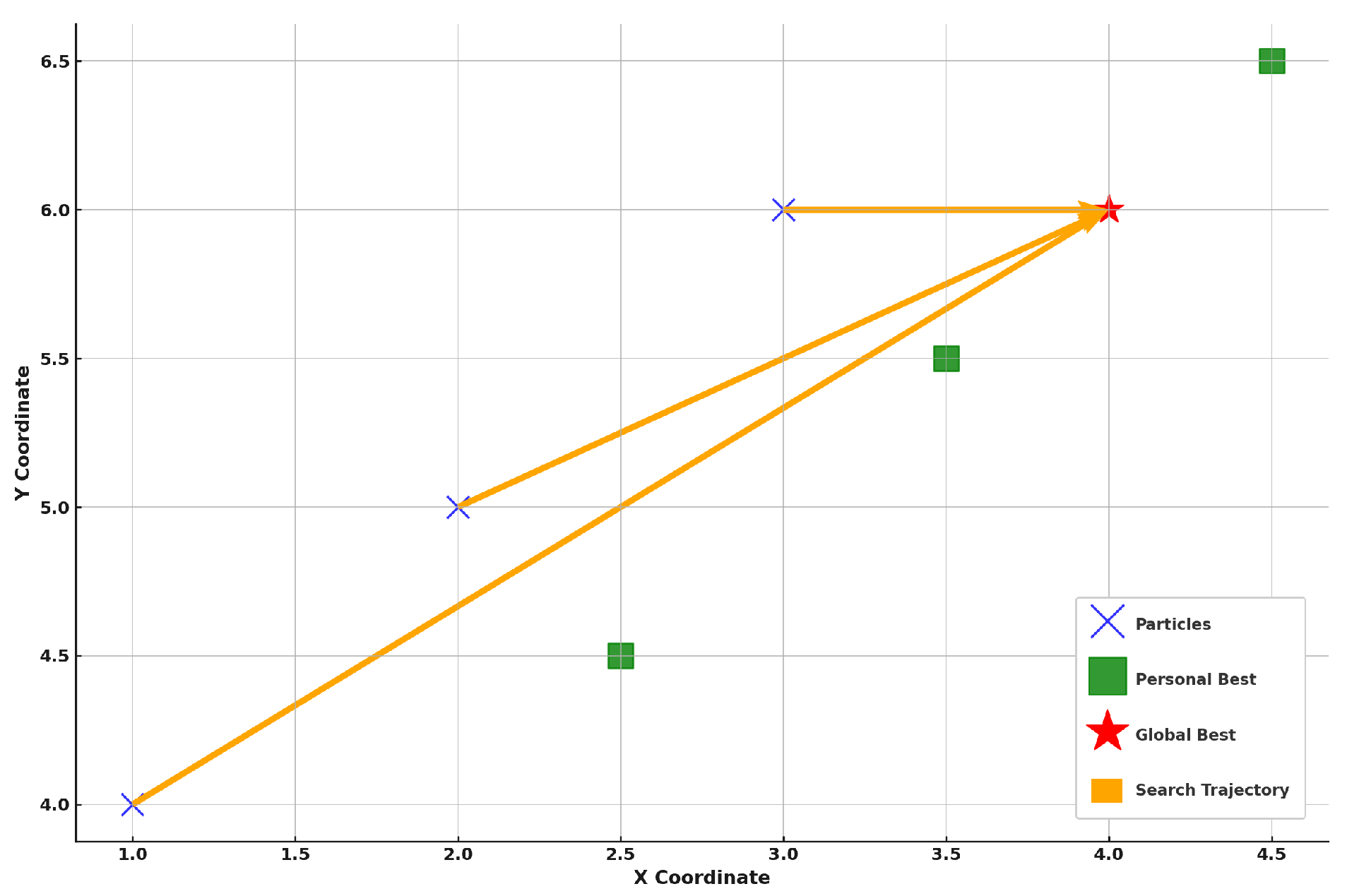
Figure 5. PSO virtual exploration. This figure illustrates the virtual exploration of the Particle Swarm Optimization (PSO) algorithm within the solution space. The blue ’X’ markers represent the positions of particles within the search space at a given time, while the green squares indicate the personal best positions identified by each particle based on their experience. The red star signifies the global best solution identified by the swarm, which represents the optimal solution found thus far. The orange lines represent the search trajectories of particles, showing how they are influenced by both their personal bests and the global best. This diagram captures the dynamic interplay between individual particle exploration and the collective movement towards the global optimum as the algorithm progresses.

Figure 5. PSO virtual exploration. This figure illustrates the virtual exploration of the Particle Swarm Optimization (PSO) algorithm within the solution space. The blue ’X’ markers represent the positions of particles within the search space at a given time, while the green squares indicate the personal best positions identified by each particle based on their experience. The red star signifies the global best solution identified by the swarm, which represents the optimal solution found thus far. The orange lines represent the search trajectories of particles, showing how they are influenced by both their personal bests and the global best. This diagram captures the dynamic interplay between individual particle exploration and the collective movement towards the global optimum as the algorithm progresses.

4. Computational Experiment

4.1. Computational Experimental Results with Azani Auto Insurance Company

This section presents the computational experimental results derived from the Azani Auto Insurance Company database, which was analyzed using various state-of-the-art machine learning techniques such as XGBoost, Random Forest, and SVM, providing a comprehensive performance comparison. The results from these machine learning models were benchmarked against our proposed metaheuristic methods: ARALFO and ARFPSO. Table 2. The comparison reveals that ARALFO outperforms the other methods across key metrics, including Accuracy, Precision, Recall, and F1 Score, demonstrating a well-rounded and effective approach. While Random Forest and XGBoost also show strong performance, particularly in Precision, ARALFO achieves a better balance across all metrics.

The results presented in Table 2 offer a comprehensive comparison of the predictive performance of different machine learning models on the Azani dataset. Among the models, the ARALFO method demonstrates the highest overall performance, with an accuracy of 0.95, which translates to an error rate of only 0.05. This indicates a superior ability to correctly predict outcomes compared to the other models. Furthermore, ARALFO also achieves the highest F1 score (0.95), reflecting balanced performance between precision (0.95) and recall (0.94), making it the most reliable model for handling false positives and false negatives effectively.

In comparison, the Random Forest model, while still performing well with an accuracy of 0.90, shows a slightly higher error rate of 0.10. Its F1 Score matches its precision at 0.91, indicating that although it makes accurate predictions, it is slightly less consistent in retrieving all relevant instances compared to ARALFO. The Kappa statistic for Random Forest (0.85) suggests substantial agreement, but it does not reach the level of agreement seen with ARALFO (Kappa = 0.92). This implies that while Random Forest is a robust model, ARALFO outperforms it in handling class imbalances and making accurate predictions beyond mere chance.

The XGBoost model, with an accuracy of 0.88 and an error rate of 0.12, ranks third in performance. It maintains a relatively high precision (0.90) and recall (0.88), resulting in a commendable F1 Score of 0.89. However, the lower Kappa value of 0.83 indicates that XGBoost has a lower level of reliability compared to the ARALFO and Random Forest models. The AUC value of 0.90 for XGBoost is also slightly less than the others, indicating it has a marginally lower ability to distinguish between positive and negative classes.

ARFPSO, while achieving an accuracy of 0.93 and an error rate of 0.07, has an F1 Score of 0.90, which is slightly lower than expected given its accuracy. This discrepancy can be attributed to the balance between precision (0.91) and recall (0.92). The Kappa statistic of 0.89 and AUC of 0.94 indicate that ARFPSO performs well overall but does not surpass the consistency and reliability demonstrated by ARALFO.

The Sensitivity (Recall) and Specificity metrics further highlight the models’ capabilities. ARALFO’s specificity of 0.96 means it has the highest ability to correctly identify true negatives, making it highly effective at distinguishing non-churn cases. In contrast, XGBoost, despite having a relatively high recall (0.88), exhibits the lowest specificity (0.89), suggesting that it is less effective in identifying true negatives compared to the other models.

In summary, the analysis reveals that ARALFO is the most effective model for the Azani data set, excelling in all key metrics, including precision, precision, recall, F1 Score, Kappa and AUC. The Random Forest model also performs well, but its slightly lower Kappa and F1 Score indicate that it is less consistent in handling class imbalances. ARFPSO is a strong contender with high accuracy and AUC, but it falls short of ARALFO’s overall performance. The XGBoost model, while still effective, shows the least reliability among the four models, making it less suitable for scenarios that require high precision and recall. These results highlight the importance of evaluating multiple metrics to gain a complete understanding of model performance and select the most appropriate model to predict churn in this dataset.

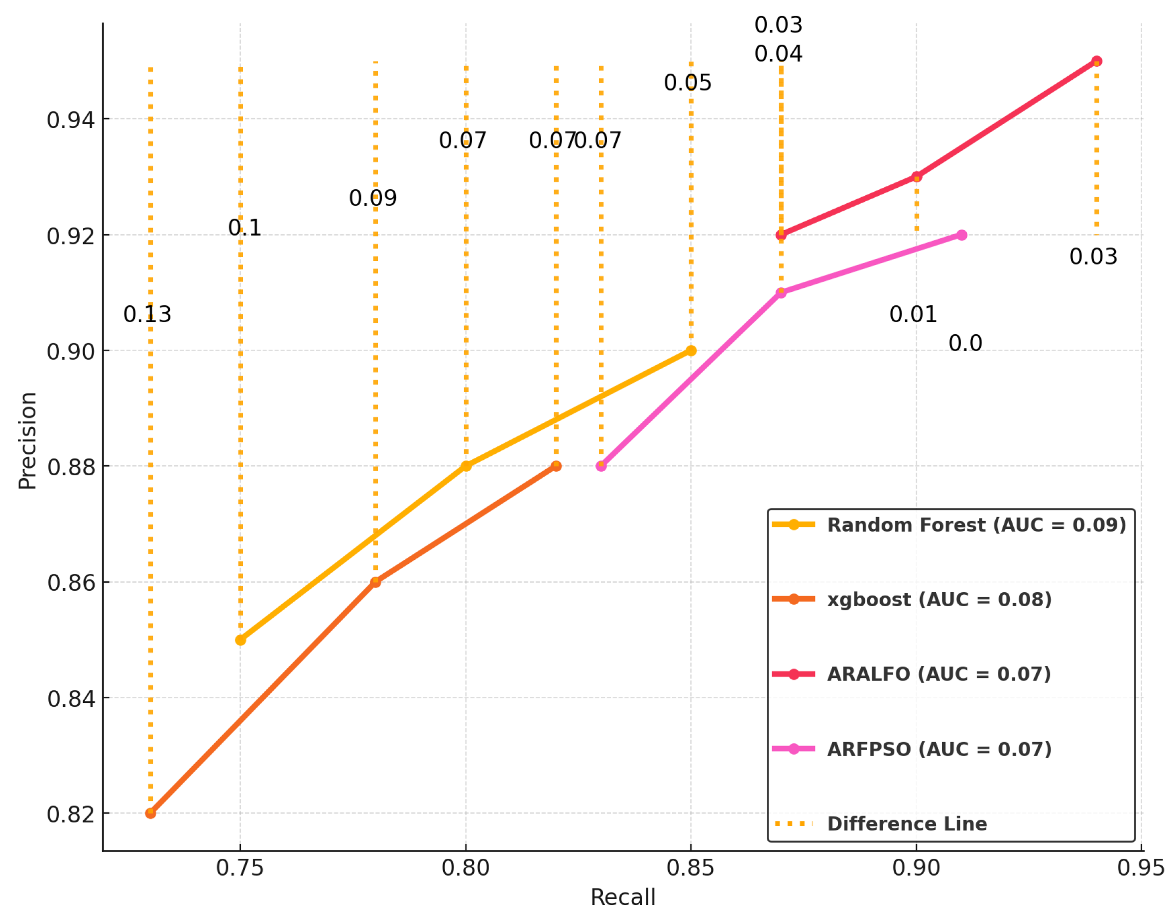
Figure 6. Precision-Recall Curve Analysis

Figure 6. Precision-Recall Curve Analysis

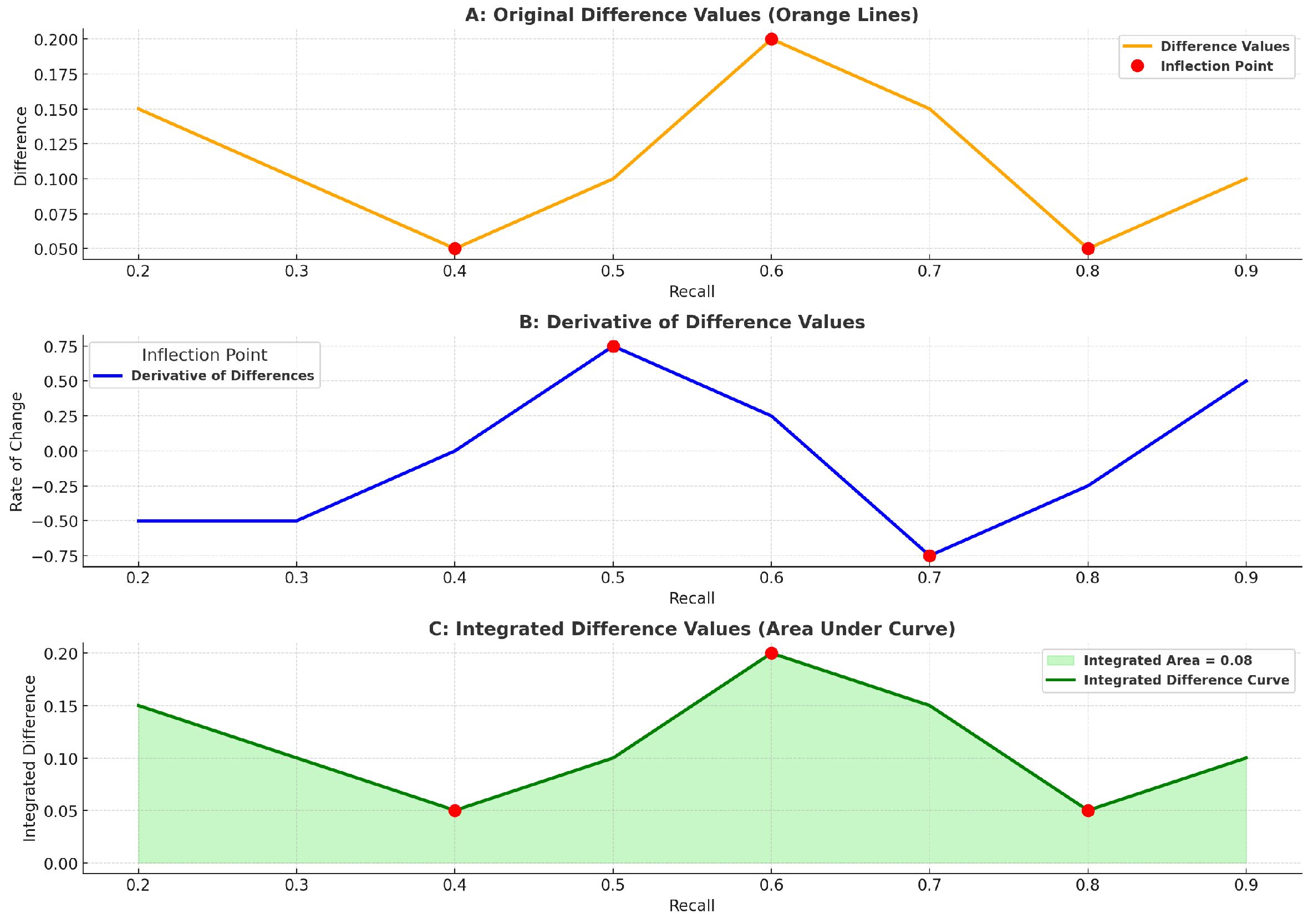
Figure 7. Integrated Difference Values (Area Under Curve)

Figure 7. Integrated Difference Values (Area Under Curve)

Figure 8 employs a precision-recall curve to showcase the comparative performance of multiple models (Random Forest, XGBoost, ARALFO, and ARFPSO). The use of orange dotted lines and exact numerical differences between the curves offers a nuanced understanding of how much one model outperforms another at each recall level. This added layer of detail is particularly valuable, as it reveals not just which model is better but quantifies the margin of improvement or lag, making the differences transparent and measurable. ARALFO’s consistent precision across varying recall levels stands out, demonstrating its reliability in maintaining high performance. This reliability suggests that ARALFO would be a practical choice for tasks where precision at different recall thresholds is paramount.

Figure 7 provides a deeper analysis derived from the original precision-recall curve from Figure 8. Graph A captures the absolute differences between the models, identifying key inflection points where performance changes occur. In contrast, graph B delves deeper by calculating the rate of change (derivative), showing how quickly these differences evolve, which pinpoints the specific recall levels where models either diverge or converge in performance. This transition from Graph A to Graph B reveals the dynamics of model behavior, offering a more detailed view of where ARALFO stands out or where others begin to falter. Graph C then integrates these differences into the recall range, providing a cumulative view of the overall performance disparity among the models. Together, these graphs illustrate both the static and dynamic aspects of model differences, with ARALFO consistently demonstrating stability and adaptability, making it a reliable choice for tasks that demand consistent precision across varying recall values. This comprehensive analysis emphasizes why ARALFO has an edge, particularly in scenarios where maintaining a performance balance is crucial.

4.2. Performance Comparison Using Josep Lledó and Jose M. Pavía Dataset [43]

In this section, we conduct an evaluation of our model alongside other state-of-the-art algorithms using the Josep Lledó and Jose M. Pavía dataset, which is based on an actual motor vehicle insurance dataset [43]. This comparison provides insight into how different machine learning models perform on real-world data.

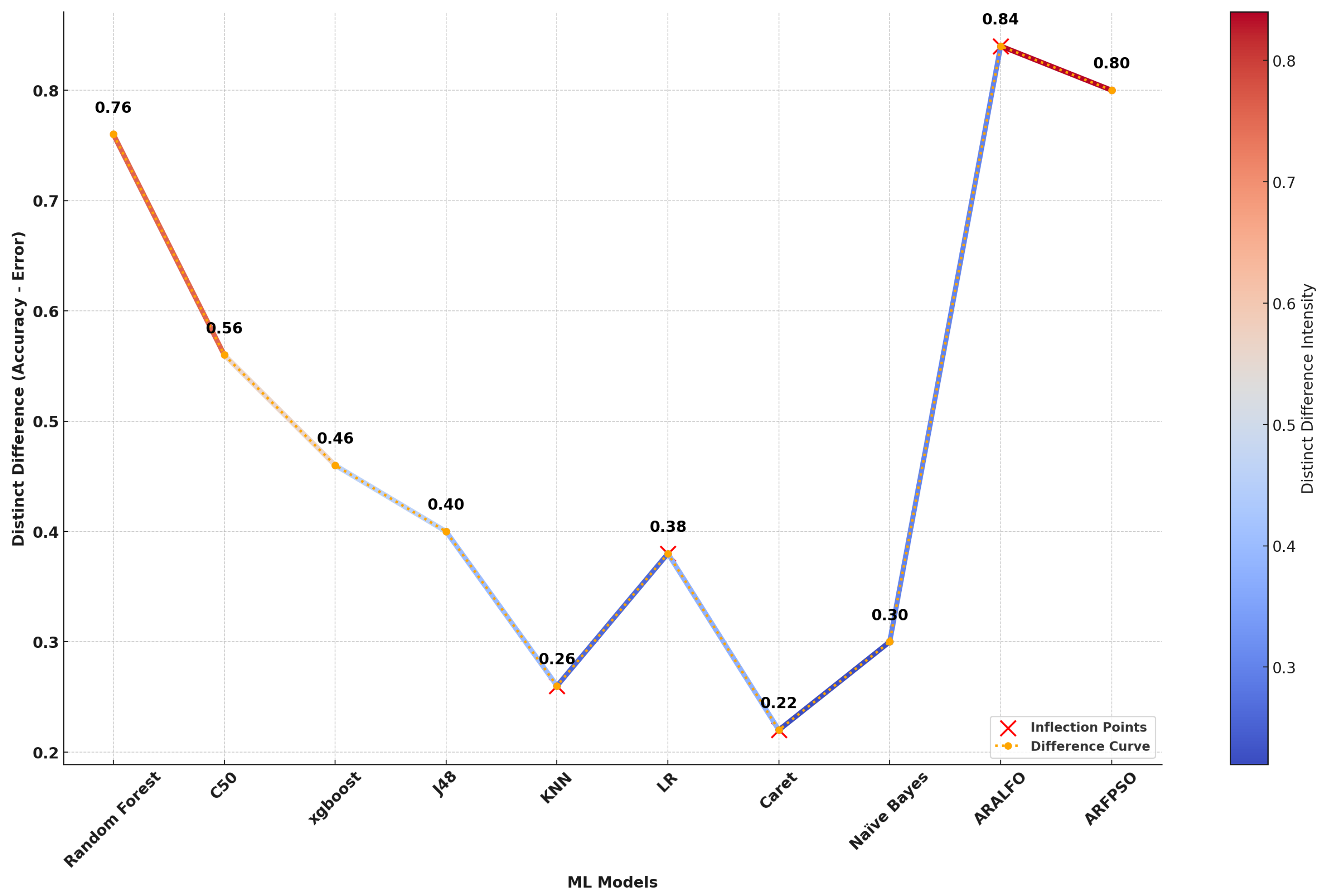
Table 3 illustrates that the ARALFO model consistently outperforms all other models across most evaluation metrics. It achieves the highest Accuracy (0.92), the lowest Error Rate (0.08), and the best Kappa (0.84), indicating a strong level of agreement between predicted and actual classifications. Moreover, ARALFO attains the highest AUC (0.94), showcasing its superior ability to distinguish between different classes.

In recall-related metrics, ARALFO continues to excel with the highest Sensitivity (0.90), demonstrating its effectiveness in correctly identifying positive cases. It also boasts the highest Specificity (0.93), reflecting its outstanding performance in identifying negative cases. Additionally, the model achieves the best Precision (0.91), indicating a low false-positive rate, and attains the highest F1 Score (0.89), which underscores its balanced trade-off between precision and recall.

Although the ARFPSO model shows commendable performance with high values in Accuracy (0.90), Kappa (0.80), AUC (0.92), and other metrics, it consistently ranks slightly below ARALFO in all categories. In contrast, models such as Random Forest and C50 perform moderately, with reasonable accuracy but lower metrics like AUC and Kappa, indicating less reliability in distinguishing between classes.

The remaining models, including KNN, Naïve Bayes, LR, and Caret, exhibit substantially lower performance across all metrics, suggesting they are less suited for tasks requiring high precision and recall. Overall, the analysis clearly demonstrates that ARALFO is the most robust and reliable model for this dataset, consistently achieving the highest scores across all critical performance metrics.

Figure 8. Distinct Differences in Model Performance

Figure 8. Distinct Differences in Model Performance

4.3. Ablation Experimental Results

In this section, we present the results of ablation experiments designed to assess the impact of two critical components: the cave-degree perturbation (CDP) and the magnetic force perturbation (MFP) on the performance of our proposed model. These experiments were conducted to evaluate how each component contributes to the overall effectiveness of the model, with three distinct configurations analyzed to provide a comprehensive understanding of their individual and combined effects.

In the first experiment, we retained the cave-degree perturbation technique during feature selection, while omitting the magnetic force perturbation technique during optimization. The results showed a notable decrease in accuracy from 0.95 to 0.86, indicating that while cave-degree perturbation positively impacts feature selection, the absence of magnetic force perturbation adversely affects the model’s ability to effectively explore the solution space. The precision also dropped from 0.95 to 0.88, reflecting the negative impact on the model’s ability to correctly identify positive instances. Additionally, recall decreased from 0.93 to 0.79, highlighting a reduced capability to capture true positives without magnetic force perturbation. The F1 score fell from 0.95 to 0.82, demonstrating a less balanced performance between precision and recall due to the removal of magnetic force perturbation.

The second experiment involved applying the magnetic force perturbation technique during optimization while omitting the cave-degree perturbation technique during feature selection. This configuration resulted in a decrease in accuracy from 0.95 to 0.84, suggesting that the removal of cave-degree perturbation negatively affects the quality of feature selection, even though magnetic force perturbation aids in solution space exploration. Precision was reduced from 0.95 to 0.87, indicating that the absence of cave-degree perturbation impacts the model’s ability to minimize false positives. Recall decreased from 0.93 to 0.77, showing a diminished ability to capture true positives when cave-degree perturbation was omitted. The F1 score dropped from 0.95 to 0.80, reflecting a decreased balance between precision and recall.

In the third experiment, both techniques—cave-degree perturbation and magnetic force perturbation—were removed. This configuration resulted in a significant decrease in accuracy to 0.78, which highlights the substantial impact of removing both techniques on the overall accuracy of the model. The precision decreased to 0.73, indicating an increased difficulty in managing false positives without the enhancements provided by both techniques. Recall fell to 0.68, reflecting a reduced ability to identify true positives in the absence of both techniques. The F1 score decreased to 0.70, demonstrating a significant decrease in balanced performance due to the removal of both techniques.

As shown in the tables below, CDT denotes cave-degree perturbation, MFT denotes magnetic force perturbation, and ✓ and × are used to indicate the inclusion or exclusion of each technique, respectively.

Table 4. Adjusted Performance Comparison of ARALFO and ARFPSO Algorithms with Anzani Dataset

Table 4. Adjusted Performance Comparison of ARALFO and ARFPSO Algorithms with Anzani Dataset

Experiment	Algorithm	CDT	MFT	Accuracy	Precision	Recall	F1 Score
1		✓	×	0.86	0.88	0.79	0.82
2	ARALFO	×	✓	0.84	0.87	0.77	0.80
3		×	×	0.78	0.73	0.68	0.70
4		✓	✓	0.95	0.95	0.93	0.95
5		✓	×	0.83	0.85	0.73	0.77
6	ARFPSO	×	✓	0.80	0.83	0.70	0.75
7		×	×	0.76	0.69	0.64	0.66
8		✓	✓	0.93	0.91	0.91	0.90

Table 5. Adjusted Performance Comparison of ARALFO and ARFPSO Algorithms with Lledó Dataset

Table 5. Adjusted Performance Comparison of ARALFO and ARFPSO Algorithms with Lledó Dataset

Experiment	Algorithm	CDT	MFT	Accuracy	Precision	Recall	F1 Score
1		✓	×	0.86	0.88	0.79	0.82
2	ARALFO	×	✓	0.84	0.87	0.77	0.80
3		×	×	0.78	0.73	0.68	0.70
4		✓	✓	0.92	0.91	0.90	0.89
5		✓	×	0.83	0.85	0.73	0.77
6	ARFPSO	×	✓	0.80	0.83	0.70	0.75
7		×	×	0.76	0.69	0.64	0.66
8		✓	✓	0.90	0.89	0.88	0.87

In summary, the ablation study revealed that cave-degree perturbation significantly improved feature selection by narrowing down the most relevant features, while magnetic force perturbation allowed the model to escape local minima during the optimization phase. Without these techniques, model performance declined due to a lack of targeted exploration in the solution space, emphasizing the importance of both methods to achieve optimal results.

5. Conclusions

Abbreviations

References

1. Shamsuddin, S.N.; Ismail, N.; Nur-Firyal, R. Life Insurance Prediction and Its Sustainability Using Machine Learning Approach. Sustainability 2023, 15, 10737. [Google Scholar] [CrossRef]
2. Bogaert, M.; Delaere, L. Ensemble Methods in Customer Churn Prediction: A Comparative Analysis of the State-of-the-Art. Mathematics 2023, 11, 1137. [Google Scholar] [CrossRef]
3. Almuqren, L.; Alrayes, F.S.; Cristea, A.I. An Empirical Study on Customer Churn Behaviours Prediction Using Arabic Twitter Mining Approach. Future Internet 2021, 13, 175. [Google Scholar] [CrossRef]
4. Matuszelański, K.; Kopczewska, K. Customer Churn in Retail E-Commerce Business: Spatial and Machine Learning Approach. J. Theor. Appl. Electron. Commer. Res. 2022, 17, 165–198. [Google Scholar] [CrossRef]
5. Silberer, J.; Müller, P.; Bäumer, T.; Huber, S. Target-Oriented Promotion of the Intention for Sustainable Behavior with Social Norms. Sustainability 2020, 12, 6193. [Google Scholar] [CrossRef]
6. Lee, Y.U.; Chung, S.H.; Park, J.Y. Online Review Analysis from a Customer Behavior Observation Perspective for Product Development. Sustainability 2024, 16, 3550. [Google Scholar] [CrossRef]
7. Saha, L.; Tripathy, H.K.; Nayak, S.R.; Bhoi, A.K.; Barsocchi, P. Amalgamation of Customer Relationship Management and Data Analytics in Different Business Sectors—A Systematic Literature Review. Sustainability 2021, 13, 5279. [Google Scholar] [CrossRef]
8. Pereira, I.; Madureira, A.; Bettencourt, N.; Coelho, D.; Rebelo, M.Â.; Araújo, C.; de Oliveira, D.A. A Machine Learning as a Service (MLaaS) Approach to Improve Marketing Success. Informatics 2024, 11, 19. [Google Scholar] [CrossRef]
9. Chang, V.; Hall, K.; Xu, Q.A.; Amao, F.O.; Ganatra, M.A.; Benson, V. Prediction of Customer Churn Behavior in the Telecommunication Industry Using Machine Learning Models. Algorithms 2024, 17, 231. [Google Scholar] [CrossRef]
10. Imani, M.; Arabnia, H.R. Hyperparameter Optimization and Combined Data Sampling Techniques in Machine Learning for Customer Churn Prediction: A Comparative Analysis. Technologies 2023, 11, 167. [Google Scholar] [CrossRef]
11. Li, J.; Bai, X.; Xu, Q.; Yang, D. Identification of Customer Churn Considering Difficult Case Mining. Systems 2023, 11, 325. [Google Scholar] [CrossRef]
12. Pejić Bach, M.; Pivar, J.; Jaković, B. Churn Management in Telecommunications: Hybrid Approach Using Cluster Analysis and Decision Trees. J. Risk Financial Manag. 2021, 14, 544. [Google Scholar] [CrossRef]
13. Usman-Hamza, F.E.; Balogun, A.O.; Capretz, L.F.; Mojeed, H.A.; Mahamad, S.; Salihu, S.A.; Akintola, A.G.; Basri, S.; Amosa, R.T.; Salahdeen, N.K. Intelligent Decision Forest Models for Customer Churn Prediction. Appl. Sci. 2022, 12, 8270. [Google Scholar] [CrossRef]
14. Khoh, W.H.; Pang, Y.H.; Ooi, S.Y.; Wang, L.-Y.-K.; Poh, Q.W. Predictive Churn Modeling for Sustainable Business in the Telecommunication Industry: Optimized Weighted Ensemble Machine Learning. Sustainability 2023, 15, 8631. [Google Scholar] [CrossRef]
15. Xiahou, X.; Harada, Y. B2C E-Commerce Customer Churn Prediction Based on K-Means and SVM. J. Theor. Appl. Electron. Commer. Res. 2022, 17, 458–475. [Google Scholar] [CrossRef]
16. Kang, H.; Do, S. ML-Based Software Defect Prediction in Embedded Software for Telecommunication Systems (Focusing on the Case of SAMSUNG ELECTRONICS). Electronics 2024, 13, 1690. [Google Scholar] [CrossRef]
17. Taha, A.; Cosgrave, B.; Mckeever, S. Using Feature Selection with Machine Learning for Generation of Insurance Insights. Appl. Sci. 2022, 12, 3209. [Google Scholar] [CrossRef]
18. Faris, H. A Hybrid Swarm Intelligent Neural Network Model for Customer Churn Prediction and Identifying the Influencing Factors. Information 2018, 9, 288. [Google Scholar] [CrossRef]
19. Xu, T.; Ma, Y.; Kim, K. Telecom Churn Prediction System Based on Ensemble Learning Using Feature Grouping. Appl. Sci. 2021, 11, 4742. [Google Scholar] [CrossRef]
20. Kwon, B.; Son, H. Accurate Path Loss Prediction Using a Neural Network Ensemble Method. Sensors 2024, 24, 304. [Google Scholar] [CrossRef]
21. Yang, L.; Zhu, D.; Liu, X.; Cui, P. Robust Feature Selection Method Based on Joint L2,1 Norm Minimization for Sparse Regression. Electronics 2023, 12, 4450. [Google Scholar] [CrossRef]
22. Xie, G.; Dong, C.; Kong, Y.; Zhong, J.F.; Li, M.; Wang, K. Group Lasso Regularized Deep Learning for Cancer Prognosis from Multi-Omics and Clinical Features. Genes 2019, 10, 240. [Google Scholar] [CrossRef]
23. Chan, J.Y.-L.; Leow, S.M.H.; Bea, K.T.; Cheng, W.K.; Phoong, S.W.; Hong, Z.-W.; Chen, Y.-L. Mitigating the Multicollinearity Problem and Its Machine Learning Approach: A Review. Mathematics 2022, 10, 1283. [Google Scholar] [CrossRef]
24. Ganguli, T.; Chong, E.K.P. Activation-Based Pruning of Neural Networks. Algorithms 2024, 17, 48. [Google Scholar] [CrossRef]
25. Karema, M.; Mwakondo, F.T.; Tole, K.T. A Three-Phase Novel Angular Perturbation Technique for Metaheuristic-Based School Bus Routing Optimization. Preprints 2024. Available online: https://www.preprints.org/manuscript/2024091522 and Google Scholar (accessed on 22 September 2024).
26. Chai, E.; Khadullo, K.; Tole, K. Enhancing Customer Churn Prediction: Addressing Disparities and Imbalance in Machine Learning Models. Available online: https://theijes.com/papers/vol13-issue3/O1303129148.pdf and Google Scholar (accessed on 22 September 2024).
27. Kimwomi, G.; Hadulo, K.; Tole, K. Intelligent Interface Technologies and Challenges in eLearning: A Systematic Review of Literature. Available online: https://www.theijes.com/papers/vol13-issue8/13087078.pdf and https://scholar.google.com/scholar?q=Intelligent+Interface+Technologies+and+Challenges+in+eLearning:+A+Systematic+Review+of+Literature (Google Scholar, accessed on 22 September 2024).
28. Dzoga, M.; Munga, C.; Azmiya, F.; Tole, K.; Kombe, C.; Shee, A. Influence of Covid-19 Restrictions on the Status of Mangrove Vegetation in Coastal Kenya. Western Indian Ocean Journal of Marine Science 2024, 23(2), 1–9. Available online: https://www.ajol.info/index.php/wiojms/article/view/262628 and Google Scholar (accessed on 22 September 2024). [CrossRef]
29. Domingos, E.; Ojeme, B.; Daramola, O. Experimental Analysis of Hyperparameters for Deep Learning-Based Churn Prediction in the Banking Sector. Computation 2021, 9, 34. [Google Scholar] [CrossRef]
30. Tian, Y.; Zhang, Y.; Zhang, H. Recent Advances in Stochastic Gradient Descent in Deep Learning. Mathematics 2023, 11, 682. [Google Scholar] [CrossRef]
31. Shao, Y.; Wang, J.; Sun, H.; Yu, H.; Xing, L.; Zhao, Q.; Zhang, L. An Improved BGE-Adam Optimization Algorithm Based on Entropy Weighting and Adaptive Gradient Strategy. Symmetry 2024, 16, 623. [Google Scholar] [CrossRef]
32. Park, J.; Yi, D.; Ji, S. A Novel Learning Rate Schedule in Optimization for Neural Networks and It’s Convergence. Symmetry 2020, 12, 660. [Google Scholar] [CrossRef]
33. He, K.; Tole, K.; Ni, F.; Yuan, Y.; Liao, L. Adaptive Large Neighborhood Search for Solving the Circle Bin Packing Problem. Comput. Oper. Res. 2021, 127, 105140. [Google Scholar] [CrossRef]
34. Yuan, Y.; Tole, K.; Ni, F.; He, K.; Xiong, Z.; Liu, J. Adaptive Simulated Annealing with Greedy Search for the Circle Bin Packing Problem. Comput. Oper. Res. 2022, 144, 105826. [Google Scholar] [CrossRef]
35. Tole, K.; Moqa, R.; Zheng, J.; He, K. A Simulated Annealing Approach for the Circle Bin Packing Problem with Rectangular Items. Comput. Ind. Eng. 2023, 176, 109004. [Google Scholar] [CrossRef]
36. He, K.; Tole, K.; Ni, F.; Yuan, Y.; Liao, L. Adaptive Large Neighborhood Search for Circle Bin Packing Problem. CoRR 2020, abs/2001.07709. Available online: https://arxiv.org/abs/2001.07709 (accessed on 17 September 2024).
37. Tole, K.; Moqa, R.; Zheng, J.; He, K. A simulated annealing approach for the circle bin packing problem with rectangular items. Comput. Ind. Eng. 2023, 176, 109004. [Google Scholar] [CrossRef]
38. Tole, K.; Kaloi, M. A.; Ali, R.; Hajano, N. H.; Chan, A. S. S.; Babbar, I. A.; Ali, A. Dual-input Dual-stream Network with Two-fold Margin Loss for Improved Brain Tumor Detection on MRI Images. Preprints 2024, 2024060242. [Google Scholar] [CrossRef]
39. Nayak, S. Chapter six - Geometric Programming. In Fundamentals of Optimization Techniques with Algorithms; Academic Press: 2020; pp. 171–189. ISBN 978-0-12-821126-7. [CrossRef]
40. Lee, J.; Jung, O.; Lee, Y.; Kim, O.; Park, C. A Comparison and Interpretation of Machine Learning Algorithm for the Prediction of Online Purchase Conversion. J. Theor. Appl. Electron. Commer. Res. 2021, 16, 1472–1491. [Google Scholar] [CrossRef]
41. Kennedy, J.; Eberhart, R.C.; Shi, Y. Chapter seven - The Particle Swarm. In Swarm Intelligence; Morgan Kaufmann: San Francisco, 2001; pp. 287–325. ISBN 978-1-55860-595-4. [Google Scholar] [CrossRef]
42. Van den Poel, D.; Lariviere, B. Customer attrition analysis for financial services using proportional hazard models. European Journal of Operational Research 2004, 157, 196–217, Available online: https://www.sciencedirect.com/science/article/pii/S0377221703000699. [Google Scholar] [CrossRef]
43. Lledó, J.; Pavía, J.M. Dataset of an actual motor vehicle insurance portfolio. Mendeley Data 2024, V2. [Google Scholar] [CrossRef]