1. Introduction
In the initial stage of electric arc welding, inherent to the process, there will always be a regime called the transient regime, characterized by the continuous variation of energy balance in the welded joint, consequently resulting in the variation of cooling rate values in the weld bead and heat-affected zone. After the transient regime, with enough time for energy dissipation, the quasi-stationary regime can be reached. If we assume that an observer is positioned at the heat source (electric arc), the quasi-stationary regime will be reached from the moment the observer does not notice variation in the distribution of temperatures around him [
1], consequently, the temperature gradient as well as the cooling rates are constant throughout this regime.
In 2018, in a previous study by one of the present authors [
2], the effect of varying cooling rates during the transient regime on the microstructure and on the mechanical property (hardness) along the weld bead was investigated, using steel ASTM A36 as base material and ER70S6 filler metal. Twelve specimens were made, each of the specimen being welded with different values of electric arc power (
), welding speed (
) and plate thickness (
), these being the process variables or factors of the design of experiments (DOE). In addition to these three DOE variables, the values of the carbon equivalent of the steel (
) were stored, using the formulation proposed by the International Institute of Welding (IIW), as well as the values of the relative thickness (
), a dimensionless variable used for classify the heat flow in the material, i.e., classify if the heat flow is three-dimensional, downward as well as laterally from the weld, or essentially lateral. The value of
can be calculated from the values of
,
,
and thermophysical properties of the welded metallic alloy. As a result of the study, it was found that the variation of Vickers hardness values (
) along the weld bead (
), during the transient regime, could be approximated to an asymptotic exponential function (AEF), being the asymptote of function referring to the hardness value of the quasi-stationary regime. Finally, twelve non-linear regressions were performed, one for each specimen, using the Levenberg-Marquardt method, obtaining the coefficients of each of the twelve AEF. As a main result, it was found that the hardness value at the beginning of the bead was approximately 20% above the quasi-stationary hardness value, thus being considered a sharp increase. It is noteworthy that, prior to the study by Cruz Neto [
2], an increase in hardness at the beginning of the bead in this range of values had not been documented in the literature. A year later, in 2019, Arruda et al. [
3] found the same trend, even comparing two different steels in the study, ASTM A36 and SAE 1045.
However, there was a common limitation to the aforementioned studies[
2,
3], the authors were able to adjust an AEF for each specimen, but they were unable to relate the AEF to the process variables. Consequently, it was not possible to evaluate the influence of each process variable on the variation of hardness values
along the weld bead (
). In case at least one process variable has a significant influence on the values of
, and if there is a hierarchical structure in the data, multilevel modeling could be applied. Multilevel models allow the identification and analysis of individual heterogeneities and between groups to which these individuals belong, making it possible to specify random components at each level of analysis [
4]. Therefore, this paper proposes to investigate the applicability of multilevel modeling to the longitudinal hardness of weld bead and, if applicable, compare the multilevel model obtained with an artificial neural network (ANN). It is worth mentioning that we can found a several welding studies applying ANN. For example, Li et al. [
5] used ANN to predict the bead geometry with changing of welding speed, Hu et al. [
6] realize a prediction of resistance spot welding quality, De Filippis et al. [
7] apply ANN to predict Vickers microhardness and tensile strength of friction stir welding butt joints, and we can easily find other studies applying ANN for other purposes in the welding field. On the other hand, the use of multilevel modeling in welding studies is still very scarce, with more studies being found in the health context, studies that mainly sought to investigate the effects of welding fumes on the health of welders [
8,
9,
10].
2. Materials and Methods
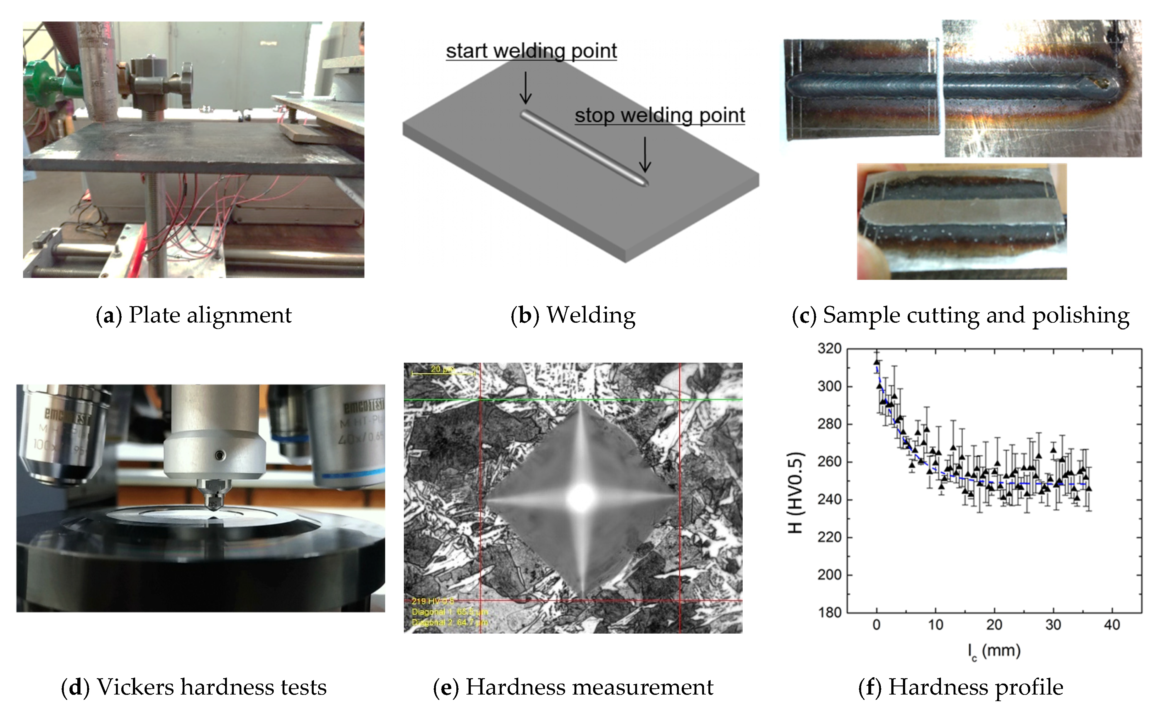
Aiming for a brief contextualization,
Figure 1 presents a summary of the experimental methodology adopted by Cruz Neto [
2], from the fixation and alignment of the specimens for the welding process to the adjustment of the AEF to the hardness profile, H versus l, for each specimen.
Table 1 presents the
,
,
,
,
,
and
values. The first column presents the identification of the specimen, with a total of 12. Each specimen is the result of a DOE testing, where the variables of process, consequently, in
Table 1, the values of
,
,
,
and
appear repeated for the same specimen, varying only the values of
and
(hardness profile). The
,
,
,
and
variables are candidates for level in multilevel modeling, since, in principle, hardness values could be nested, or grouped, according to any of these variables. Initially, specimen was used as a level and, although it was possible to adjust multilevel models, having specimen as a level represented little physically. Finally, we chose to use
as a level, since its value is associated with the heat flow in the material, having a physical relationship with the cooling rate and hardness values. The data set has a total of 871 observations, a small part of which is presented in
Table 1. To adjust the models, both the multilevel models and the ANN models, a randomly generated sample containing 70% of the observations was used, the remaining 30% was separated to evaluate and compare the different models obtained.
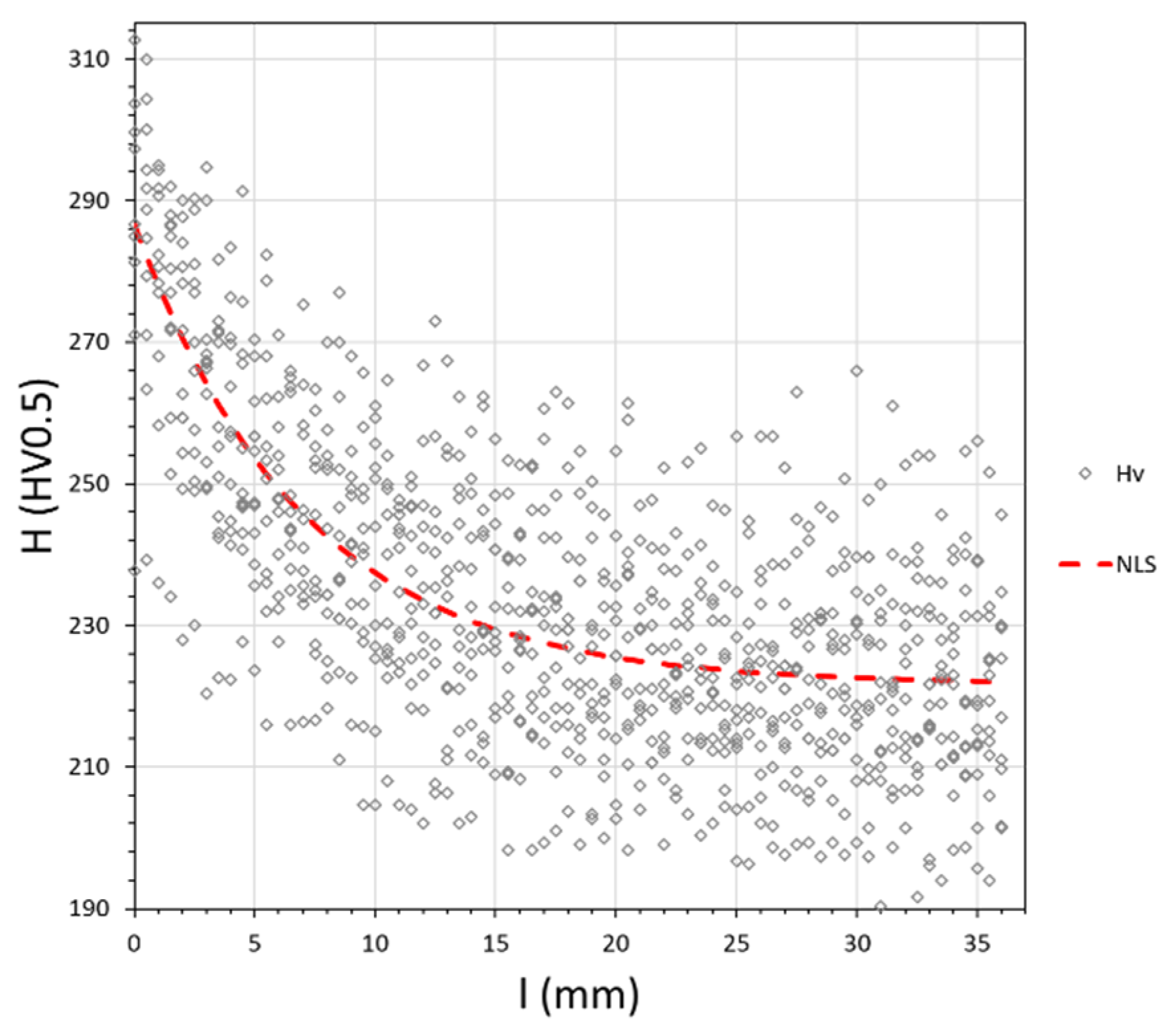
Before fitting the multilevel models, a single nonlinear regression model (NLS,
nonlinear squares) -
model_1 was fitted, as shown in
Figure 2, using the Gauss-Newton method, the standard method when using the package
“nls”.
model_1 will serve as a reference for evaluating the adjusted multilevel models later.
After fitting a single non-linear model, the applicability of multilevel modeling was investigated. To adjust the models, the package
“nlme” of the R language was used. First, a linear multilevel model was adjusted, using the function
lme, requiring the linearization of an asymptotic exponential model for this purpose, Equation (1).
where
is the length of the weld bead, it can be noted that for the linearization the
coefficient obtained in the adjustment of
model_1 was used. Therefore, we have the linearized multilevel model (LME,
linear mixed-effects) as shown in Equation (2):
where
and
are the LME coefficients and
the respective error terms, with observations
i nested in
j groups. It is worth nothing that, in this study, the observations will be grouped according to the values of
, as described in the previous section. The coefficients
and
represent the expected value of H for a given observation
i belonging to group
j, respectively, when
(general intercept) and where there is a unit change in the value of
,
ceteris paribus. And
e
represent the change in the expected value of
for a given observation
i belonging to group
j when there is unit variation, respectively, in the value of
and in the value of the product
,
ceteris paribus. In addition,
and
represent the error terms arising from the presence of observations from different groups in the dataset and indicate, respectively, the existence of randomness in the intercepts and the existence of randomness in the slopes of the models referring to the groups [
4]. Combining Equations (2.1)–(2.3), we arrive at Equation (3):
Rearranging the terms of Equation (3), the components of fixed effects and components of random effects are evident, as shown in Equation (4):
Analyzing Equation (4), if the statistical significance of the variances of the error terms
and
is not verified, that is, if both were statistically equal to zero, the model would be reduced to a multiple linear regression model, as shown in Equation (5):
In this scenario of the non-significance of the error terms
and
, Equation (5) could be estimated by traditional methods, such as Ordinary Least Squares (OLS). Therefore, we see the importance of running a test to determine whether the variance of the error terms
and
are significantly different from zero, and the results of these tests are presented in the next section.
Figure 3 shows how the LME named
model_2 was adjusted in the R script.
After adjusting the LME model, a nonlinear multilevel model (NLME
, nonlinear mixed-effects) was adjusted, called
model_3 in the R script, using the function
nlme, as shown in
Figure 4.
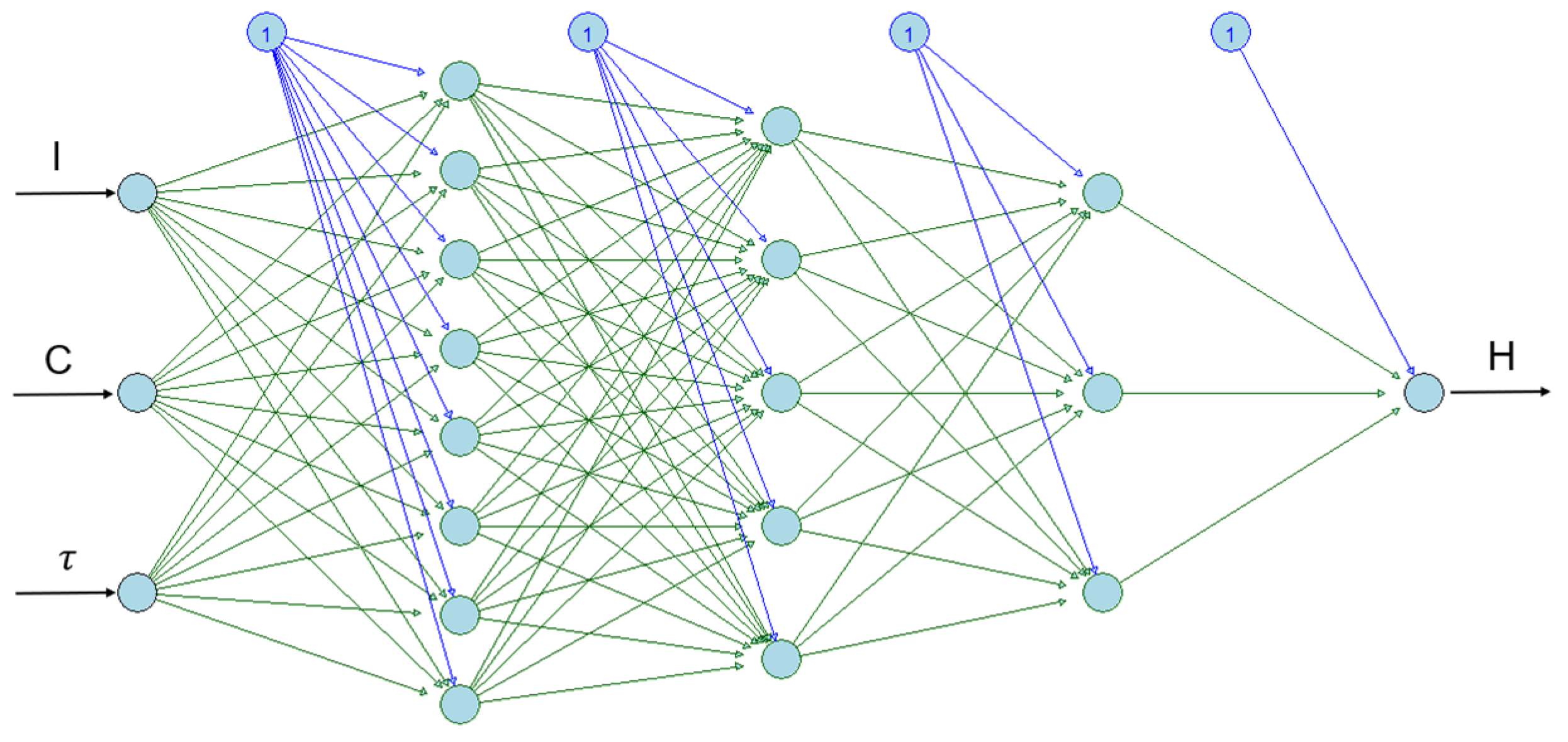
Finally, after obtaining the LME and NLME models, several ANN models were trained, always having as input neurons
,
and
and as output neuron the hardness of the weld bead
, as can be seen in
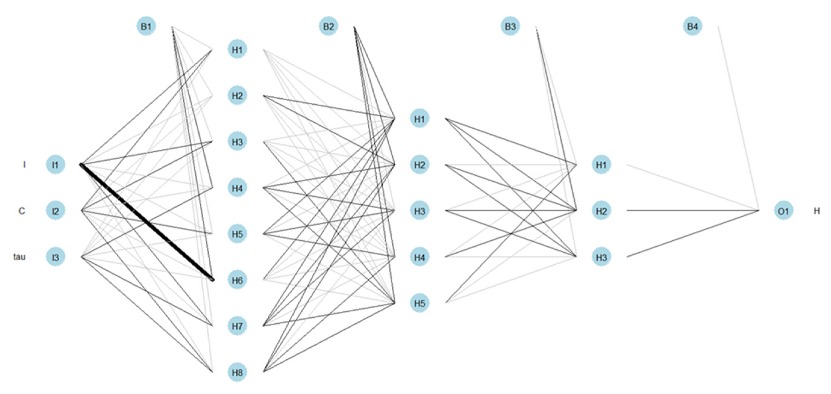
Figure 5 an architectural example. However, it is worth mentioning that several architectures were tested, modifying the number of neurons per hidden layer, number of hidden layers, type of activation function and the optimization method. For the training of the ANN, the packages
“neuralnet” and
“h2o” were used, and the commands in R language can be seen in
Figure 6.
4. Conclusions
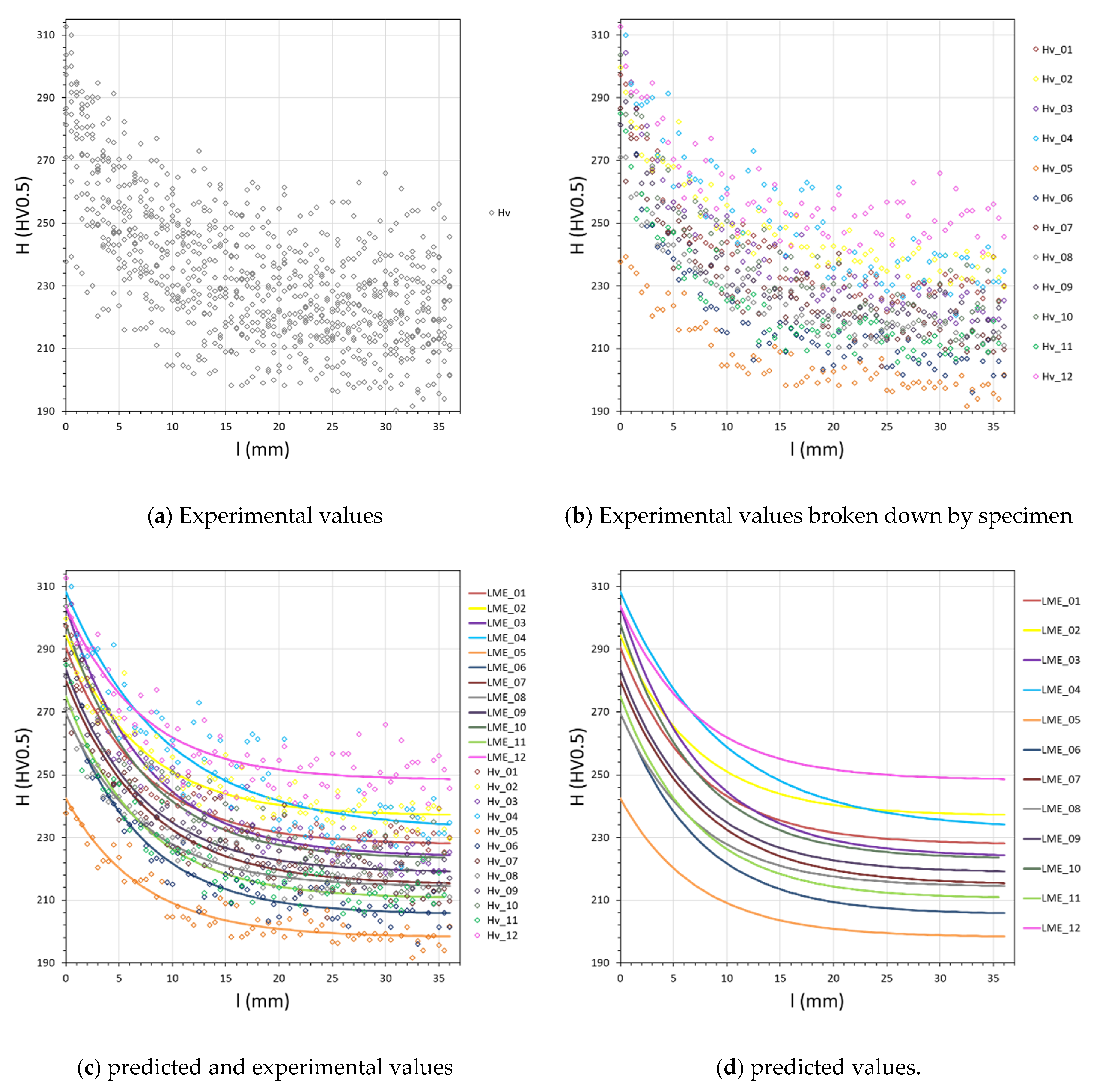
After testing the significance of the variance of the random terms of the LME model, the multilevel character of the data was verified. The existence of this hierarchical structure resulted in multilevel models, linear and non-linear, with predictive capacity superior to the single non-linear regression, NLS. After a few attempts, the choice of the variable as the level in the multilevel model was chosen. As a variable belonging to the level, success was achieved only by adding the variable as a predictor. Perhaps because the variables , and are already incorporated in the calculation of , their addition to the multilevel modeling did not add predictive capacity to the model. After evaluating the LME and NLME models, it was concluded that both models showed a good fit to the data, being considered equivalent by the metrics used. However, for the adjustment of the LME, it was necessary to linearize the exponential term, fixing the coefficient belonging to the argument of the exponential function, which is a limitation of this approach.
For the LME, the intraclass correlation revealed that is responsible for 48% of the variation along the weld bead . The influence of on the hardness values already been hypothesized. However, in a previous approach, performing several non-linear regressions, one for each group, it was not possible to isolate the influence of on the hardness values. Therefore, it is concluded that this explanatory capacity of the multilevel modeling is one of the greatest strengths of this methodology.
After several attempts, an ANN was obtained with a slightly better fit to the data than the multilevel models. However, since the multilevel models and the ANN models achieved equivalent evaluation metrics, the use of multilevel modeling is recommended, due to its greater explanatory capacity.
Figure 1.
Methodology used by Cruz Neto [
2]. (
a) Plate alignment; (
b) Welding; (
c) Sample cutting and polishing; (
d) Hardness profile; (
e) Hardness measurement; (
f) Vickers hardness tests.
Figure 1.
Methodology used by Cruz Neto [
2]. (
a) Plate alignment; (
b) Welding; (
c) Sample cutting and polishing; (
d) Hardness profile; (
e) Hardness measurement; (
f) Vickers hardness tests.
Figure 2.
R commands for non-linear model fitting with the package “nls”.
Figure 2.
R commands for non-linear model fitting with the package “nls”.
Figure 3.
R script to fit a linearized multilevel model with the function lme from the package “nlme”, using Restricted Estimation Maximum Likelihood (REML) as the coefficient fitting method.
Figure 3.
R script to fit a linearized multilevel model with the function lme from the package “nlme”, using Restricted Estimation Maximum Likelihood (REML) as the coefficient fitting method.
Figure 4.
R script to fit a non-linear multilevel model with the function nlme from the package “nlme”.
Figure 4.
R script to fit a non-linear multilevel model with the function nlme from the package “nlme”.
Figure 5.
Example architecture of an ANN model.
Figure 5.
Example architecture of an ANN model.
Figure 6.
R commands for ANN training, packages: (a) “neuralnet” and (b) “h2o”.
Figure 6.
R commands for ANN training, packages: (a) “neuralnet” and (b) “h2o”.
Figure 7.
Experimental hardness along weld bead and values predicted by non-linear regression model (NLS).
Figure 7.
Experimental hardness along weld bead and values predicted by non-linear regression model (NLS).
Figure 8.
Output of the function stderr_nlme, showing the significance test of the variance of the error terms and of the LME.
Figure 8.
Output of the function stderr_nlme, showing the significance test of the variance of the error terms and of the LME.
Figure 9.
Results obtained through the LME model – (a) Experimental values, (b) Experimental values broken down by specimen, (c) predicted and experimental values (d) predicted values.
Figure 9.
Results obtained through the LME model – (a) Experimental values, (b) Experimental values broken down by specimen, (c) predicted and experimental values (d) predicted values.
Figure 10.
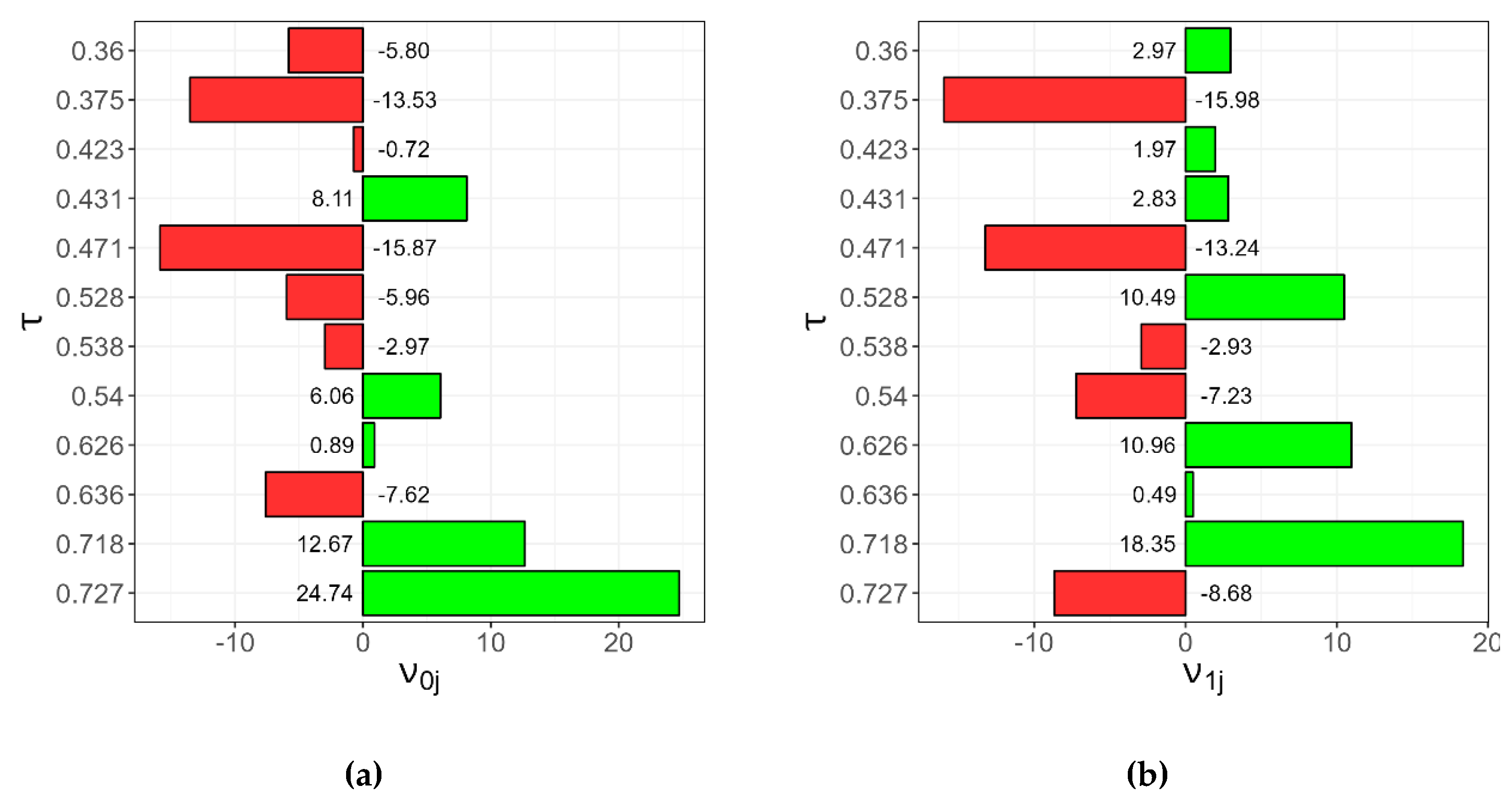
(a) Random intercept values and (b) random slopes of the LME model for each value of relative thickness .
Figure 10.
(a) Random intercept values and (b) random slopes of the LME model for each value of relative thickness .
Figure 11.
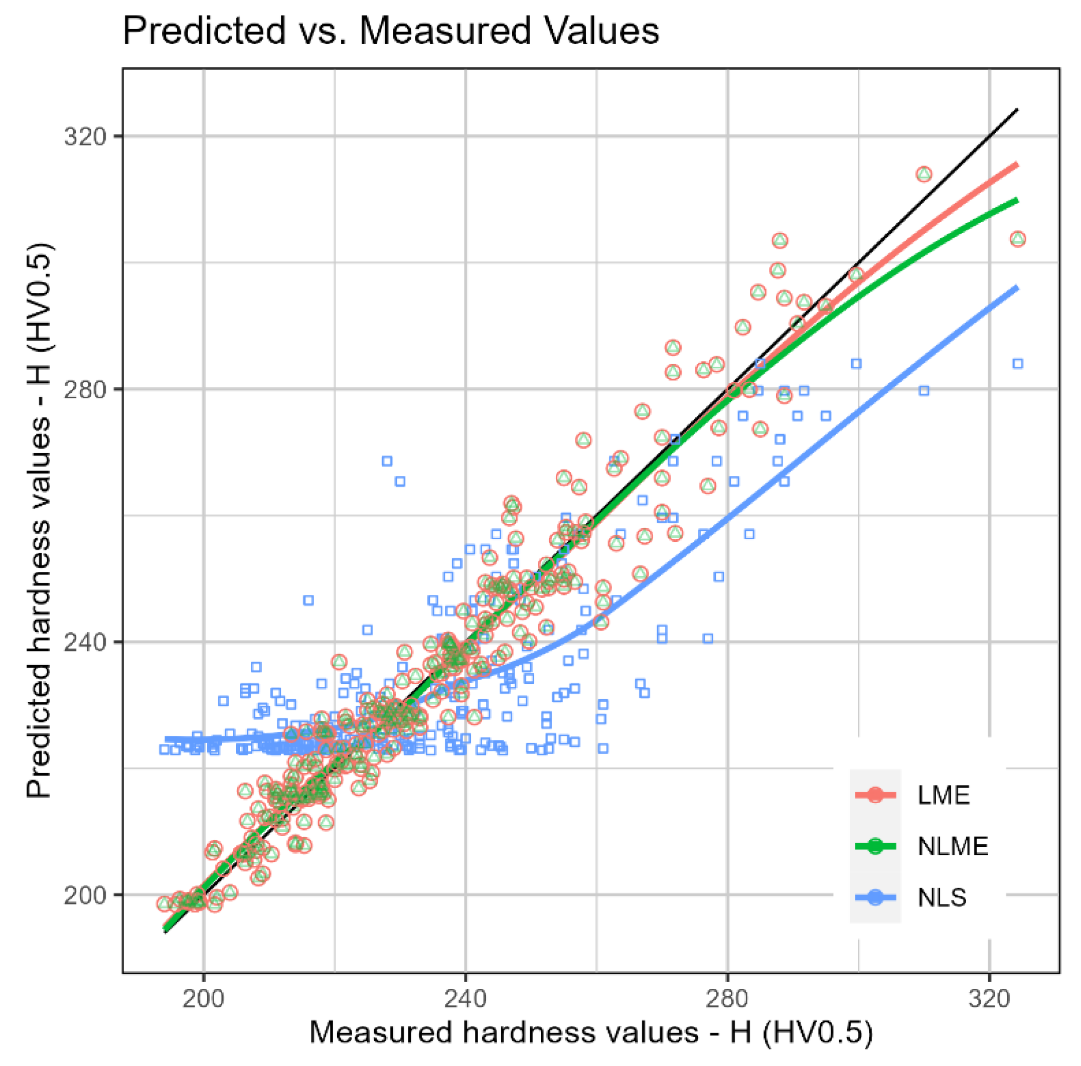
Experimental vs predicted values of H by the LME, NLME and NLS models.
Figure 11.
Experimental vs predicted values of H by the LME, NLME and NLS models.
Figure 12.
Output of the function lrtest of the package “lmtest”, showing the significance test of the difference between the LME and NLME models.
Figure 12.
Output of the function lrtest of the package “lmtest”, showing the significance test of the difference between the LME and NLME models.
Figure 13.
Architecture and representation of the weights of the ANN1 network.
Figure 13.
Architecture and representation of the weights of the ANN1 network.
Figure 14.
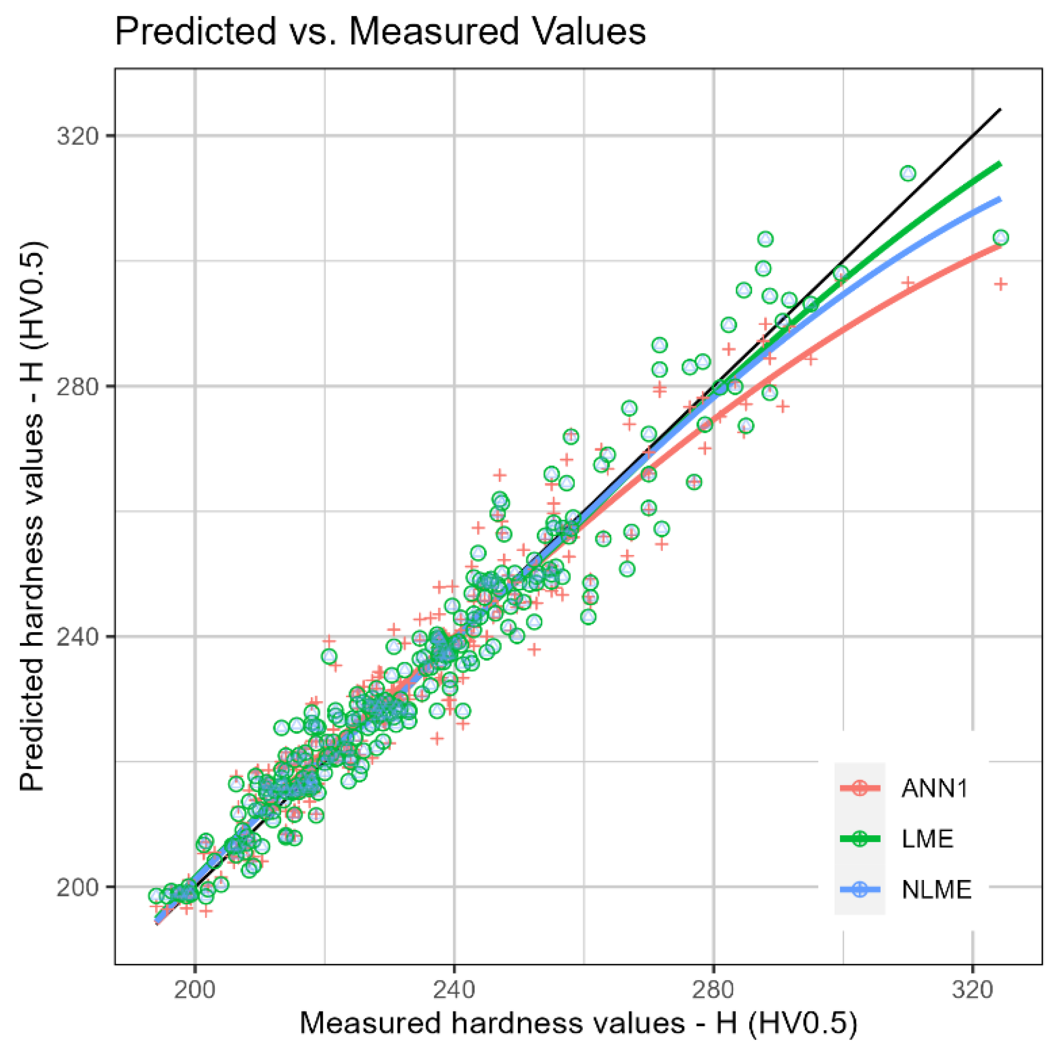
Experimental versus predicted values of H by the LME, NLME and ANN1 models.
Figure 14.
Experimental versus predicted values of H by the LME, NLME and ANN1 models.
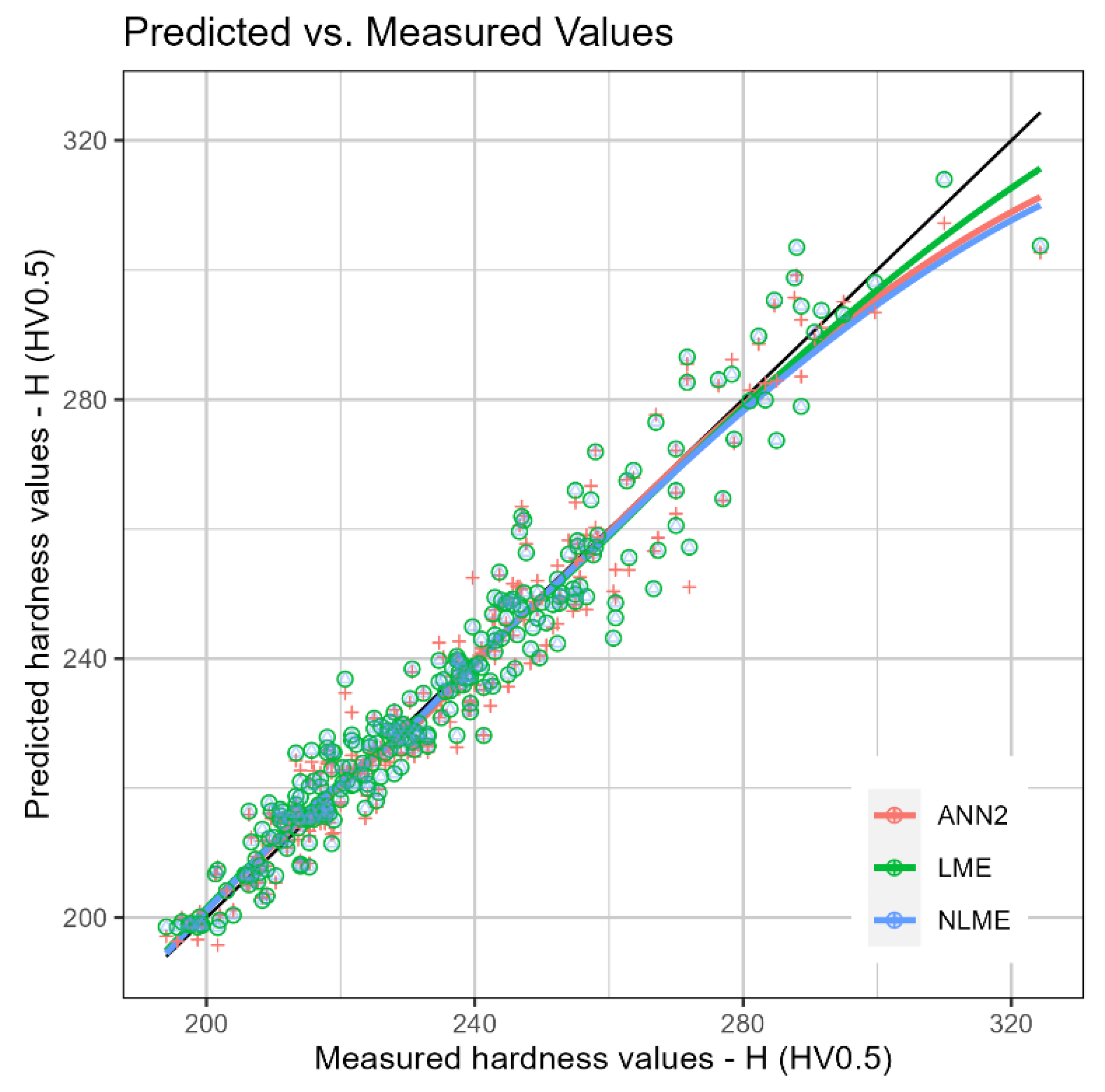
Figure 15.
Experimental versus predicted values of by the LME, NLME and ANN2 models
Figure 15.
Experimental versus predicted values of by the LME, NLME and ANN2 models
Table 1.
Data structuring for the adjustment of multilevel models.
Table 1.
Data structuring for the adjustment of multilevel models.
| SPECIMEN |
p (kW) |
v (mm/s) |
d (mm) |
C |
τ |
l (mm) |
H (HV0.5) 1
|
| 1 |
4.053 |
6.67 |
6.30 |
0.235 |
0.538 |
0.0 |
297.33 |
| 1 |
4.053 |
6.67 |
6.30 |
0.235 |
0.538 |
0.5 |
294.33 |
| 1 |
4.053 |
6.67 |
6.30 |
0.235 |
0.538 |
1.0 |
278.33 |
| 1 |
4.053 |
6.67 |
6.30 |
0.235 |
0.538 |
1.5 |
277.00 |
| • |
• |
• |
• |
• |
• |
• |
• |
| • |
• |
• |
• |
• |
• |
• |
• |
| • |
• |
• |
• |
• |
• |
• |
• |
| 1 |
4.053 |
6.67 |
6.30 |
0.235 |
0.538 |
34.5 |
231.33 |
| 1 |
4.053 |
6.67 |
6.30 |
0.235 |
0.538 |
35.0 |
239.33 |
| 1 |
4.053 |
6.67 |
6.30 |
0.235 |
0.538 |
35.5 |
225.33 |
| 1 |
4.053 |
6.67 |
6.30 |
0.235 |
0.538 |
36.0 |
230.00 |
| 2 |
3.114 |
5.00 |
6.30 |
0.235 |
0.540 |
0.0 |
299.67 |
| 2 |
3.114 |
5.00 |
6.30 |
0.235 |
0.540 |
0.5 |
291.67 |
| 2 |
3.114 |
5.00 |
6.30 |
0.235 |
0.540 |
1.0 |
282.33 |
| 2 |
3.114 |
5.00 |
6.30 |
0.235 |
0.540 |
1.5 |
280.33 |
| • |
• |
• |
• |
• |
• |
• |
• |
| • |
• |
• |
• |
• |
• |
• |
• |
| • |
• |
• |
• |
• |
• |
• |
• |
| 12 |
3.244 |
5.83 |
8.01 |
0.256 |
0.727 |
34.5 |
254.67 |
| 12 |
3.244 |
5.83 |
8.01 |
0.256 |
0.727 |
35.0 |
256.00 |
| 12 |
3.244 |
5.83 |
8.01 |
0.256 |
0.727 |
35.5 |
251.67 |
| 12 |
3.244 |
5.83 |
8.01 |
0.256 |
0.727 |
36.0 |
245.67 |
Table 2.
Metrics for evaluating the NLS, LME and NLME models.
Table 2.
Metrics for evaluating the NLS, LME and NLME models.
| |
NLS |
LME |
NLME |
| Log-likelihood |
-2544.04- |
-1951.27 |
-1964.09 |
| SSE |
63337.5 |
8590.1 |
8571.6 |
| MSE |
242.672 |
32.912 |
32.842 |
Table 3.
Metrics for evaluating the LME, NLME and ANN1 models.
Table 3.
Metrics for evaluating the LME, NLME and ANN1 models.
| |
LME |
NLME |
ANN1 |
| SSE |
8590.1 |
8571.6 |
1006.3 |
| MSE |
32.912 |
32.842 |
38.553 |
Table 4.
Metrics for evaluating the LME, NLME, ANN1 and ANN2 models.
Table 4.
Metrics for evaluating the LME, NLME, ANN1 and ANN2 models.
| |
LME |
NLME |
ANN1 |
ANN2 |
| SSE |
8590.1 |
8571.6 |
10062.3 |
8415.6 |
| MSE |
32.912 |
32.842 |
38.553 |
32.244 |
