Preprint
Article

Physics-Informed Neural Network for Solving a 1-Dimensional Solid Mechanics Problem

Altmetrics

Downloads

151

Views

71

Comments

0

A peer-reviewed article of this preprint also exists.

Submitted:

23 September 2024

Posted:

24 September 2024

You are already at the latest version

Alerts
Abstract
Our objective in this work is to demonstrate how Physics-Informed Neural Networks, a type of deep learning technology, can be utilized to examine the mechanical properties of a helicopter blade. The blade is regarded as a prismatic cantilever beam that is exposed to triangular loading, and comprehending its mechanical behavior is of utmost importance in the aerospace field. PINNs utilize the physical information, including differential equations and boundary conditions, within the loss function of the neural network to approximate the solution. Our approach determines the overall loss by aggregating the losses from the differential equation, boundary conditions, and data. We employed a Physics-Informed Neural Network (PINN) and an Artificial Neural Network (ANN) with equivalent hyperparameters to solve a fourth-order differential equation. By comparing the performance of the PINN model against the analytical solution of the equation and the results obtained from the ANN model, we have conclusively shown that the PINN model exhibits superior accuracy, robustness, and computational efficiency when addressing high-order differential equations that govern physics-based problems. In conclusion, the study demonstrates that PINN offers a superior alternative for addressing solid mechanics problems with applications in the aerospace industry.
Keywords: 
Subject: Computer Science and Mathematics  -   Artificial Intelligence and Machine Learning

1. Introduction

Solid mechanics can be described as a field within applied mechanics concerned with analyzing how solid objects respond to different types of forces. It explores how materials behave under various loading conditions, offering insights into their structural integrity and performance [1]. Mechanical problems are represented using a variety of differential equations, which take different forms depending on the nature of the problem.
In recent years, computational solid mechanics has emerged as a discipline that uses numerical techniques to solve complex differential equations [2]. Solving these problems analytically is challenging and time-consuming because of the intricate equations and irregular problem domains. Over the years, various numerical techniques have been developed, such as the finite element method (FEM) [3], finite difference method (FDM) [4], element-free Galerkin method [5], and mesh-free methods [6]. Among these methods, FEM is the most widely used numerical method to solve problems in the area of solid mechanics. In numerous cases, the problem to be solved is extensive, resulting in simulation time ranging from hours to days or even weeks. This incurs a high computational cost. If there is a requirement to change the parameter, the complete analysis must be done again from scratch, which is quite time-consuming [7,8].
Over the past few years, Artificial neural networks (ANNs) have demonstrated remarkable performance in various fields such as image classification [9], time series forecasting [10], predictive analytics [11], genomics [12] and natural language processing [13], owing to their capacity to grasp intricate patterns and relationships from data. Artificial neural networks (ANNs) can incorporate multiple hidden layers containing neurons, granting them robust learning capabilities. This feature enables ANNs to offer an alternative method for addressing mechanics problems, diverging from conventional numerical solvers. Artificial neural networks (ANNs) have proven effective in addressing a range of challenges in fluid mechanics [14,15], fracture mechanics [16], and solid mechanics [17]. Nonetheless, their performance tends to be strongest when abundant data is available. In mechanics problems, data can be scarce, and ANNs do not incorporate the underlying physical laws of the engineering problem, resulting in reduced prediction accuracy [8,18]. So, the challenges associated with artificial neural networks (ANNs) motivate us to explore new ideas and methods.
One such approach widely accepted in the scientific community is a deep learning-based method known as Physics-Informed Neural Networks (PINNs) introduced by Raissi et al. [19]. PINNs represent a highly effective method for addressing problems governed by partial differential equations (PDEs). These networks are designed to directly integrate physical laws or constraints into their structure, enabling them to simulate and accurately model complex systems. The foundational component of the Physics-Informed Neural Network (PINN) framework is a Multi-Layer Artificial Neural Network that is enhanced with a physics-informed loss function. This innovative loss function integrates governing differential equations, boundary conditions, initial conditions, and any available data to determine the total loss accurately. The sole distinction between an Artificial Neural Network (ANN) and a Physics-Informed Neural Network (PINN) lies in how the loss function is implemented and calculated [20]. Artificial neural networks (ANNs) rely solely on data for learning, whereas Physics-Informed Neural Networks (PINNs) incorporate the governing equations as pre-existing knowledge [21]. PINNs can be effective in scenarios where labeled data is sparse because they utilize both the existing data as well as the inherent physical principles described in equations. Compared to ANNs, PINNs require less data. PINNs differ from traditional numerical methods like the Finite Difference method and finite element because they are not mesh-based. Instead, they are a mesh-free method, which allows them to handle irregular and complex geometries [19,22].
In their seminal work, Raissi et al. [19] tackled two distinct problem sets: data-driven solution and data-driven discovery within the realm of partial differential equations. Under the data-driven solution framework, they addressed the Schrodinger Equation and the Allen-Cahn equation. Meanwhile, within the data-driven discovery approach, they delved into the Navier-Stokes Equation and the Korteweg–de Vries equation. After their introduction, PINNs are used in solving various other PDEs [23,24,25]. PINNs can be used for solving supervised learning problems [26] as well as unsupervised learning tasks [27]. They can also be employed for both forward and inverse problems [28]. Due to their ability to incorporate the governing equations of the problems, PINNs are used in various fields such as fluid mechanics [29], heat transfer [30], healthcare [31], finance [32] and solid mechanics [33]. Several research studies have been carried out on implementing PINNs so far. In one of the studies, Haghighat et al.(2021) [33] created a PINN structure to anticipate the field variables (such as displacement and stress) associated with linear elastic and non-linear problems. In their study, Rao et al.(2021) [34] applied enforced initial and boundary conditions to simulate static and dynamic problems using a PINN model, which gives mixed-variable output. One of the works done by J.Bai et al.(2022) [35] proposed the LSWR loss function for PINNs, which uses the Least Squares Weighted Residual (LSWR) method, solved 2D and 3D solid mechanics problem and showed that the performance of PINN based on LSWR loss function is much effective and accurate compared to PINNs utilizing either Collocation or energy-based loss functions. In the study by J.bai et al.(2023), [36], the focus was on programming methods in executing governing equations. They solved the 1, 2, and 3 dimensions problems by employing collocation-based and energy-based loss functions, demonstrating the effectiveness of PINN-based Computational Solid Mechanics. Abueidda et al.(2022) [37] applied PINNs to solve 3-dimensional Hyperelastic problems. The work by Kapoor et al.(2023) [38] used PINNs to simulate complex beam systems, solving both forward and inverse problems. Also, Verma et al. (2024) [39] use PINNs to simulate the behavior of a cantilever beam subjected to a uniform loading. There is a resonable amount of work that shows PINNs are effective in solving PDEs.
In our study, we analyze the mechanical characteristics(such as deflection, etc.) of a helicopter blade treated as a prismatic(constant E I ) cantilever beam subjected to triangular loading. When a lateral force is applied over a beam, the beam’s longitudinal axis undergoes deformation, resulting in a curvature known as the deflection curve [1]. Understanding these mechanical behaviors is essential in designing helicopter blades, ensuring optimal flight performance and safety. This research is dedicated to investigating the capabilities of Physics-Informed Neural Networks (PINNs) within beam mechanics, emphasizing their applicability and significance in aerospace design and analysis.
The paper is organized as follows: Section 2 thoroughly explains the theory and architecture of ANNs and PINNs. Section 3 gives a brief overview of the problem to be solved and defines the governing equation, boundary conditions, and the formulation of the loss function for PINN. Section 4 presents a detailed exploration of the training process and a brief overview of the results obtained. Ultimately, the study is concluded in Section 5.

2. Physics-Informed Neural Network

This section provides a detailed exploration of artificial neural networks (ANNs) and physics-informed neural networks (PINNs), focusing on their theoretical frameworks and methodologies and how they are used to address challenges in computational solid mechanics.

2.1. Artificial Neural Network

Inspired by the biological neurons present in the human brain [40], the artificial neural network is a computational model that aims to replicate the functions of neurons, allowing them to learn patterns and relationships from the data inputs and make a decision or prediction based on the acquired knowledge [41].
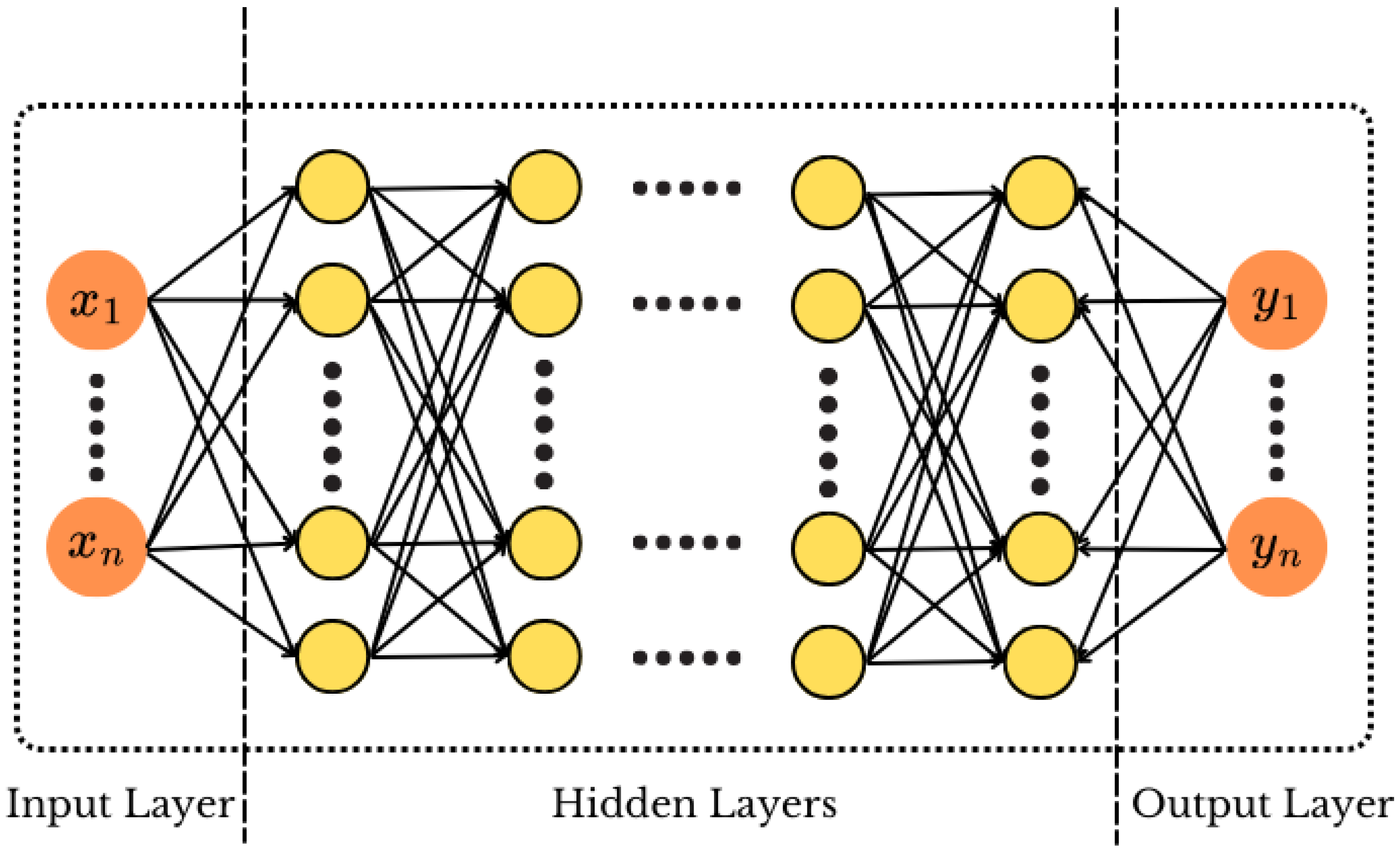
The artificial neural network (ANN) architecture, illustrated in Figure 1, comprises several network layers, including an input layer, hidden layer(s), and an output layer. Depending on the requirements of the problem, each neural network layer can contain multiple neurons or nodes. Data or information is inputted into the neural network via the input layer and then moves forward through the network, passing through the adjacent layers, which are connected to each other via weights, biases, and activation functions [21]. Typically, an L-layer artificial neural network can be mathematically expressed as [36,42]:
ϕ ( 0 ) = x ,
ϕ ( l ) = w ( l ) · ϕ ( l 1 ) + b ( l ) , for l = 1 , 2 , , L 1 ,
ϕ ( l + 1 ) = α ( ϕ ( l ) ) ,
v = ϕ ( L ) = w ( L 1 ) · ϕ ( L 1 ) + b ( L 1 ) .
where x is the input vector which is fed into the input layer ϕ ( 0 ) = x , adjacent layers in the neural network are denoted as ϕ ( l ) and ϕ ( l + 1 ) . The activation function is represented by α , and the final output of the artificial neural network (ANN) is denoted by v.
Figure 1. Artificial Neural Network architecture
Preprints 119088 g001
A neural network tries to establish a relationship between the input data ( x ) and output data ( y ) by learning an underlying function ( f ) . This relationship is defined by a function v = f ( x , θ ) , where θ refers to the learnable parameters of the network [43]. The network works to optimize these parameters by reducing a loss function:
L NN = 1 N i = 1 N v v * 2
where N is the number of data points; it measures the difference between the network’s predictions v and the actual values v * . The neural network can effectively model the desired function by adjusting its parameters during the training process. Finally, the prediction or result is delivered through the output layer.

2.2. Physics-Informed Neural Networks(PINNs)

Physics-Informed Neural Networks (PINNs), as proposed by Raissi et al. [19], offer a novel approach to solving problems governed by Partial Differential Equations (PDEs). This technique seamlessly integrates the core principles and equations of physics into the training process of artificial neural networks (ANNs).
The general representation of a governing equation for a physical process is given by [8]:
u t = D ( u ) + P ( u ) ,
Here, D denotes the nonlinear differential operator, P represents the linear differential operator, and u stands for the unknown solution being analyzed, which satisfies the differential equation. The differential equation loss, L DE is as follows:
L DE = 1 N DE i = 1 N DE u ( x n , t n ) t D u ( x n , t n ) P u ( x n , t n ) 2 ,
where ( x n , t n ) denotes the collocation points where differential equation loss is calculated and N DE gives the total number of these collocation points. Also, the boundary and initial condition loss is given as:
L BC = 1 N BC i = 1 N BC B ( u ( x b , t b ) ) 2
L in = 1 N in i = 1 N in ( u ( x i , 0 ) u i ( x i , 0 ) ) 2
where ( x b , t b ) are the boundary points, N BC are the total number of boundary points, B is the boundary operator corresponding to Dritchlet, Robin, periodic or Neumann boundary conditions [44]. Also, ( x i , 0 ) are the initial points where initial loss is calculated, N are the total number of initial points, and u i is the defined initial condition for the problem. Also, the data loss is defined as:
L data = 1 N data i = 1 N data u ( x d , t d ) u es ( x d , t d ) 2
where ( x d , t d ) are the data points for training the ANN, N data are the total number of these data point, u es is the exact solution of the problem.
In the PINN approach, the aim is to effectively approximate the solution u of a given problem using a neural network. To achieve this, the network optimizes its parameters, which include weights and biases, by minimizing a defined loss function. This loss function is designed to ensure that the network accurately represents the underlying physics of the problem while also fitting the available data. In this study, our focus is solely on the differential equation loss ( L DE ), boundary loss ( L BC ), and data loss ( L data ). Therefore, the total loss is defined as follows:
L total = L DE + L BC + L Data ,
The architecture utilized in this study, as illustrated in Figure 2, centers around the Artificial Neural Network (ANN) as its primary component. This ANN comprises interconnected layers of artificial neurons, responsible for processing input data denoted as x and propagating information throughout the network to generate an output prediction, denoted as u. Subsequently, the output u is employed to compute derivative terms, which are obtained analytically through automatic differentiation methods [45]. These derivatives are then utilized to calculate the boundary and differential equation loss. The data loss is also directly computed based on the output u. Finally, the total loss, which requires minimization for practical training, is determined by considering all these factors.
Figure 2. Physics-infromed Neural Network architecture
Preprints 119088 g002

3. PINN for 1D Solid Mechanics Problem

In this section, we will discuss the problem that Physics-Informed Neural Networks (PINNs) aim to solve. We will explain the differential and exact equations, as well as the boundary conditions that govern the problem. Furthermore, we elaborate on the formulation of the loss function integrated into PINNs for addressing this particular problem.

3.1. Problem Definition

In this demonstration, we present the implementation of a Physics-informed Neural Network designed for solving a beam mechanics problem. We considered the helicopter blade as a cantilever beam which is fixed at point A and B is the free end, subjected to triangular loading, as illustrated in Figure 3.
The load intensity along the beam’s length L is defined by the equation:
q = q o ( L x ) L ,
Here, q o represents the maximum load applied at the fixed end, L denotes the length of the beam, and x signifies the position along the beam’s length.

3.2. Governing Equations

For a prismatic cantilever beam, the governing fourth-order differential equation according to Euler-Bernoulli theory is given by [1]:
E I d 4 v d x 4 = q ,
E I d 4 v d x 4 = q o ( L x ) L ,
Here, E represents Young’s Modulus, I denotes the Moment of Inertia of the beam, and q stands for the load intensity.
Upon integrating Equation (14) once, we obtain the expression for shear force (V) within the beam:
V = E I d 3 v d x 3 = q o ( L x ) 2 2 L + C 1 ,
and as we know, at the free end of the beam, i.e., at point B where x = L shear force is zero, so from this condition we have the following boundary condition
d 3 v d x 3 x = L = 0 ,
By using this condition and using Equation (15), we get C 1 = 0. Therefore, the shear force is given by,
V = E I d 3 v d x 3 = q o ( L x ) 2 2 L ,
Integrating Equation (14) twice yields the subsequent equation for the bending moment, M of the beam:
E I d 2 v d x 2 = q o ( L x ) 3 6 L + C 2 ,
At the free end, located at x=L, the bending moment is zero. This condition translates into the boundary condition:
d 2 v d x 2 x = L = 0 ,
By using the above boundary condition and the Equation (17), we get C 2 = 0, therefore the bending moment, M is
M = E I d 2 v d x 2 = q o ( L x ) 3 6 L ,
Continuing with the integration of Equation (14) for the third time, we derive the equation representing the slope.
E I d v d x = q o ( L x ) 4 24 L + C 3 ,
and at the fixed support slope is zero, so
d v d x x = 0 = 0 ,
which gives us
C 3 = q o L 3 24 ,
After substituting the value of C 3 into Equation (20) and simplifying, we obtain the equation defining the slope as follows:
d v d x = q o x 24 L E I ( 4 L 3 6 L 2 x + 4 L x 2 x 3 ) ,
Integrating Equation (14) four times yields the equation for deflection, which can be expressed as follows:
E I v = q o ( L x ) 5 120 L + C 3 x + C 4 ,
Here, we know the value of C 3 . Also, at the fixed support deflection of the beam is zero, which gives the following boundary condition:
v x = 0 = 0 ,
By using the above boundary condition, we get the value of,
C 4 = q o L 4 120 ,
Upon substituting the values of C 3 and C 4 and performing some simplifications, we obtain the exact equation that describes the deflection of the beam.
v = q o x 2 120 L E I ( 10 L 3 10 L 2 x + 5 L x 2 x 3 ) ,

3.3. Loss-Defined

In the preceding section, we derived the governing differential equation and the boundary conditions, laying the foundation for constructing the loss function for the Physics-informed Neural Network. The governing differential equation and boundary conditions are as follows:
E I d 4 v d x 4 = q o ( L x ) L ,
v ( 0 ) = 0 ,
v ( 0 ) = 0 ,
v ( L ) = 0 ,
v ( L ) = 0 ,
PINN is trained to approximate the solution to the differential equation over the boundary and collocation points, denoted as:
v PINN v ,
Using these equations(Equation (28) to Equation (32)), we formulate our boundary loss and physics-based loss, which enable learning of the neural network parameters by minimizing the total loss defined as [20]:
L total = L DE + L BC + L Data ,
where, L DE represents the differential equation loss:
L DE = 1 N DE i = 1 N DE | E I d 4 v PINN ( x n ) d x 4 + q o ( L x ) L | 2 ,
In this expression, x n denotes collocation points along the length of the beam for which L DE is calculated, and N DE represents the total number of collocation points.
As for the Boundary loss L BC it can be expressed as:
L BC = 1 N BC i = 1 N BC , ( L B 1 + L B 2 + L B 3 + L B 4 ) ,
L B 1 = | v PINN ( x b = 0 ) 0 | 2 ,
L B 2 = | v PINN ( x b = 0 ) 0 | 2 ,
L B 3 = | v PINN ( x b = L ) 0 | 2 ,
L B 4 = | v PINN ( x b = L ) 0 | 2 ,
here x b denotes the boundary points and N BC denotes the number of boundary points for the beam. L B 1 , L B 2 , L B 3 and L B 4 correspond to the boundary conditions defined in equations Equation (30) to Equation (32), with L representing the length of the beam.
The data loss, L Data , measures the deviation or difference between predicted values from the exact values and is defined as:
L Data = 1 N Data i = 1 N Data | v PINN ( x n ) v * ( x n ) | 2 ,
here N Data is the total number of collocation points on the beam used for calculating data loss, x n denotes the collocation points along the length of the beam, and v PINN is the predicted or approximated solution and v * is the exact solution.
So, to train the PINN model and learn the neural network parameters, the total loss( L total ) is minimized as much as possible. By minimizing this total loss, we fine-tune the model to make more accurate predictions, essentially improving its performance.

4. Results and Discussion

We considered a 1D cantilever beam of length, L=1m, subjected to a maximum load at point A, q 0 = 1 . 0 N as shown in Figure 3. For the simplification of the problem, we assume the value of Young’s modulus, E = 1 . 0 P a , and Moment of Inertia, I = 1 . 0 K g m 2 .
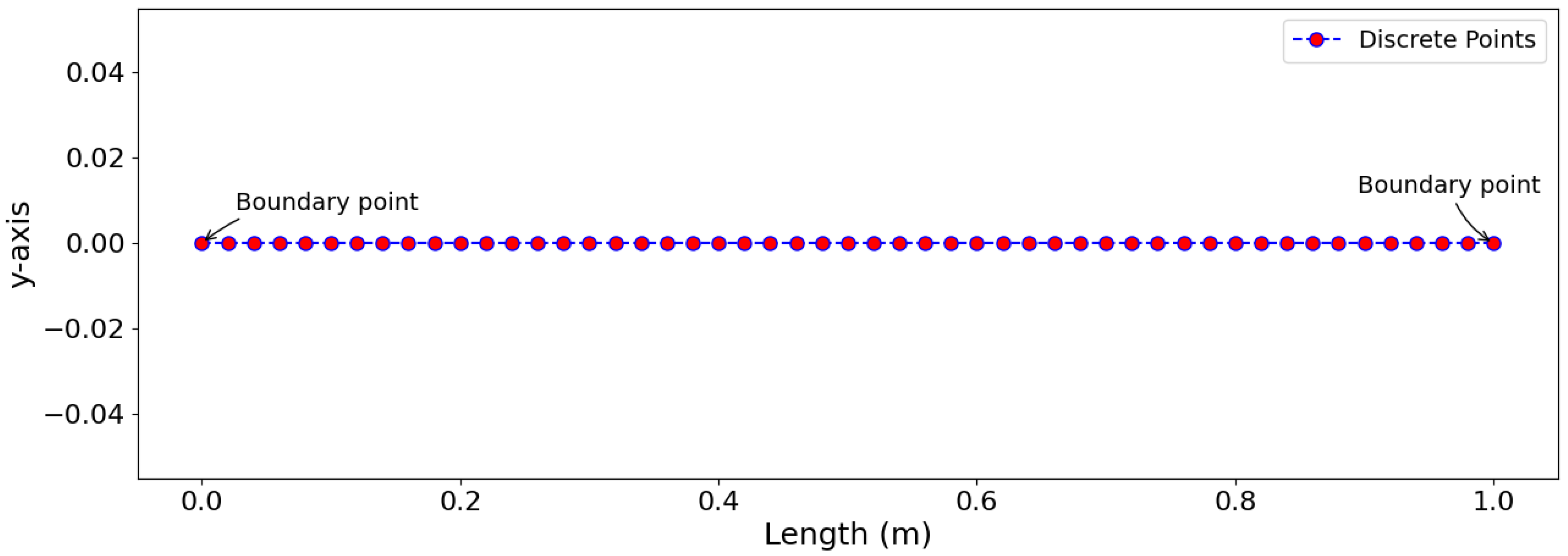
In this study, we analyzed 51 collocation points spaced at intervals of 0.02 meters along the length of the beam as shown in Figure 4. At the boundary points, we selected two positions: one at the fixed end ( x = 0 ) and another at the free end ( x = L ) as shown in Figure 4. Thus, we have N De = N data = 51 and N BC = 2 , with collocation points x n ranging from 0 to 1 with increments of 0.02 and the boundary points x b ϵ [ 0 . 00 , 1 . 00 ] .
We trained the PINN model for 300 epochs at a learning rate of α = 0 . 001 , employing ADAM [46] as the optimizer. The model consists of an architecture with 1 input layer, 5 hidden layers, and 1 output layer, each hidden layer containing 50 neurons. For the activation function, we implemented the tanh function [47] as shown in Equation (42).
T a n h ( x ) = e x e x e x + e x ,
We also trained an Artificial Neural Network (ANN) with an identical network architecture for comparison purposes. This includes the same number of epochs, learning rate, optimizer and the tanh activation function, allowing for a direct comparison between the PINN model and the ANN. Both the models were developed from scratch using PyTorch [48] version 2.2.1. We have summarized all the details of our models in Table 1.
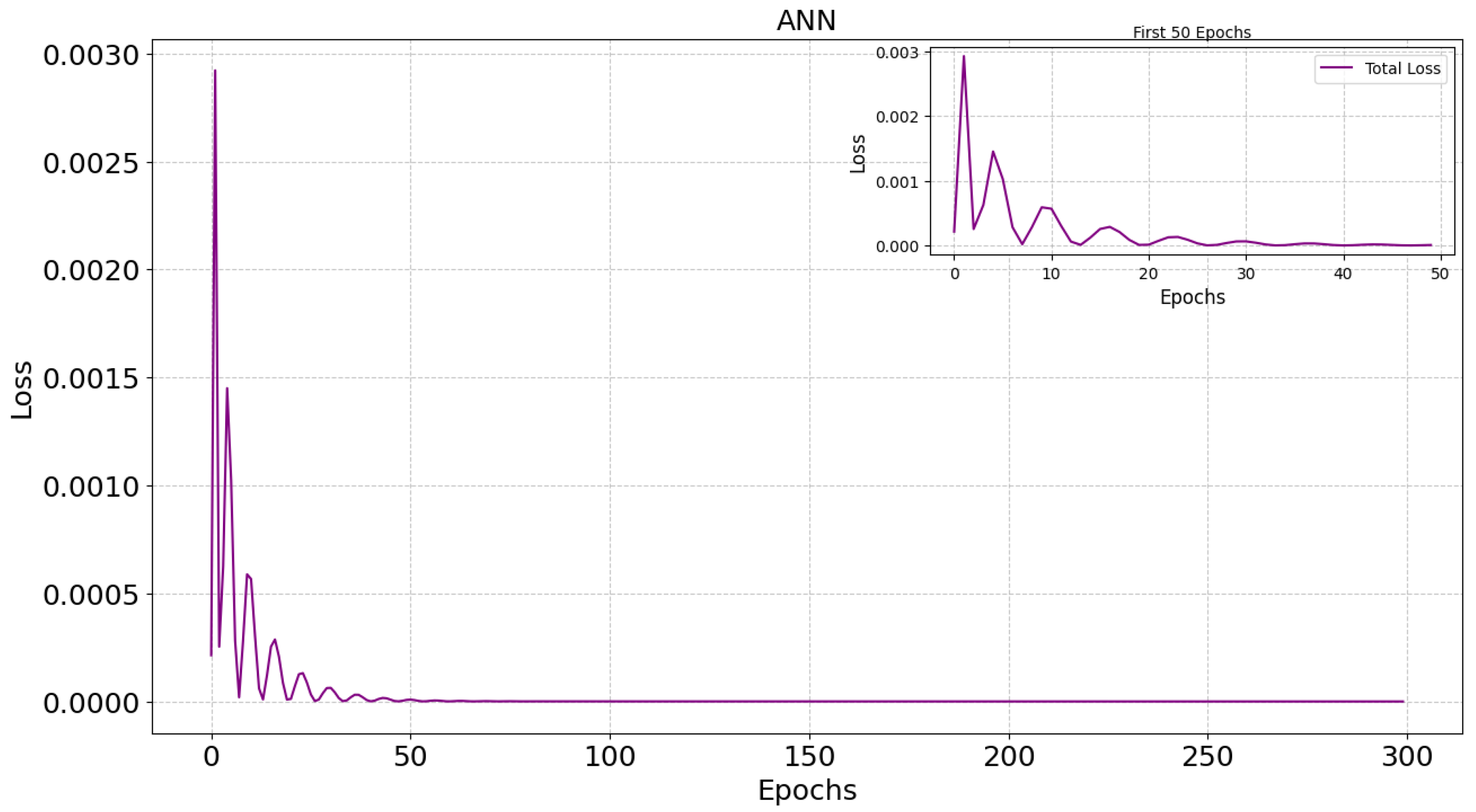
The ANN model underwent training using the configuration outlined in Table 1. Upon completion of 300 epochs of training, a loss curve for the model was generated, visually represented in Figure 1. This curve serves as a valuable tool for assessing the model’s convergence and performance throughout the training process.
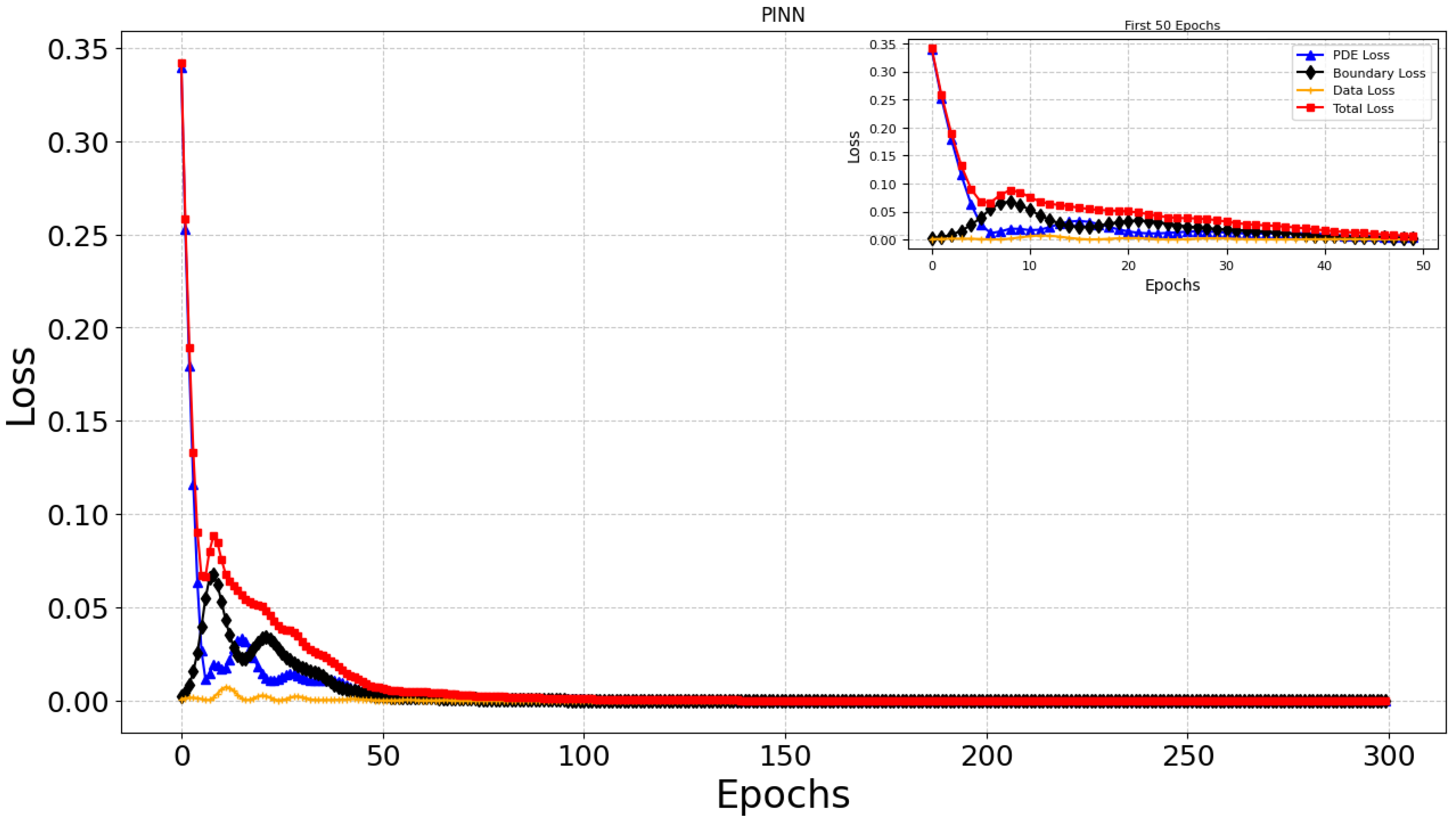
Also, after training the PINN model for 300 epochs, we acquired the loss curve, depicted in Figure 5. This graph illustrates the convergence of various components, including PDE loss, Boundary loss, data loss, and the overall Total Loss.
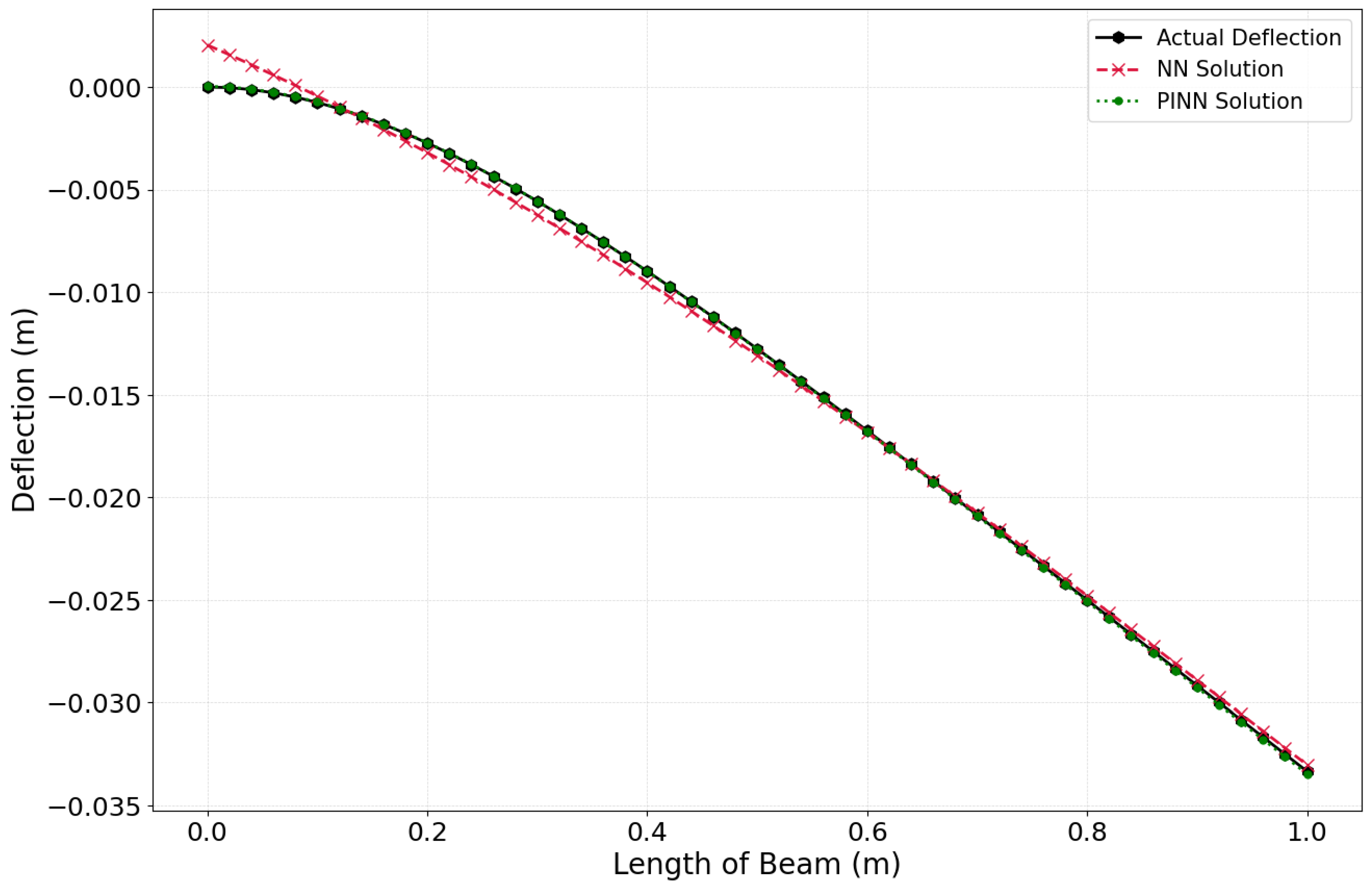
Upon completing its training, the PINN model can accurately predict/approximate the deflection, slope, bending moment, and shear force along the length of a beam as shown in Figure 6 and Figure 7. This detailed analysis enables a precise evaluation of the beam’s mechanical response.
Also, we have calculated the Mean Squared Error (MSE) values between the predicted and the exact solution for both the models as shown in the Table 2. It is calculated as the average of the squared as errors as shown in equation Equation (43). It serves as a metric to evaluate the precision of a predictive model.
MSE = 1 n i = 1 n ( y ^ i y i ) 2
where n is the number of data points, y ^ i is the predicted value and y i is the actual/exact solution. A lower MSE value signifies enhanced performance, denoting that the predictions generated by the model are in closer approximation to the exact values.
As observed from Table 2, it is evident that the PINN model exhibits superior performance in approximating the solution of the differential equation when compared to the ANN model. Now, we delve into the outcomes achieved, presenting a comparative analysis of the results derived from PINN and ANN. This comparison is visually represented in Figure 6 and Figure 7.
As illustrated in Figure 6, the deflection curve predicted by the PINN overlaps with the exact deflection curve(obtained from the exact deflection equation, Equation (27)), demonstrating a high degree of accuracy. Conversely, the deflection curve derived from the ANN exhibits a noticeable deviation from the exact solution. In our method, we are giving the data points (i.e., collocation points generated along the length of the beam) as input to the neural network in both models, which tries to map a function between the data points and the deflection over the beam, but the difference arises in the implementation of the loss function. In PINNs, we include scientific or physical principles with the fitting of available data within the loss function framework, thereby ensuring a more holistic model. Conversely, in ANN, the loss function’s formulation is exclusively based on empirical data without integrating physical laws or constraints. The differential equation for deflection(Equation (14)) of the cantilever beam is of the fourth order, which we are approximating through PINNs and ANN. Additionally, the loss curve for both models, as depicted in Figure 5 and Figure 8, demonstrates good convergence. However, the complex nature of the governing equation, with its high order and non-linearity, poses challenges for the ANN model in accurately approximating the solution. As a result, the model exhibits a deviation from the exact deflection curve.
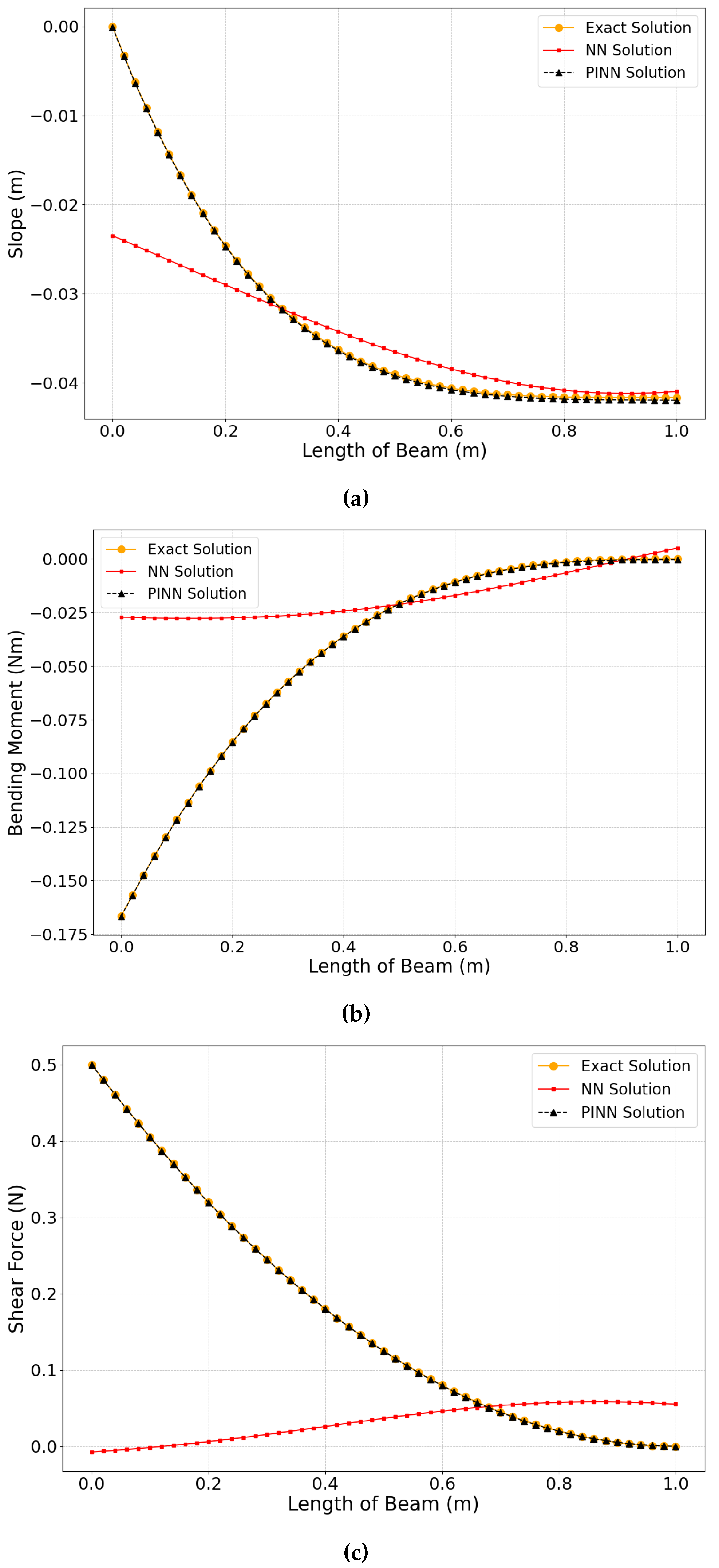
Additionally, we have also predicted the slope, bending moment, and shear force experienced by the beam along its length under triangular loading. The comparative analysis among the curves representing the exact solution, PINN solution, and the solution obtained through ANN is illustrated in Figure 7. As observed in Figure 7, the solution derived from the PINN perfectly matches the exact solution. Conversely, the solution obtained through ANN exhibits significant deviations. The calculation of slope, bending moment, and shear force is achieved through the differentiation of the output provided by the neural network in both models.
The slope is calculated as the first derivative of the deflection equation (Equation (27)). In Figure 7a, the PINN solution aligns with the exact solution, while the ANN solution does not achieve this level of accuracy. We aim to establish a function that maps the data points to the deflection of the curve using both PINN and ANN models. The output from the neural networks of both models is differentiated for the first time to determine the slope of the cantilever beam. But the result from the PINN model is significantly better than the ANN models.
The bending moment of the cantilever beam is determined by taking the second derivative of the deflection equation (Equation (27)). The comparison in Figure 7b shows that the PINN solution closely aligns with the exact solution, while the ANN solution does not. Here, the output from the neural network of both models is differentiated two times to get the bending moment of the cantilever beam under triangular loading. But, the PINN solution demonstrates superior performance compared to the ANN solution.
By taking the third derivative of the bending equation (Equation (27)), we can determine the shear force in the cantilever beam under triangular loading. As shown in Figure 7c, the PINN solution closely matches the exact solution, while the predicted solution by the ANN does not. Here also, the output from the neural network of both models is differentiated three times, which gives us the shear force. Once again, the predicted solution from the PINN model outperforms the ANN solution.
From the above results in predicting deflection, slope, bending moment and shear force it is clear that the PINN apporoch performs much better as compared to the ANNs because PINNs incorporate physical constraints into their loss function, giving them an advantage over conventional ANNs. Unlike PINNs, ANNs depend exclusively on the dataset provided and thus encounter challenges in accurately predicting the solution.
The predicted solution given by the ANN model, in comparison to the deflection curve(Figure 6), deviated less as compared to the slope curve, bending moment curve, and shear force curve(Figure 7). The deviation in the deflection curve is less because we are directly mapping a function between the data points(as input) and deflection(i.e., exact solution) over the length of the beam(as output) in ANN. However, there are still errors in predicting the deflection curve, and the ANN model fails to accurately predict the deflection due to the complex and non-linear nature of the equation. When differentiating the ANN’s output(i.e., predicted deflection) to calculate the slope, bending moment, and shear force, any initial errors in the predicted deflection are amplified. This amplification occurs because differentiation inherently magnifies errors with increasing order of derivative. This means that as the order of the derivative increases, the error also increases, posing a challenge for accurate prediction of slope(first order), bending moment(second order), and shear force(third order), as illustrated in Table 2. Moreover, the lack of physical information(such as boundary condition and differential equation) in the ANN’s loss function adds to the compounded inaccuracies in these derived quantities. However, with PINN, such issues do not occur. The PINN model accurately predicts deflection, slope, bending moment, and shear force. Thus, PINNs provide a solid and effective framework for solving computational mechanics problems governed by differential equations.

5. Conclusions

In this study, we have demonstrated the application of Physics-informed neural networks (PINNs) to computational mechanics problem, particularly with application in aerospace sector. We considered the helicopter blade as a cantilever beam subjected to triangular loading. We employ PINN to approximate or predict the deflection of the cantilever beam. Additionally, we leverage PINNs to estimate the corresponding slope, bending moment, and shear force, providing a comprehensive analysis of the beam’s mechanical behavior. We have successfully trained a PINN model and, for comparison, have also trained an ANN model using identical parameters.The outcomes derived from the PINN model demonstrate a high degree of accuracy, as the predicted solution aligns precisely with the exact or analytical solution. Conversely, the solution predicted by the ANN model exhibits a noticeable deviation from the exact solution. The results obtained from PINNs achieved very low MSE values as compared to the ANN results. This comparative analysis highlights the improved effectiveness of the PINN framework in capturing the fundamental physical principles that govern the differential equation, resulting in more precise and dependable approximations.
It can be concluded that Physics-Informed Neural Networks (PINNs) offer an efficient and precise approach for solving computational mechanics challenges, with significant applications in the aerospace sector. In the field of aerospace engineering, the simulation of systems operating under complex conditions through conventional solvers incurs significant computational expenses. As an alternative, Physics-Informed Neural Networks (PINNs) offer solutions that are not only more accurate but also markedly more efficient and robust.
For future work, we plan to extend the application of PINNs to solve a broader range of computational mechanics problems within the aerospace sector. This will include tackling more complex geometries, and incorporating dynamic loading conditions. Overall, our findings underscore the transformative potential of PINNs in aerospace applications, paving the way for more efficient and accurate simulations that can significantly advance the field.

Acknowledgments

This work is supported by the Science and Engineering Research Board (SERB), DST, India, under MATRICS Scheme, File number: MTR/2022/001029. The authors extend their appreciation to the AgAutomate Pvt. Ltd. and Deanship of Research and Development at Thapar Institute of Engineering and Technology, India, for supporting this work through Consultancy Grant under AgA/RT/CG/2022/0101 and Seed Research Grant under Grant Number TIET/RF-68.

References

  1. Gere, J.; Goodno, B. Mechanics of Materials, Brief Edition; Cengage Learning, 2011.
  2. Curnier, A. Computational methods in solid mechanics; Vol. 29, Springer Science & Business Media, 2012.
  3. Bykiv, N.; Yasniy, P.; Lapusta, Y.; Iasnii, V. Finite element analysis of reinforced-concrete beam with shape memory alloy under the bending. Procedia Structural Integrity 2022, 36, 386–393. 1st Virtual International Conference “In service Damage of Materials: Diagnostics and Prediction. [CrossRef]
  4. Ma, G.; Jiang, Q.; Zong, X.; Wang, J. Identification of flexural rigidity for Euler–Bernoulli beam by an iterative algorithm based on least squares and finite difference method. Structures 2023, 55, 138–146. [CrossRef]
  5. Chehel Amirani, M.; Khalili, S.; Nemati, N. Free vibration analysis of sandwich beam with FG core using the element free Galerkin method. Composite Structures 2009, 90, 373–379. [CrossRef]
  6. Liu, G. Meshfree Methods: Moving Beyond the Finite Element Method, Second Edition; CRC Press, 2009.
  7. Kononenko, O.; Kononenko, I. Machine Learning and Finite Element Method for Physical Systems Modeling, 2018, [arXiv:cs.CE/1801.07337].
  8. Kag, V.; Gopinath, V. Physics-informed neural network for modeling dynamic linear elasticity, 2024, [arXiv:cs.NE/2312.15175].
  9. Kaymak, S.; Helwan, A.; Uzun, D. Breast cancer image classification using artificial neural networks. Procedia Computer Science 2017, 120, 126–131. 9th International Conference on Theory and Application of Soft Computing, Computing with Words and Perception, ICSCCW 2017, 22-23 August 2017, Budapest, Hungary. [CrossRef]
  10. Sako, K.; Mpinda, B.N.; Rodrigues, P.C. Neural Networks for Financial Time Series Forecasting. Entropy 2022, 24. [CrossRef]
  11. Sinha, D.; Sarangi, P.K.; Sinha, S., Efficacy of Artificial Neural Networks (ANN) as a Tool for Predictive Analytics. In Analytics Enabled Decision Making; Sharma, V.; Maheshkar, C.; Poulose, J., Eds.; Springer Nature Singapore: Singapore, 2023; pp. 123–138. [CrossRef]
  12. Yue, T.; Wang, Y.; Zhang, L.; Gu, C.; Xue, H.; Wang, W.; Lyu, Q.; Dun, Y. Deep Learning for Genomics: From Early Neural Nets to Modern Large Language Models. International Journal of Molecular Sciences 2023, 24. [CrossRef]
  13. Otter, D.W.; Medina, J.R.; Kalita, J.K. A Survey of the Usages of Deep Learning for Natural Language Processing. IEEE Transactions on Neural Networks and Learning Systems 2021, 32, 604–624. [CrossRef]
  14. McCracken, M.F. Artificial Neural Networks in Fluid Dynamics: A Novel Approach to the Navier-Stokes Equations. In Proceedings of the Proceedings of the Practice and Experience on Advanced Research Computing, New York, NY, USA, 2018; PEARC ’18. [CrossRef]
  15. Morimoto, M.; Fukami, K.; Zhang, K.; Fukagata, K. Generalization techniques of neural networks for fluid flow estimation. Neural Computing and Applications 2021, 34, 3647–3669. [CrossRef]
  16. Hsu, Y.C.; Yu, C.H.; Buehler, M.J. Using deep learning to predict fracture patterns in crystalline solids. Matter 2020, 3, 197–211.
  17. Mianroodi, J.R.; Siboni, N.H.; Raabe, D. Teaching Solid Mechanics to Artificial Intelligence: a fast solver for heterogeneous solids, 2021, [arXiv:cond-mat.mtrl-sci/2103.09147].
  18. Diao, Y.; Yang, J.; Zhang, Y.; Zhang, D.; Du, Y. Solving multi-material problems in solid mechanics using physics-informed neural networks based on domain decomposition technology. Computer Methods in Applied Mechanics and Engineering 2023, 413, 116120. [CrossRef]
  19. Raissi, M.; Perdikaris, P.; Karniadakis, G. Physics-informed neural networks: A deep learning framework for solving forward and inverse problems involving nonlinear partial differential equations. Journal of Computational Physics 2019, 378, 686–707. [CrossRef]
  20. Cuomo, S.; di Cola, V.S.; Giampaolo, F.; Rozza, G.; Raissi, M.; Piccialli, F. Scientific Machine Learning through Physics-Informed Neural Networks: Where we are and What’s next, 2022, [arXiv:cs.LG/2201.05624].
  21. LeCun, Y.; Bengio, Y.; Hinton, G. Deep Learning. Nature 2015, 521, 436–44. [CrossRef]
  22. Lu, L.; Meng, X.; Mao, Z.; Karniadakis, G.E. DeepXDE: A Deep Learning Library for Solving Differential Equations. SIAM Review 2021, 63, 208–228. [CrossRef]
  23. Kadeethum, T.; Jørgensen, T.M.; Nick, H.M. Physics-informed neural networks for solving nonlinear diffusivity and Biot’s equations. PLOS ONE 2020, 15, e0232683. [CrossRef]
  24. Meng, X.; Li, Z.; Zhang, D.; Karniadakis, G.E. PPINN: Parareal physics-informed neural network for time-dependent PDEs. Computer Methods in Applied Mechanics and Engineering 2020, 370, 113250. [CrossRef]
  25. Sharma, P.; Evans, L.; Tindall, M.; Nithiarasu, P. Stiff-PDEs and physics-informed neural networks. Archives of Computational Methods in Engineering 2023, 30, 2929–2958.
  26. Muller, A.P.O.; Costa, J.C.; Bom, C.R.; Klatt, M.; Faria, E.L.; de Albuquerque, M.P.; de Albuquerque, M.P. Deep pre-trained FWI: where supervised learning meets the physics-informed neural networks. Geophysical Journal International 2023, 235, 119–134. [CrossRef]
  27. Rebai, A.; Boukhris, L.; Toujani, R.; Gueddiche, A.; Banna, F.A.; Souissi, F.; Lasram, A.; Rayana, E.B.; Zaag, H. Unsupervised physics-informed neural network in reaction-diffusion biology models (Ulcerative colitis and Crohn’s disease cases) A preliminary study, 2023, [arXiv:cs.LG/2302.07405].
  28. Sahin, T.; von Danwitz, M.; Popp, A. Solving Forward and Inverse Problems of Contact Mechanics using Physics-Informed Neural Networks, 2023, [arXiv:math.NA/2308.12716].
  29. Eivazi, H.; Tahani, M.; Schlatter, P.; Vinuesa, R. Physics-informed neural networks for solving Reynolds-averaged Navier–Stokes equations. Physics of Fluids 2022, 34.
  30. Jalili, D.; Jang, S.; Jadidi, M.; Giustini, G.; Keshmiri, A.; Mahmoudi, Y. Physics-informed neural networks for heat transfer prediction in two-phase flows. International Journal of Heat and Mass Transfer 2024, 221, 125089. [CrossRef]
  31. Mukhmetov, O.; Zhao, Y.; Mashekova, A.; Zarikas, V.; Ng, E.Y.K.; Aidossov, N. Physics-informed neural network for fast prediction of temperature distributions in cancerous breasts as a potential efficient portable AI-based diagnostic tool. Computer Methods and Programs in Biomedicine 2023, 242, 107834. [CrossRef]
  32. Dhiman, A.; Hu, Y. Physics Informed Neural Network for Option Pricing, 2023, [arXiv:q-fin.PR/2312.06711].
  33. Haghighat, E.; Raissi, M.; Moure, A.; Gomez, H.; Juanes, R. A physics-informed deep learning framework for inversion and surrogate modeling in solid mechanics. Computer Methods in Applied Mechanics and Engineering 2021, 379, 113741. [CrossRef]
  34. Rao, C.; Sun, H.; Liu, Y. Physics-informed deep learning for computational elastodynamics without labeled data. Journal of Engineering Mechanics 2021, 147, 04021043.
  35. Bai, J.; Rabczuk, T.; Gupta, A.; Alzubaidi, L.; Gu, Y. A physics-informed neural network technique based on a modified loss function for computational 2D and 3D solid mechanics. Comput. Mech. 2022, 71, 543–562. [CrossRef]
  36. Bai, J.; Jeong, H.; Batuwatta-Gamage, C.P.; Xiao, S.; Wang, Q.; Rathnayaka, C.M.; Alzubaidi, L.; Liu, G.R.; Gu, Y. An Introduction to Programming Physics-Informed Neural Network-Based Computational Solid Mechanics. International Journal of Computational Methods 2023, 20, 2350013. [CrossRef]
  37. Abueidda, D.W.; Koric, S.; Guleryuz, E.; Sobh, N.A. Enhanced physics-informed neural networks for hyperelasticity. International Journal for Numerical Methods in Engineering 2022, 124, 1585–1601. [CrossRef]
  38. Kapoor, T.; Wang, H.; Núñez, A.; Dollevoet, R. Physics-informed neural networks for solving forward and inverse problems in complex beam systems. IEEE Transactions on Neural Networks and Learning Systems 2023.
  39. Verma, A.; Mallick, R.; Harursampath, D.; Sahay, P.; Mishra, K.K. PHYSICS-INFORMED NEURAL NETWORKS WITH APPLICATION IN COMPUTATIONAL STRUCTURAL MECHANICS.
  40. P. Dell’Aversana, “Artificial neural networks and deep learning. a simple overview,” 12 2019.
  41. Goodfellow, I.; Bengio, Y.; Courville, A. Deep Learning; MIT Press, 2016. http://www.deeplearningbook.org.
  42. Liu, G.R. Machine Learning with Python; WORLD SCIENTIFIC, 2022; https://www.worldscientific.com/doi/pdf/10.1142/12774. [CrossRef]
  43. Liquet, B.; Moka, S.; Nazarathy, Y. Mathematical Engineering of Deep Learning; CRC Press, 2024.
  44. Schäfer, V. Generalization of physics-informed neural networks for various boundary and initial conditions. PhD thesis, Technische Universität Kaiserslautern, 2022.
  45. Baydin, A.G.; Pearlmutter, B.A.; Radul, A.A.; Siskind, J.M. Automatic differentiation in machine learning: a survey, 2018, [arXiv:cs.SC/1502.05767].
  46. Kingma, D.P.; Ba, J. Adam: A Method for Stochastic Optimization, 2017, [arXiv:cs.LG/1412.6980].
  47. Dubey, S.R.; Singh, S.K.; Chaudhuri, B.B. Activation Functions in Deep Learning: A Comprehensive Survey and Benchmark, 2022, [arXiv:cs.LG/2109.14545].
  48. Paszke, A.; Gross, S.; Massa, F.; Lerer, A.; Bradbury, J.; Chanan, G.; Killeen, T.; Lin, Z.; Gimelshein, N.; Antiga, L.; et al. PyTorch: An Imperative Style, High-Performance Deep Learning Library, 2019, [arXiv:cs.LG/1912.01703].
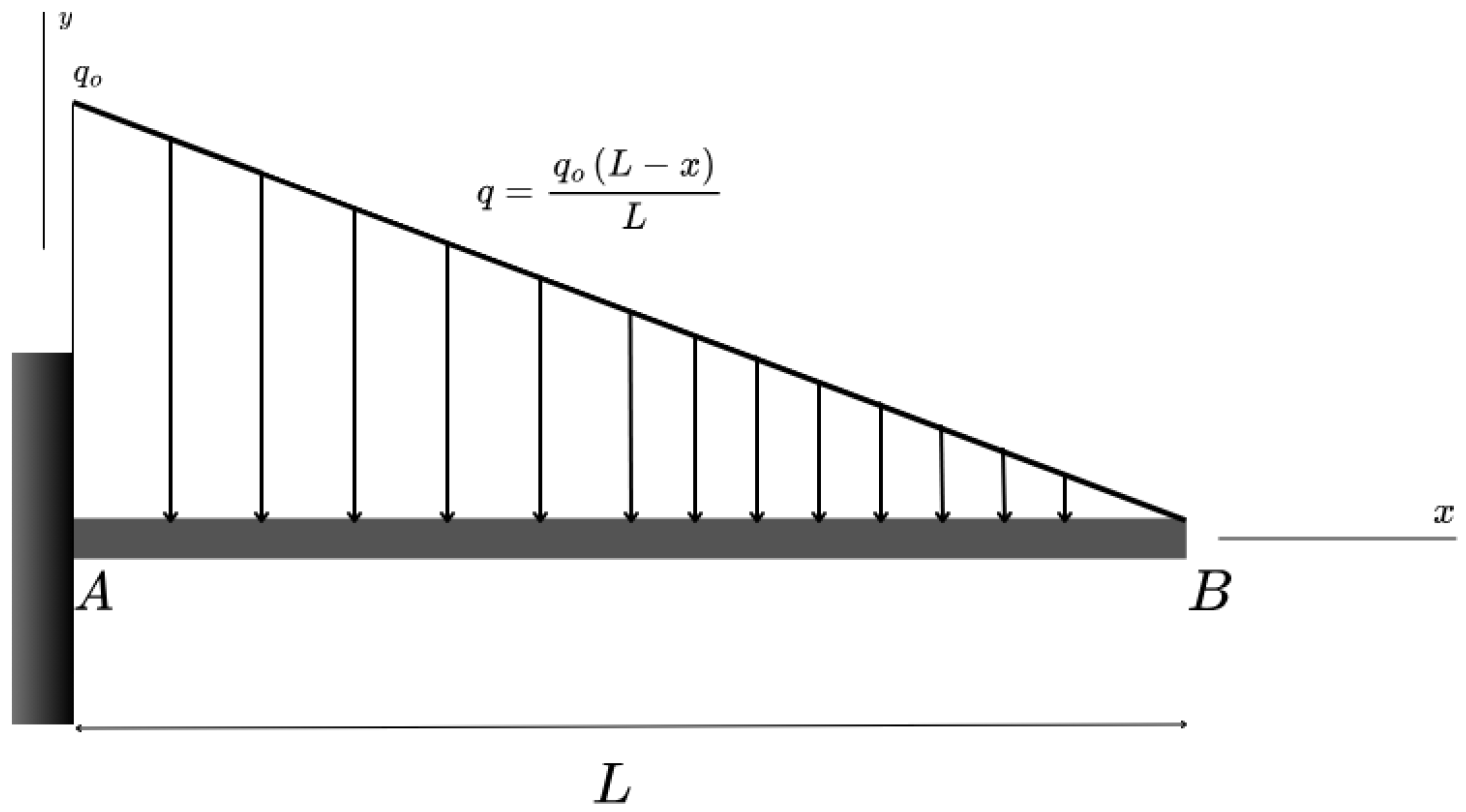
Figure 3. Cantilever Beam with Triangular Loading.
Preprints 119088 g003
Figure 4. Points over the length of beam
Preprints 119088 g004
Figure 5. Loss Curve for the PINN model
Preprints 119088 g005
Figure 6. Comparing the solutions from PINN and ANN for predicting deflection.
Preprints 119088 g006
Figure 7. Comparing the solutions from PINN and ANN for predicting slope (a), bending moment (b), and shear force (c).
Preprints 119088 g007
Figure 8. Loss curve for the ANN Model
Preprints 119088 g008
Table 1. Neural Network Configuration
Epochs 300
Learning Rate 0.001
Optimizer Adam
Input Layer 1
Hidden Layers 5
Output Layer 1
Number of Neurons 50
Activation Function Tanh
Table 2. Comparison of MSE values between the exact and predicted solution for ANN and PINN model
ANN PINN
Deflection 3.070e-07 3.060e-09
Slope 4.500e-05 2.935e-08
Bending Moment 0.002 5.517e-08
Shear Force 0.049 1.127e-07
Disclaimer/Publisher’s Note: The statements, opinions and data contained in all publications are solely those of the individual author(s) and contributor(s) and not of MDPI and/or the editor(s). MDPI and/or the editor(s) disclaim responsibility for any injury to people or property resulting from any ideas, methods, instructions or products referred to in the content.
Copyright: This open access article is published under a Creative Commons CC BY 4.0 license, which permit the free download, distribution, and reuse, provided that the author and preprint are cited in any reuse.
Prerpints.org logo

Preprints.org is a free preprint server supported by MDPI in Basel, Switzerland.

Subscribe

© 2024 MDPI (Basel, Switzerland) unless otherwise stated