Preprint
Article
The Impact of Data Packet Loss on Neural Decoding
Altmetrics
Downloads
60
Views
37
Comments
0
This version is not peer-reviewed
Submitted:
24 September 2024
Posted:
24 September 2024
You are already at the latest version
Alerts
Abstract
Background: In the field of brain-computer interfaces, neural decoding plays a crucial role in translating neural signals into meaningful physical actions. These signals are transmitted to processors for decoding via wired or wireless channels, often encountering data loss, commonly referred to as "packet loss." Despite its importance, the impact of different types and degrees of packet loss on neural decoding has yet to be comprehensively studied. Understanding this impact is critical for advancing neural signal processing and data filtering.
Methods: This paper addresses this gap by constructing four distinct packet loss models, simulating congestion packet loss, distributed packet loss, and burst packet loss scenarios. Using macaque superior arm-movement decoding experiments, we evaluate the effects of these packet loss types on decoding performance.
Results: Our findings reveal that continuous burst packet loss significantly degrades decoding performance at the same packet loss probability, and decoding parameters that are sensitive to data continuity are more heavily impacted by packet loss.
Conclusions: This study provides an analysis of the relationship between packet loss and neural decoding results, offering valuable insights for future strategies aimed at preventing and handling packet loss in neural signal acquisition.
Keywords:
Subject: Engineering - Bioengineering
1. Introduction
Neural decoding technology plays a critical role in brain-computer interface (BCI) research. By analyzing neural signals, researchers can extract information about the subject’s intentions or movements, enabling brain-controlled operations. Over the past few decades, neural decoding has enabled various interpretations, such as motion decoding [1,2,3] and language decoding [4,5]. This technology holds significant potential in the diagnosis, treatment, and rehabilitation of neurological diseases [6,7,8].
Neural signal acquisition, as the primary data source for neural decoding technology, is vital to the overall effectiveness of decoding. The transmission media used in neural signal acquisition can be categorized into two types: wired and wireless. Wired transmission offers higher bandwidth and more channels, making it the most commonly used method in current applications. However, wireless transmission is free from cable interference, enabling greater freedom of movement for the subject, which is particularly advantageous in experimental studies involving free motion. As research into the nervous system progresses, lightweight and flexible wireless brain-computer interface systems are gaining increasing attention from researchers due to their practical benefits and versatility.
Between the recording and decoding of neural signal data, packet loss is inevitable, whether using wired or wireless transmission modes. When the device configuration is correct, the physical reasons for packet loss may include network congestion and line interference [9,10]. Compared to wired transmission, wireless transmission are more susceptible to external interference, and considering factors such as power consumption, size, and transmission distance, the data transmission bandwidth is smaller compared to wired transmission. The wireless neural signal acquisition and transmission system developed by related neuroscience instrument companies and research teams has gradually been promoted in the field of neuroscience research, such as CerePlex W(Blackrock Neurotech, USA), the results and processing methods related to data packet loss have been mentioned in some studies. Berger et al. [11] have used two 96-channel Exilis Headstages(Blackrock Neurotech, USA) to record neural signals from monkeys wirelessly. In their experiment, the best session showed loss rates of 1.03%, and the worst session of 6.59%, respectively. They believe that experimental results bias was introduced by trials with high data loss rates. When removing trials with a loss rate of above 5% there was no significant bias anymore. Lee et al. [12] have developed wireless recording system could stably transmit neural data to the server, the packet loss rate is approximately 3%. Packet losses can occur randomly, but most of the causes were from crosstalk with other nearby wireless communication systems. Simeral et al. [13] have used four components provided by Blackrock Neurotech to record neural signals from participants: a pedestal-mounted wireless transmitter, four polarized planar antennas, a wireless receiver and a digital hub. This device achieves a minimum packet loss of 0.4166% and a maximum packet loss of 4.69%. Due to the use of multiple transmitters, a large number of packet losses on one transmitter have little impact on the final decoding result. Hansmeyer et al. [14] have also used 96-channel Exilis Headstages(Blackrock Neurotech, USA) to record neural signals from monkeys. They have reinforced the structure, with an average packet loss rate of 1.5% compared to previous studies. In current research, the packet loss rate of wireless devices is generally within 7%. Due to electromagnetic environment, device placement, and other conditions, the packet loss situation may be better or worse. However, there is currently a lack of quantitative research on the impact of packet loss on neural signal processing, especially subsequent neural decoding.
There are various reasons for packet loss in wireless transmission. In terms of specific manifestations, there are several types: Congestion loss. The packet loss will occur when the buffer overflows caused by the burst of data traffic [15,16,17]. This type of packet loss is specifically manifested as the loss of continuous large segments of data packets. Distributed loss. This type of packet loss often occurs in situations such as signal interference and equipment failure. In terms of statistical probability, this type of packet loss is more likely to the average distribution [18,19,20]. Burst loss. This type of packet loss is mostly continuous, meaning that once a packet loss occurs, several packet losses will occur. Unlike congestion loss, this type of packet loss is still probabilistic. Currently, most studies use the Gilbert-Elliott model(GE model) to investigate burst loss [21,22,23].It is widely believed that packet loss will have an impact on subsequent data processing. However, in the field of neural signal decoding, there is a lack of quantitative analysis on the decoding results caused by data packet loss, especially the impact of different types of packet loss on neural decoding. In most studies, the processing method for data with packet loss is to directly discard it. In this study, we constructed four different types of packet loss models and used macaque superior arm-movement decoding experiments [24] to verify the impact of packet loss on decoding results. The results indicate that different types of packet loss have significant differences in their impact on decoding results, providing reference for other studies on packet loss prevention, the impact of packet loss, and the processing of packet loss data.
2. Materials and Methods
2.1. Signal Acquisition
The neural data utilized in this study were sourced from a publicly available dataset provided by the Sabes lab. [25] These data were recorded from both the M1 and S1 areas of a macaque during the performance of a behavioral task, which involved continuous self-paced reaching movements towards targets arranged in an 8×8 square grid using the right arm. The recordings were made using a 96-channel intracranial micro-electrode array. This study used all 37 sessions of data from the monkey Indy, spanning approximately 10 months and encompassing a total of 20,000 reaching movements.
2.2. Signal Processing
The recurrent exponential-family harmonium (rEFH) [26] is a novel filter introduced by Philip N. Sabes to address the limitations of the Kalman filter algorithm [27], which is widely used in neural decoding. For the data mentioned above, rEFH outperforms some of the most frequently used decoding algorithms. This study select rEFH as the neural decoding algorithm to analyze the effects of packet loss.
Prior to commencing neural network training, it is essential to perform several preprocessing steps on the raw data extracted from the dataset to enhance its manageability and facilitate subsequent processing. As shown in Figure 1(a), the raw neural data is structured in a 192×3 cell array, where the 192 rows correspond to 192 channels from the M1 and S1 areas of the monkey, and the 3 columns represent three distinct spike signal types. Each cell contains a matrix with dimensions N×1, where each entry denotes the time at which a spike signal occurs.
As the first step, we consider neural pathways rather than physical channels, implying that neural signals passing through the same physical channel may originate from different neural pathways. Consequently, the original cell array is transformed into a 576×1 cell array, where the 576 rows represent the 576 neural pathways. As shown in Figure 1(b).
The next step is to construct a new matrix based on the time information in each cell. By defining a time interval, we can count the number of spikes occurring within each interval for each neural channel. This results in a matrix with dimensions N×576, where the nth row represents the nth time interval, and the 576 columns correspond to the 576 neural pathways. Each element in the matrix represents the number of spikes observed in a single neural pathway during a given time interval. As shown in Figure 1(c).
This matrix serves as the foundation for initiating neural network training, using both the spike data and location information provided in the dataset. Additionally, a packet loss model can be incorporated to simulate the effects of actual packet loss on the neural pathways.
2.3. Packet Loss Model
After the preprocessing steps After completing the preprocessing of the raw data, we obtained a matrix that next all named matrix A with dimensions N×576. At this stage, various packet loss models can be applied to this matrix to simulate the effects of actual packet loss on the data. As shown in Figure 2.
2.3.1. Congestion Loss
Congestion packet loss often occurs when the amount of data in a transmission exceeds the bandwidth of the data transmission, which can lead to a large amount of data loss in the excess of the bandwidth. To simulating this type of packet loss, we first calculate the total number of spikes X for each row i in the matrix A:
where represents the spike count in the jth channel during the ith time interval, and N is the total number of channels. If exceeds the bandwidth Z, which corresponds to the number of packets exceeding the bandwidth at a given time interval. All channel spike signals in the interval will be sorted from early to late, assuming that the sorting results are , which j represents the channel and k denotes the random ordering of spike signals for this channel. With the sorting result, we can simulate the congestion loss mode using the following formula:
This process is repeated until all rows have been traversed, resulting in the modified matrix A’.
2.3.2. Distributed Loss
According to the different ways of data packaging, distributed packet loss can also be categorized into two types, full package loss and single package loss.
The full packet loss model assumes that neural signals are transmitted in discrete, complete packet formats. When packet loss occurs in this transmission mode, all neural signal data within the affected packet is lost. In the resulting matrix A, each row represents a complete packet of spike data.
To simulate the full packet loss model within the neural signal matrix A, we first calculate the total number of packets to be lost, denoted as L, using the following formula:
where p represents the packet loss rate, and N corresponds to the total number of rows in matrix A. Subsequently, we randomly select L rows from the matrix using the MATLAB function randperm, and set their values to zero, thereby simulating the full packet loss model. The resulting matrix, denoted as A’, reflects the impact of the packet loss, with the selected rows zeroed out.
The single package loss assumes that neural signals are transmitted alone. In order to simulate packet loss within the neural signal matrix A, we first calculate the total number of packets to be lost L as:
where p represents the packet loss rate. Subsequently, we randomly select elements within the matrix and decrement their values by 1, provided that > 0. This process is repeated until L packets have been lost, resulting in the modified matrix A’.
2.3.3. Burst Loss
The GE model was applied to simulate packet loss in the neural signal matrix A. This model operates based on a two-state Markov process, where each state represents a different packet transmission state: ’good’ (no loss) and ’bad’ (packet loss). The transition between the states can be described by the following equation:
Where denotes the state of the transition at time t, represents the state at the subsequent time step. During the ’bad’ state, a portion of the signals in the corresponding rows of matrix A are set to zero, simulating packet loss. The resulting matrix A’ reflects the impact of packet loss modeled by the Gilbert-Elliott process.
2.4. Evaluation Indicator
The result of the refh algorithm contains six parameters. They are position XY, speed XY, and acceleration XY. They represent the reconstruction of the monkey’s motion information at the level of position, speed, and acceleration. The coefficient of determination is a commonly used metric in statistics and regression analysis to measure how well a regression model explains the variation in the data. Specifically, quantifies the proportion of variance in the observed data that is explained by the model’s predictions. The formula is given as:
In this formula, represents the model’s predicted values, x is the actual observed value, and denotes the expectation operator (i.e., the mean). The numerator represents the mean squared error (MSE) between the observed and predicted values, while the denominator represents the total variance of the observed data with respect to its mean.
By calculating the coefficient of determination , we obtain a value ranging between 0 and 1, where a value of 1 signifies that the model fully accounts for the variance in the data, while a value of 0 indicates that the model fails to explain any variance. In this study, we calculate between the six parameters of the refh algorithm results and the actual data. We employ to evaluate the impact of packet loss on neural decoding. A higher value corresponds to a reduced impact of packet loss.
3. Results
The rEFH algorithm generates six-dimensional outputs, including position (x, y), speed (x, y), and acceleration (x, y). By comparing the algorithm’s outputs with actual results and calculating the evaluation parameter, the impact of different packet loss models on the performance of the refh algorithm can be rigorously analyzed.
3.1. Results of Packet Loss Model Construction
The results of packet loss simulation are shown in Figure 3. The average packet loss rate of each model is controlled at 2%. For the single loss model, the packet loss rate remains consistent across time intervals, fluctuating within a narrow range of approximately 2%. In the full loss model, entire packets are dropped at random time intervals, with the points of packet loss scattered more unpredictably. For the congestion loss model, packet loss is concentrated within specific intervals, with loss rates generally staying below 40%, and most variations occur between 0 and 20%. The burst loss model shows a packet loss rate of 100% at random intervals; unlike the full loss model, these intervals are more continuous, with consecutive time periods where the loss rate remains at 100%.
3.2. The Impact of Different Packet Loss on Decoding Results
3.2.1. Congestion Loss
When the set Z is varied at larger values (corresponding to greater wireless transmission bandwidth), there is no significant change in the values representing the six parameters. However, as Z gradually decreases toward a critical threshold, the values for all six parameters exhibit a noticeable decline. The trends in for the different parameters are largely consistent as Z varies, with speed and acceleration being more significantly affected by changes in Z compared to the other parameters.
3.2.2. Distributed Loss
The representing the six parameters exhibit a decreasing trend as the packet loss rate increases. Among these, the value associated with the acceleration shows the most significant change due to packet loss, while the value corresponding to the position is the least affected.
Figure 5.
Curve representing the value of acceleration (X, Y) speed (X, Y) position (X, Y) with increasing packet loss rate under the whole packet loss model.
Figure 5.
Curve representing the value of acceleration (X, Y) speed (X, Y) position (X, Y) with increasing packet loss rate under the whole packet loss model.
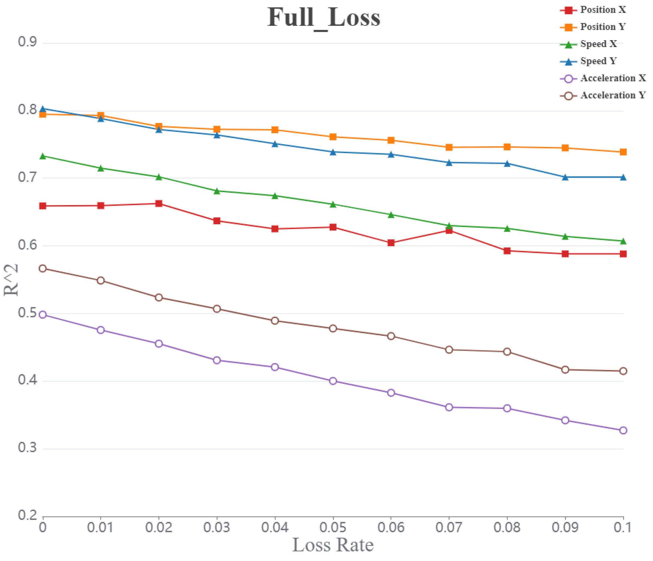
Figure 6.
Curve representing the value of acceleration (X, Y) speed (X, Y) position (X, Y) with increasing packet loss rate under the single loss model.
Figure 6.
Curve representing the value of acceleration (X, Y) speed (X, Y) position (X, Y) with increasing packet loss rate under the single loss model.
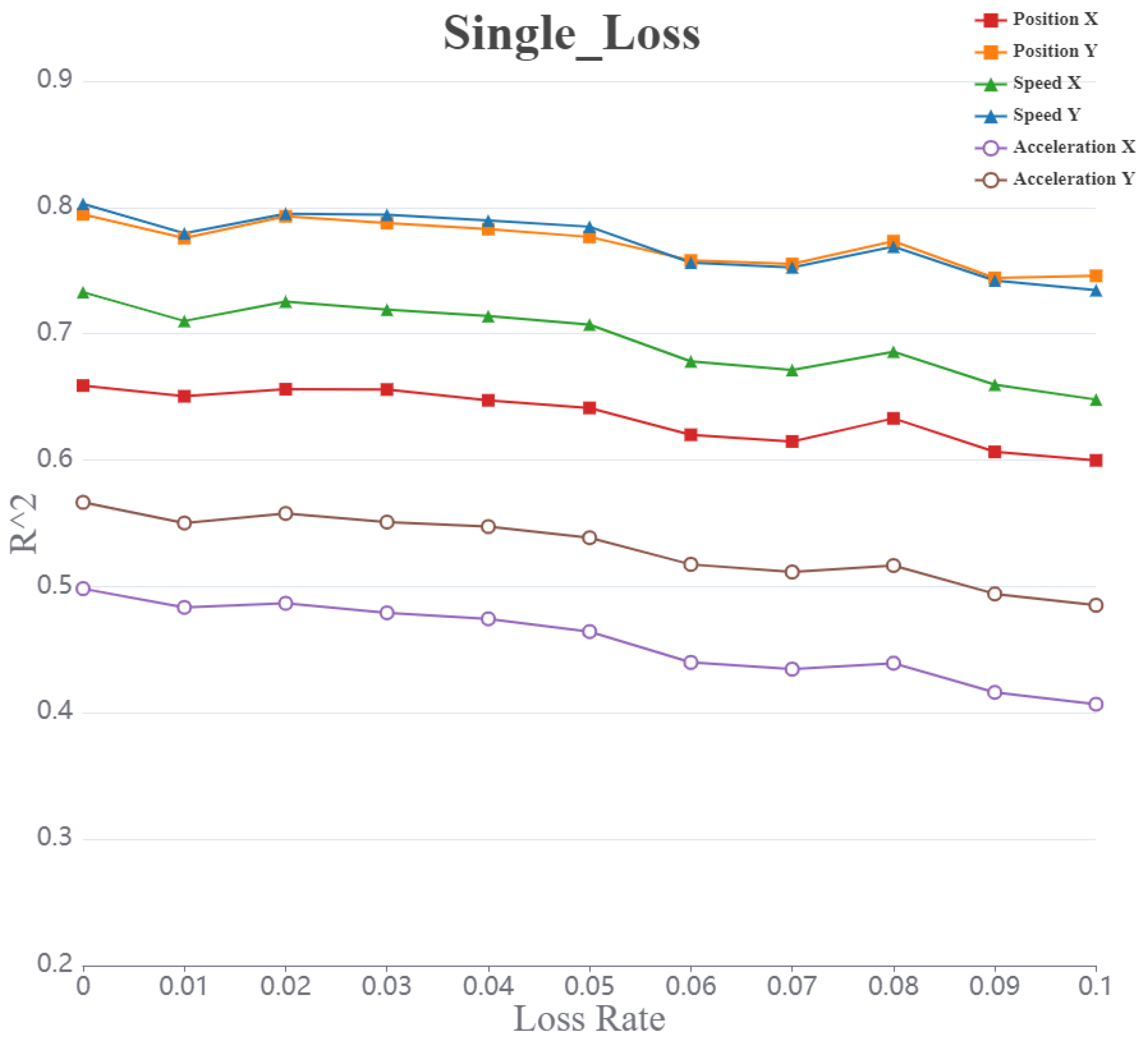
The values representing the six parameters decreased volatility as the packet loss rate increases. Among these, the value for acceleration shows the greatest change in magnitude, while the overall trend and magnitude of changes in the values for position and speed are similar.
3.2.3. Burst Loss
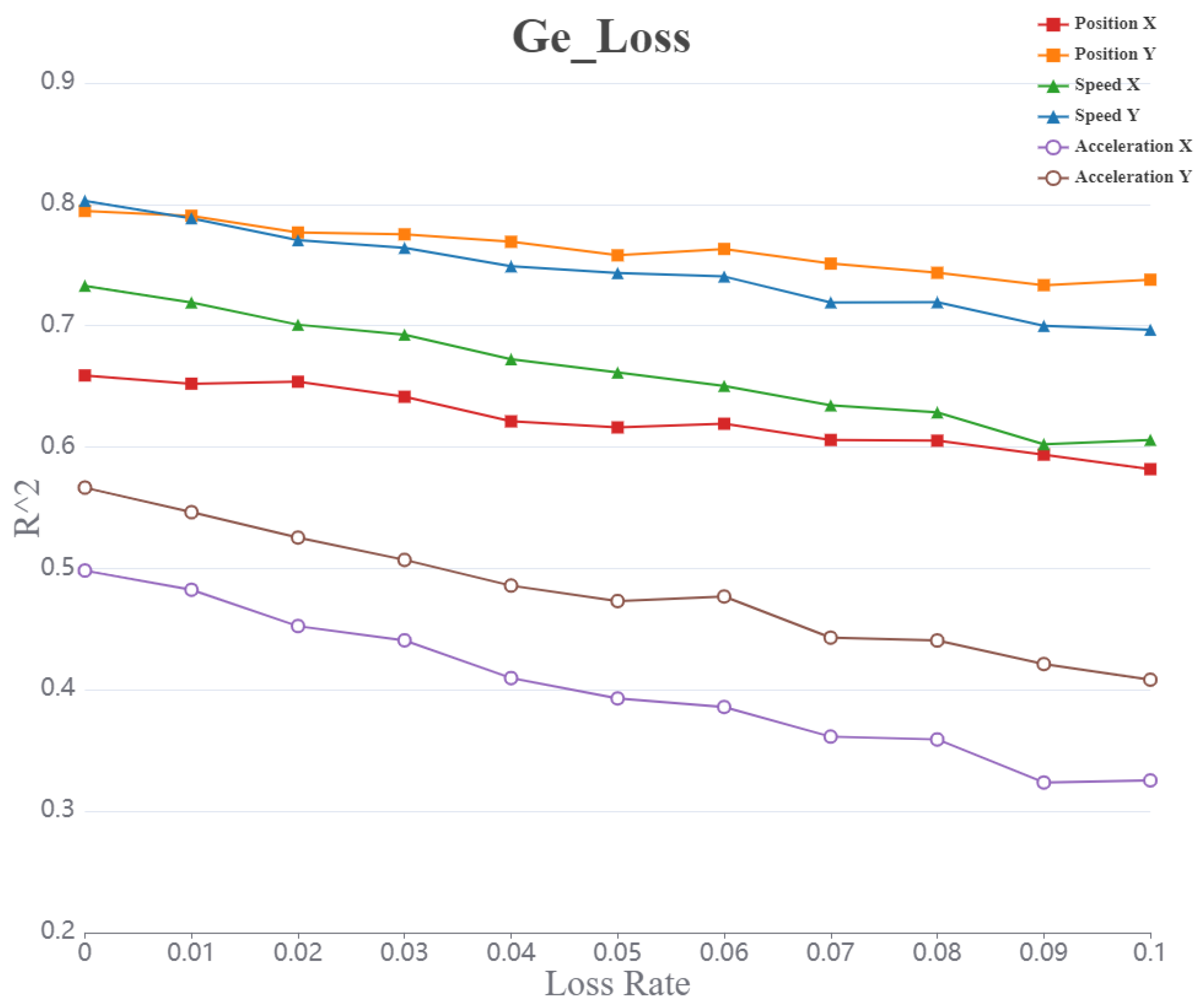
The values representing the six parameters all exhibit a gradual decline as the packet loss rate increases. Among them, the for acceleration shows the most significant change, while the values for position and speed follow similar overall trends and magnitudes.
Figure 7.
Curve representing the value of acceleration (X, Y) speed (X, Y) position (X, Y) under the GE packet loss model with increasing packet loss rate.
Figure 7.
Curve representing the value of acceleration (X, Y) speed (X, Y) position (X, Y) under the GE packet loss model with increasing packet loss rate.
3.3. Performance of Different Decoding Parameters on Packet Loss Data
The representing the position parameter XY exhibits a decreasing trend as the packet loss rate increases across different packet loss models. As shown in Figure 8(a). Under the full loss and burst models, the decline in is more gradual with increasing packet loss rate. In contrast, under the single loss model, shows a fluctuating downward trend, with occasional small increases as the packet loss rate rises. This suggests that the for parameter XY is least affected by the packet loss rate under the single loss model and most affected under the burst model. Furthermore, the values for parameters X and Y are similarly influenced by the various packet loss models, with the main difference observed under the full loss model. In this model, the representing parameter X demonstrates a more complex, fluctuating downward trend, while the representing parameter Y follows a more steady downward trajectory.
The values representing the speed parameter XY show an overall decreasing trend as the packet loss rate increases across different packet loss models. As shown in Figure 8(b). The overall decline is similar in both the full loss and burst loss models, with comparable rates of decrease. In contrast, the single loss model demonstrates a fluctuating but decreasing trend, with a smaller overall reduction compared to other packet loss models. Additionally, the decreasing trends of the speed parameters X and Y are largely consistent across the different models.
The representing the acceleration parameter exhibits a generally gentle decreasing trend as the packet loss rate increases across different packet loss models. As shown in Figure 8(c). The magnitude and trend of the decrease are nearly identical for both the full loss and burst loss models, whereas the single loss model shows a significantly smaller reduction compared to the other two models. The trends for both the acceleration parameter X and acceleration parameter Y are consistent across all packet loss models.
Among the position, speed, and acceleration parameters, the of the position parameter is the least impacted by packet loss, exhibiting the smallest overall decrease. In contrast, the of the acceleration parameter is the most affected by packet loss, with the largest overall reduction.
3.4. Reconstruction Result
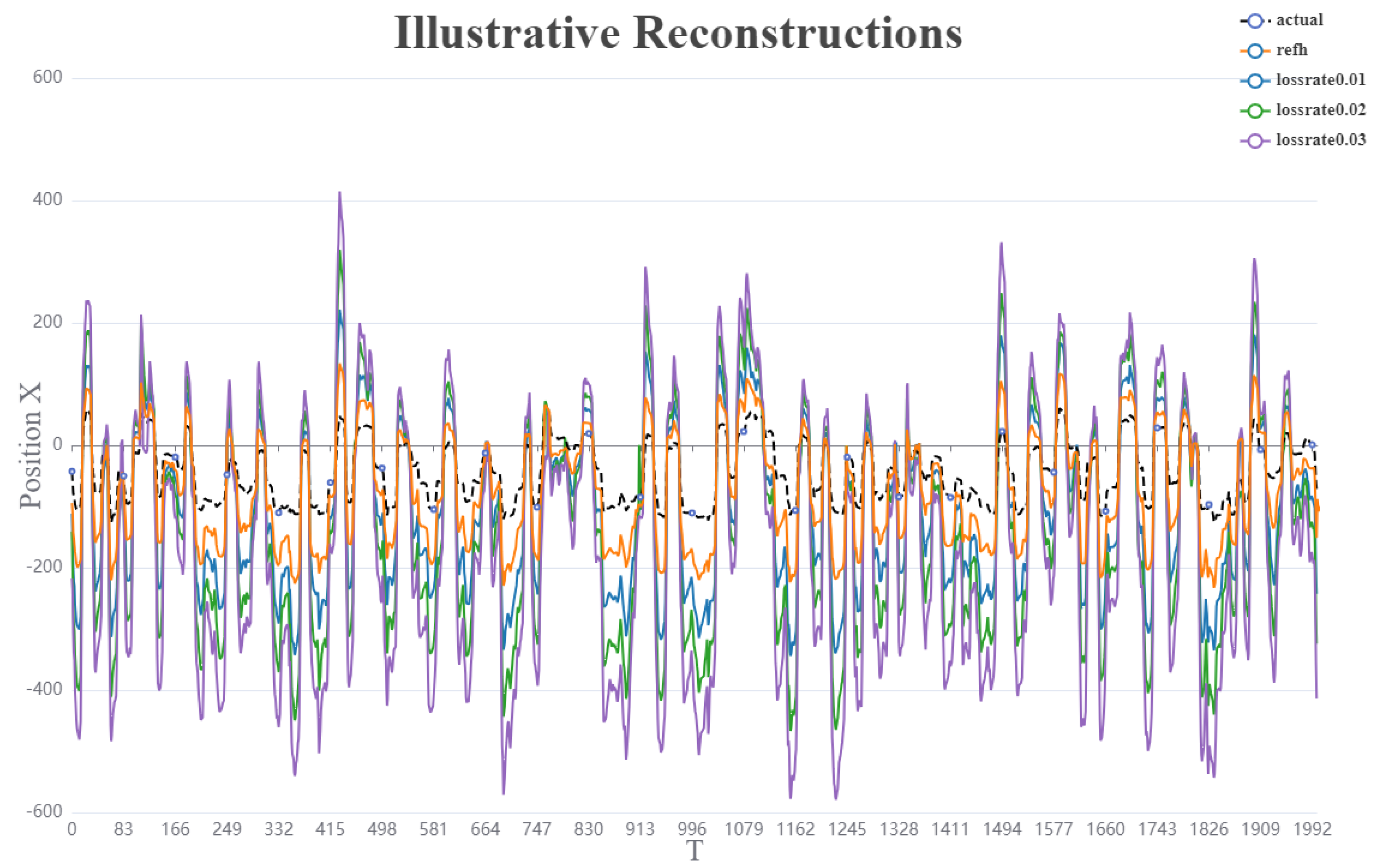
The overall reconstruction results indicate a clear trend: as the packet loss rate increases, the deviation of the position reconstruction in the X direction progressively grows. The reconstruction result that most closely aligns with the actual position is achieved by the rEFH algorithm without incorporating any packet loss model. Conversely, the result with the greatest deviation from the actual position is observed when the burst packet loss model, with a packet loss rate of 0.03, is applied. Despite variations in the degree of deviation across different packet loss rates, the overall trend of the reconstruction results remains consistent.
4. Discussion
In our study, we investigated the effects of various packet loss models on neural decoding outcomes. Specifically, we designed four distinct packet loss models, each based on different packing methods and wireless transmission characteristics. We applied these models to experimental data involving macaque reach kinematics for testing and analysis. Unlike previous studies that tended to discard data entirely when faced with significant packet loss, we took a different approach by analyzing and comparing how different types of packet loss affect decoding performance. This shift in methodology allows us to explore alternative strategies for dealing with lost data, offering insights into how different packet loss models impact the decoding process. Our findings highlight the importance of understanding the specific characteristics of packet loss, as different types of loss can have varying effects on the accuracy of the neural decoding process. This analysis provides important guidelines for handling packet loss in future neural signal processing and decoding applications, particularly in wireless systems where packet loss is inevitable.
4.1. Continuous and Burst Packet Loss Have Greater Impact on Decoding
Our analysis shows that the congestion loss model has a minimal impact on the decoding of position, speed, and acceleration in both the x and y directions. Even in scenarios with sufficient bandwidth, where ample spike information is available, the decoding performance remains stable, and ideal results can still be achieved despite packet loss caused by network congestion. Next is the single loss model. For the main experiments of this article, spikes were binned at 128ms intervals. the single loss model resulted in a reduction of spike counts in every bin, though the complete loss of an entire bin was exceedingly rare. This ensures that the continuity of the neural signals along the timeline is largely preserved. In contrast, the full loss model, which results in the loss of complete data bins, disrupts data continuity. Even when the total number of lost bits is similar, the loss of entire data packets leads to poorer decoding performance compared to the single loss model. A key insight from these results is the importance of designing data packaging strategies that minimize the size of the data units being transmitted. By reducing the packet size, we can avoid the complete loss of packets, thus preserving the continuity of neural signals and improving decoding performance. However, this approach comes with trade-offs. Smaller packets require additional metadata (such as headers, tails, and checksum) for transmission, which reduces overall efficiency and increases bandwidth usage. Therefore, it is crucial to strike a balance between packaging size and transmission efficiency.
The GE loss model more closely approximates real-world conditions, and it demonstrates how disruptions in data continuity significantly impact decoding performance. In the GE model, transitions between Good and Bad states affect the integrity of the transmitted data. To mitigate the impact of packet loss, it is essential to decrease the transition probability from the Good state to the Bad state, while simultaneously increasing the probability of returning from a Bad state to a Good state. The primary strategy is to enhance transmission quality to reduce the likelihood of entering a Bad state. However, if a transition to the Bad state occurs, minimizing packet loss and rapidly returning to the Good state is critical. This can be achieved through various techniques, including:Automatic Retransmission Requests (ARQ) [28]: Requests to resend lost packets. Forward Error Correction (FEC) [29]: Adding redundancy to the data stream to enable recovery of lost packets without retransmission. Transmission Rate Adjustment: Dynamically adjusting the transmission rate to adapt to network conditions and reduce packet loss. By applying these strategies, we can reduce the detrimental effects of packet loss and maintain higher neural decoding accuracy, especially in systems where data continuity is crucial.
4.2. Decoding with Higher Data Continuity Requirements Is More Affected by Packet Loss
In this decoding experiment, spike counts are a linear function of these variables as well as the six kinematic states themselves [25]. Due to the sparsity of the processed spike count matrix and the relatively slow changes in position compared to speed and acceleration, small amounts of packet loss have a minimal impact on position decoding.
However, since speed and acceleration are derivatives of position and depend on the dynamic discharge patterns in neural signals over short time intervals, packet loss or signal discontinuities can directly affect the accuracy of these estimates. This is because the derivatives amplify any fluctuations or inconsistencies in the underlying signal. Additionally, the recursive nature of the decoding algorithm can exacerbate errors in speed and acceleration estimation, leading to the accumulation of prediction errors. These accumulated errors further degrade decoding performance, especially for speed and acceleration, which are highly sensitive to small temporal changes. As a result, neural decoding algorithms that demand high data continuity and integrity are particularly sensitive to packet loss. In contrast, algorithms based on sparse matrices or averaged spike rate data may exhibit slightly better tolerance to packet loss due to the smoother or less dynamic nature of the data being processed.
4.3. The Relationship between Packet Loss Rate and Decoding Result
The accuracy requirements for decoding results vary depending on the evaluation criteria and the specific application scenarios. For example, in the rat compression bar experiment [30], the goal is to determine whether the bar has been pressed, a binary classification task. In such cases, high decoding accuracy may not be essential, and the system can tolerate a certain amount of packet loss without significantly affecting performance.
In contrast, for trajectory prediction tasks, such as the experiment presented in this study, the ideal scenario is for the decoded motion trajectory to perfectly match the actual trajectory—an outcome where the is 1. However, no existing decoding algorithm can achieve such a high performance metric. Thus, in regression tasks like this, it is crucial to minimize packet loss to maximize decoding accuracy.
In this study, we found that a packet loss of less than 2% can ensure that the difference in values between the predicted trajectory and the true trajectory is within 0.05. Additionally, the impact of packet loss on position decoding was found to be slightly smaller compared to speed and acceleration.
This study has several limitations:
Firstly, given the high precision required in kinematic decoding, the analysis was limited to one specific kinematic experimental paradigm. However, the packet loss model developed here can also be applied to other forms of neural decoding, broadening its potential use in future studies.
Secondly, the evaluation metrics for assessing the impact of packet loss on decoding results lack universality. Currently, the impact is gauged through performance indicators such as decoding accuracy or trajectory similarity, which vary across different decoding algorithms. This variation complicates the subsequent processing of packet loss data, as each algorithm requires tailored evaluation criteria. Developing more universal metrics or models could streamline the process of data filtering and handling in future research.
5. Conclusions
This study examines the impact of packet loss on neural signal decoding by constructing four distinct packet loss models. Our results show that, under the same packet loss probability, continuous burst packet loss has a more significant negative effect on decoding performance, suggesting the necessity of prevention strategies like packet retransmission. On the other hand, occasional packet loss has a comparatively minor effect on decoding results within certain limits. The insights and models presented here offer valuable references for addressing packet loss in future neural signal acquisition processes, particularly in wireless transmission environments where packet loss is more prevalent.
Author Contributions
Conceptualization, X.G. and F.Z.; methodology, X.G. and J.Z.; software, J.Z.; validation, Q.S. and L.C.; formal analysis, F.W. and B.G.; investigation, Q.S.; resources, Y.L.; data curation, J.Z.; writing—original draft preparation, J.Z.; writing—review and editing, X.G.; visualization, Y.L.; supervision, F.Z.; project administration, X.G.; funding acquisition, X.G. All authors have read and agreed to the published version of the manuscript.
Funding
This research was funded by the grant from National Key R&D Program of China (2021ZD0200405), the China Postdoctoral Science Foundation under Grant Number 2024M752811 and Key Agricultural and Social Development Projects of Hangzhou(202204A09).
Institutional Review Board Statement
Not applicable.
Informed Consent Statement
Not applicable
Data Availability Statement
The data presented in this study are available in zenodo at https://doi.org/10.5281/ zenodo.3854034.
Conflicts of Interest
The authors declare no conflicts of interest.
References
- Willett, F.R.; Avansino, D.T.; Hochberg, L.R.; Henderson, J.M.; Shenoy, K.V. High-performance brain-to-text communication via handwriting. NATURE 2021, 593, 249. [Google Scholar] [CrossRef] [PubMed]
- Shah, N.P.; Willsey, M.S.; Hahn, N.; Kamdar, F.; Avansino, D.T.; Hochberg, L.R.; Shenoy, K.V.; Henderson, J.M. A brain-computer typing interface using finger movements. In Proceedings of the 2023 11TH INTERNATIONAL IEEE/EMBS CONFERENCE ON NEURAL ENGINEERING, NER, 2023, International IEEE EMBS Conference on Neural Engineering. [CrossRef]
- Casey, A.; Azhar, H.; Grzes, M.; Sakel, M. BCI controlled robotic arm as assistance to the rehabilitation of neurologically disabled patients. DISABILITY AND REHABILITATION-ASSISTIVE TECHNOLOGY 2021, 16, 525–537. [Google Scholar] [CrossRef] [PubMed]
- Metzger, S.L.; Littlejohn, K.T.; Silva, A.B.; Moses, D.A.; Seaton, M.P.; Wang, R.; Dougherty, M.E.; Liu, J.R.; Wu, P.; Berger, M.A.; et al. A high-performance neuroprosthesis for speech decoding and avatar control. NATURE 2023, 620, 1037. [Google Scholar] [CrossRef] [PubMed]
- Kobayashi, N.; Morooka, T. Application of High-accuracy Silent Speech BCI to Biometrics using Deep Learning. In Proceedings of the 2021 9TH IEEE INTERNATIONAL WINTER CONFERENCE ON BRAIN-COMPUTER INTERFACE (BCI); International Winter Workshop on Brain-Computer Interface, 2021; pp. 138–143. [Google Scholar] [CrossRef]
- Pels, E.G.M.; Aarnoutse, E.J.; Leinders, S.; Freudenburg, Z.V.; Branco, M.P.; van der Vijgh, B.H.; Snijders, T.J.; Denison, T.; Vansteensel, M.J.; Ramsey, N.F. Stability of a chronic implanted brain-computer interface in late-stage amyotrophic lateral sclerosis. CLINICAL NEUROPHYSIOLOGY 2019, 130, 1798–1803. [Google Scholar] [CrossRef] [PubMed]
- Mane, R.; Chouhan, T.; Guan, C. BCI for stroke rehabilitation: motor and beyond. JOURNAL OF NEURAL ENGINEERING 2020, 17. [Google Scholar] [CrossRef] [PubMed]
- Abtahi, M.; Borgheai, S.B.; Jafari, R.; Constant, N.; Diouf, R.; Shahriari, Y.; Mankodiya, K. Merging fNIRS-EEG Brain Monitoring and Body Motion Capture to Distinguish Parkinsons Disease. IEEE TRANSACTIONS ON NEURAL SYSTEMS AND REHABILITATION ENGINEERING 2020, 28, 1246–1253. [Google Scholar] [CrossRef] [PubMed]
- Mishra, T.K.; Sahoo, K.S.; Bilal, M.; Shah, S.C.; Mishra, M.K. Adaptive Congestion Control Mechanism to Enhance TCP Performance in Cooperative IoV. IEEE ACCESS 2023, 11, 9000–9013. [Google Scholar] [CrossRef]
- Akasaka, H.; Hakamada, K.; Morohashi, H.; Kanno, T.; Kawashima, K.; Ebihara, Y.; Oki, E.; Hirano, S.; Mori, M. Impact of the suboptimal communication network environment on telerobotic surgery performance and surgeon fatigue. PLOS ONE 2022, 17. [Google Scholar] [CrossRef] [PubMed]
- Berger, M.; Agha, N.S.; Gail, A. Wireless recording from unrestrained monkeys reveals motor goal encoding beyond immediate reach in frontoparietal cortex. ELIFE 2020, 9. [Google Scholar] [CrossRef] [PubMed]
- Lee, K.J.; Hong, D.; Jang, J.W.; Lee, K.Y.; Park, B.; Kim, J.H.; Kim, J.S.; Kim, S. A Wireless ECoG Recording System to Detect Brain Responses to Tactile Stimulation. IEEE SENSORS JOURNAL 2023, 23, 13692–13701. [Google Scholar] [CrossRef]
- Simeral, J.D.; Hosman, T.; Saab, J.; Flesher, S.N.; Vilela, M.; Franco, B.; Kelemen, J.N.; Brandman, D.M.; Ciancibello, J.G.; Rezaii, P.G.; et al. Home Use of a Percutaneous Wireless Intracortical Brain-Computer Interface by Individuals With Tetraplegia. IEEE TRANSACTIONS ON BIOMEDICAL ENGINEERING 2021, 68, 2313–2325. [Google Scholar] [CrossRef] [PubMed]
- Hansmeyer, L.; Yurt, P.; Agha, N.; Trunk, A.; Berger, M.; Calapai, A.; Treue, S.; Gail, A. Home-Enclosure-Based Behavioral and Wireless Neural Recording Setup for Unrestrained Rhesus Macaques. ENEURO 2023, 10. [Google Scholar] [CrossRef] [PubMed]
- Hou, Y.; He, H.; Jiang, X.; Chen, S.; Yang, J. Deep-Reinforcement-Learning-Aided Loss-Tolerant Congestion Control for 6LoWPAN Networks. IEEE INTERNET OF THINGS JOURNAL 2023, 10, 19125–19140. [Google Scholar] [CrossRef]
- Xing, X.; Yang, S.; Ji, X.; Peng, S. Optimization of TCP Congestion Control Algorithms Loss-Based in Wireless Network. In Proceedings of the EMERGING NETWORKING ARCHITECTURE AND TECHNOLOGIES, ICENAT 2022; Quan, W., Ed. Peng Cheng Lab, 2023, Vol. 1696, Communications in Computer and Information Science, pp. 381–392. 1st International Conference on Emerging Networking Architecture and Technologies (ICENAT), ELECTR NETWORK, NOV 15-17, 2022. [CrossRef]
- Chen, Y.; Yan, J.; Zhang, Y.; Hummel, K.A. Differentiating Losses in Wireless Networks: A Learning Approach. In Proceedings of the IEEE INFOCOM 2022 - IEEE CONFERENCE ON COMPUTER COMMUNICATIONS WORKSHOPS (INFOCOM WKSHPS). IEEE, 2022, IEEE Conference on Computer Communications Workshops. IEEE Conference on Computer Communications (IEEE INFOCOM), ELECTR NETWORK, MAY 02-05, 2022. [CrossRef]
- Lin, C.H.; Ke, C.H.; Shieh, C.K.; Chilamkurti, N.K. The packet loss effect on MPEG video transmission in wireless networks. In Proceedings of the 20TH INTERNATIONAL CONFERENCE ON ADVANCED INFORMATION NETWORKING AND APPLICATIONS, VOL 1, PROCEEDINGS, 2006, pp. 565+.
- Shi, Y.; Fang, X.; Wang, J.; Gu, S.; Huang, Y. Robust H∞ Control for An Uncertain Wireless Sensor Networks Considering Random Delay and Packets-loss. In Proceedings of the PROCEEDINGS OF THE 32ND 2020 CHINESE CONTROL AND DECISION CONFERENCE (CCDC 2020), 2020, Chinese Control and Decision Conference, pp. 1409–1414.
- Han, S.; Wang, F. Research on Filtering for Random Data Packet Dropouts and Delays in Wireless Sensor Networks. In Proceedings of the ICAROB 2018: PROCEEDINGS OF THE 2018 INTERNATIONAL CONFERENCE ON ARTIFICIAL LIFE AND ROBOTICS; Sugisaka, M.; Jia, Y.; Ito, T.; Lee, J., Eds., 2018, pp. 716–719.
- ELLIOTT, E. ESTIMATES OF ERROR RATES FOR CODES ON BURST-NOISE CHANNELS. BELL SYSTEM TECHNICAL JOURNAL 1963, 42, 1977. [Google Scholar] [CrossRef]
- Liu, F.; Luan, T.H.; Shen, X.S.; Lin, C. Dimensioning the packet loss burstiness over wireless channels: a novel metric, its analysis and application. WIRELESS COMMUNICATIONS & MOBILE COMPUTING 2014, 14, 1160–1175. [Google Scholar] [CrossRef]
- Palko, A.; Sujbert, L. FFT-Based Identification of Gilbert-Elliott Data Loss Models. IEEE TRANSACTIONS ON INSTRUMENTATION AND MEASUREMENT 2021, 70. [Google Scholar] [CrossRef]
- Makin, J.G.; O’Doherty, J.E.; Cardoso, M.M.B.; Sabes, P.N. Superior arm-movement decoding from cortex with a new, unsupervised-learning algorithm. JOURNAL OF NEURAL ENGINEERING 2018, 15. [Google Scholar] [CrossRef]
- O’Doherty, J.E.; Cardoso, M.M.B.; Makin, J.G.; Sabes, P.N. Nonhuman Primate Reaching with Multichannel Sensorimotor Cortex Electrophysiology, 2020. [CrossRef]
- Makin, J.; Dichter, B.; Sabes, P. Recurrent Exponential-Family Harmoniums without Backprop-Through-Time 2016. [CrossRef]
- Wu, W.; Gao, Y.; Bienenstock, E.; Donoghue, J.; Black, M. Bayesian population decoding of motor cortical activity using a Kalman filter. NEURAL COMPUTATION 2006, 18, 80–118. [Google Scholar] [CrossRef]
- Jung, Y.H.; Choi, J. Hybrid ARQ Scheme with Autonomous Retransmission for Multicasting in Wireless Sensor Networks. SENSORS 2017, 17. [Google Scholar] [CrossRef] [PubMed]
- Yu, J.; Liu, T.; Li, Y.; Ding, F.; Wu, S. On the Decoding Cost of Streaming Forward Erasure Correction Codes. IEEE COMMUNICATIONS LETTERS 2024, 28, 1760–1764. [Google Scholar] [CrossRef]
- Gao, H.; Qi, Y.; Zhang, F.; Sun, M.; Zhang, J.; Xu, K. Decoding Movements Using Local Field Potentials from Premotor Cortex of Stroke Rats. In Proceedings of the 2019 IEEE BIOMEDICAL CIRCUITS AND SYSTEMS CONFERENCE (BIOCAS 2019), 2019, Biomedical Circuits and Systems Conference. [CrossRef]
Figure 1.
(a) shows the original matrix derived from a publicly available dataset. In (b), data processing is applied, where the primary dimensional transformation treats each spike type as a separate channel, counting the number of spikes within a specified time interval. (c) illustrates the matrix after completing data processing, where each cell corresponds to the number of spikes in the respective channel during a particular time interval.
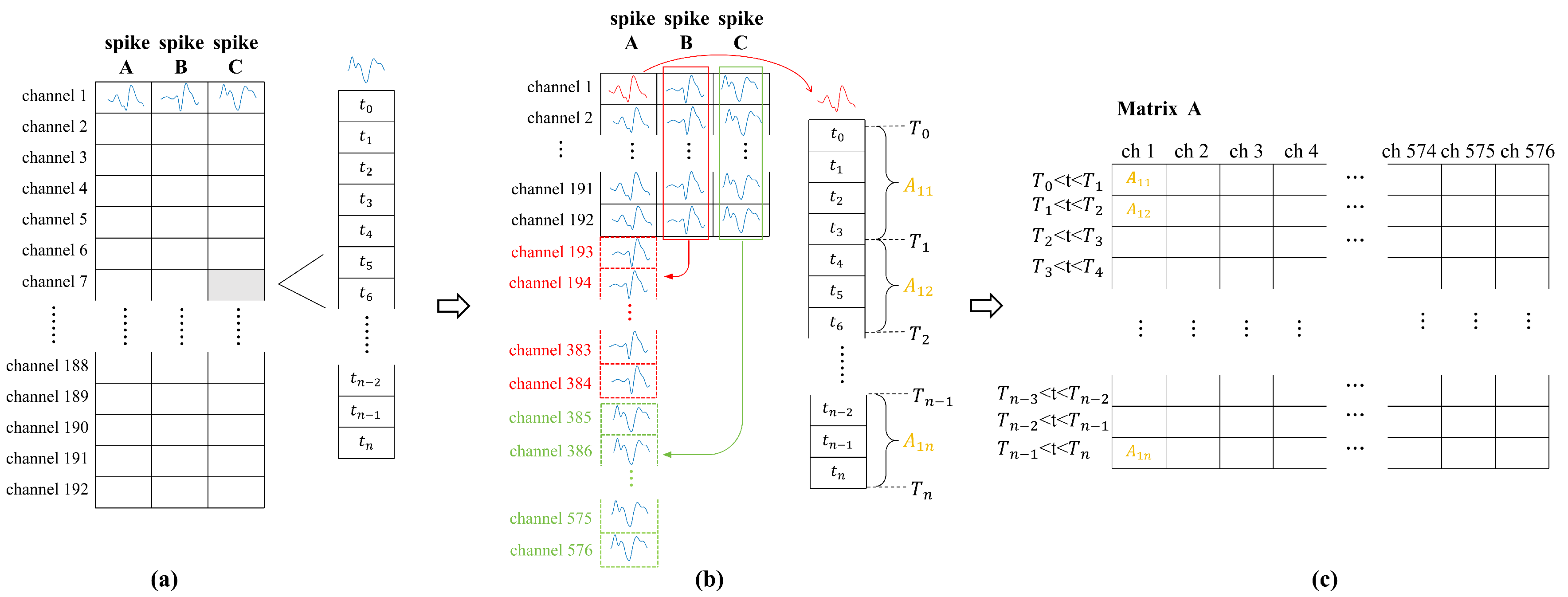
Figure 2.
(a) Congestion loss model: If the number of packets in a transmission exceeds the bandwidth limit Z(red dot line), the spike signals within that transmission are discarded once the cumulative time-ordered signals surpass the bandwidth threshold. (b) Single loss Model: This model randomly discards individual spike signals from the matrix, simulating isolated signal loss within the transmission. (c) Full loss model: This model considers all spike signals within a specific time interval as a single packet. The model randomly discards entire rows of spike data from the matrix, representing complete loss of information during transmission. (d) Burst loss model: This model simulates the state of wireless transmission under burst packet loss conditions. During favorable transmission states, no packet loss occurs. However, during unfavorable transmission states, entire rows of spike signals in the matrix are randomly dropped, mimicking burst loss events.
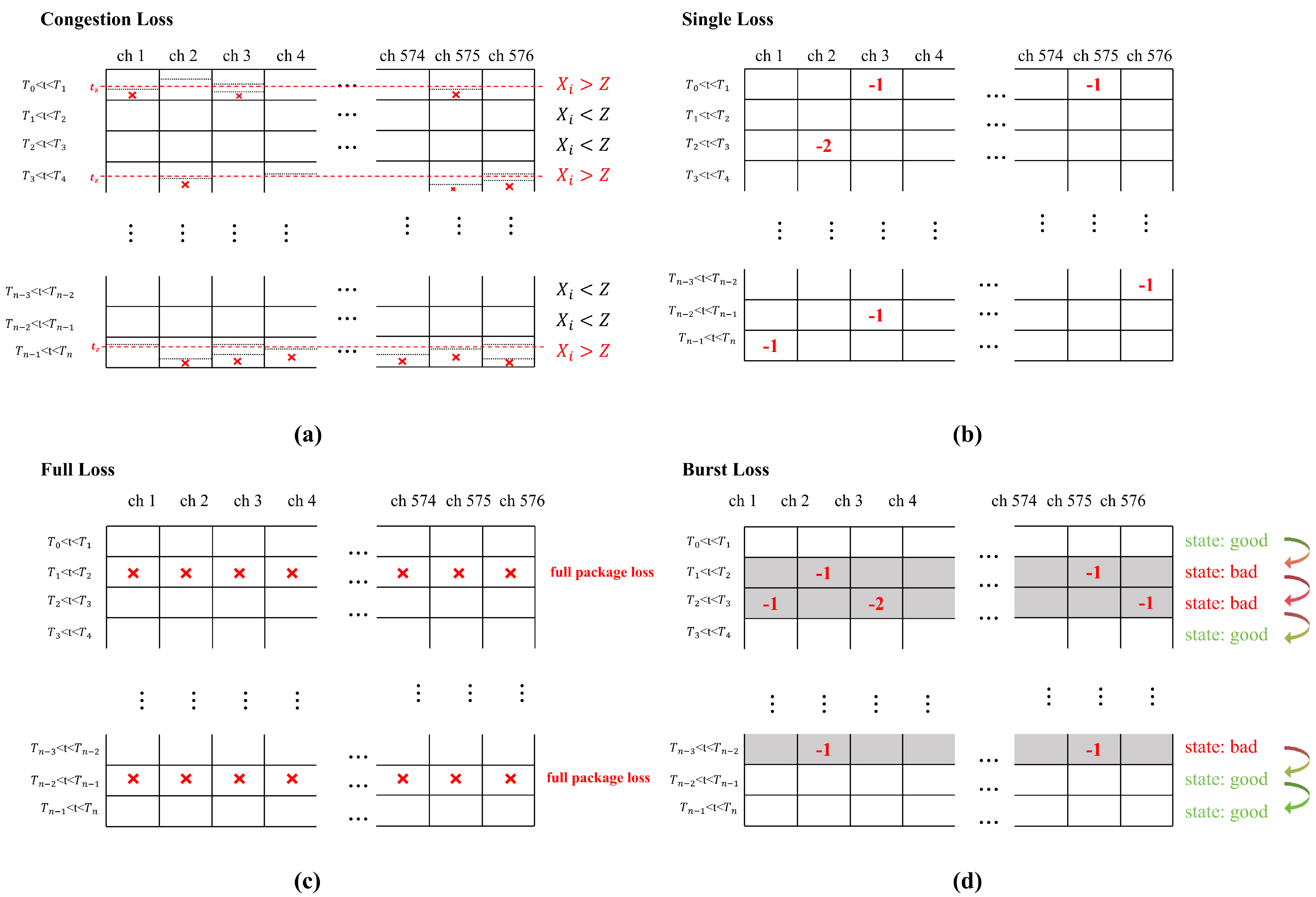
Figure 3.
The figure depicts the variation of packet loss rate over time , highlighting the behavior of four distinct packet loss models: burst loss, full loss, single loss, and congestion loss. The packet loss rate is plotted on the vertical axis, while time is represented on the horizontal axis. Each packet loss model is distinguished by a unique color, allowing for clear comparison of their respective trends over time.
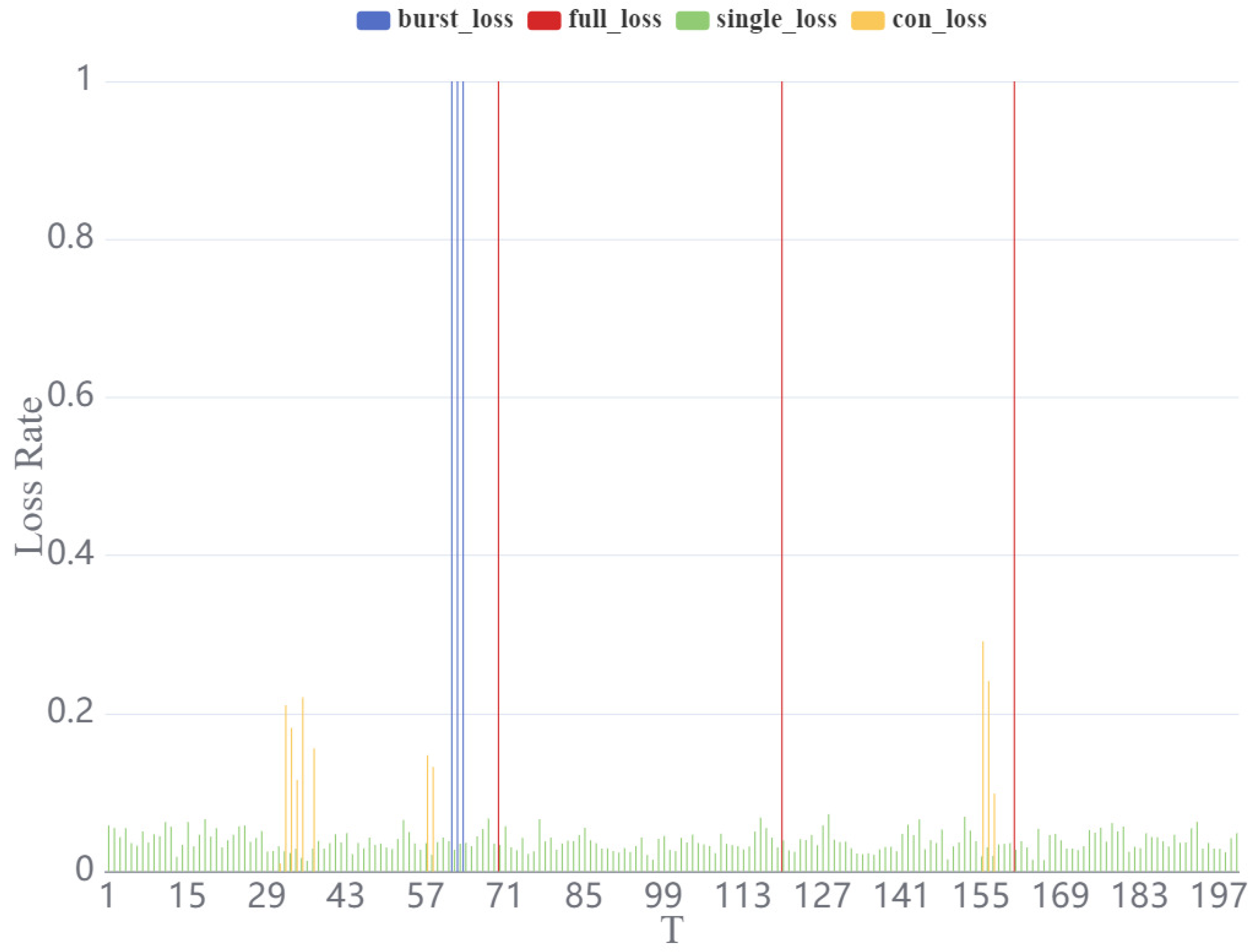
Figure 4.
Curve representing the value of acceleration (X, Y) speed (X, Y) position (X, Y) with decreasing bandwidth constraints under the congestion loss model.
Figure 4.
Curve representing the value of acceleration (X, Y) speed (X, Y) position (X, Y) with decreasing bandwidth constraints under the congestion loss model.
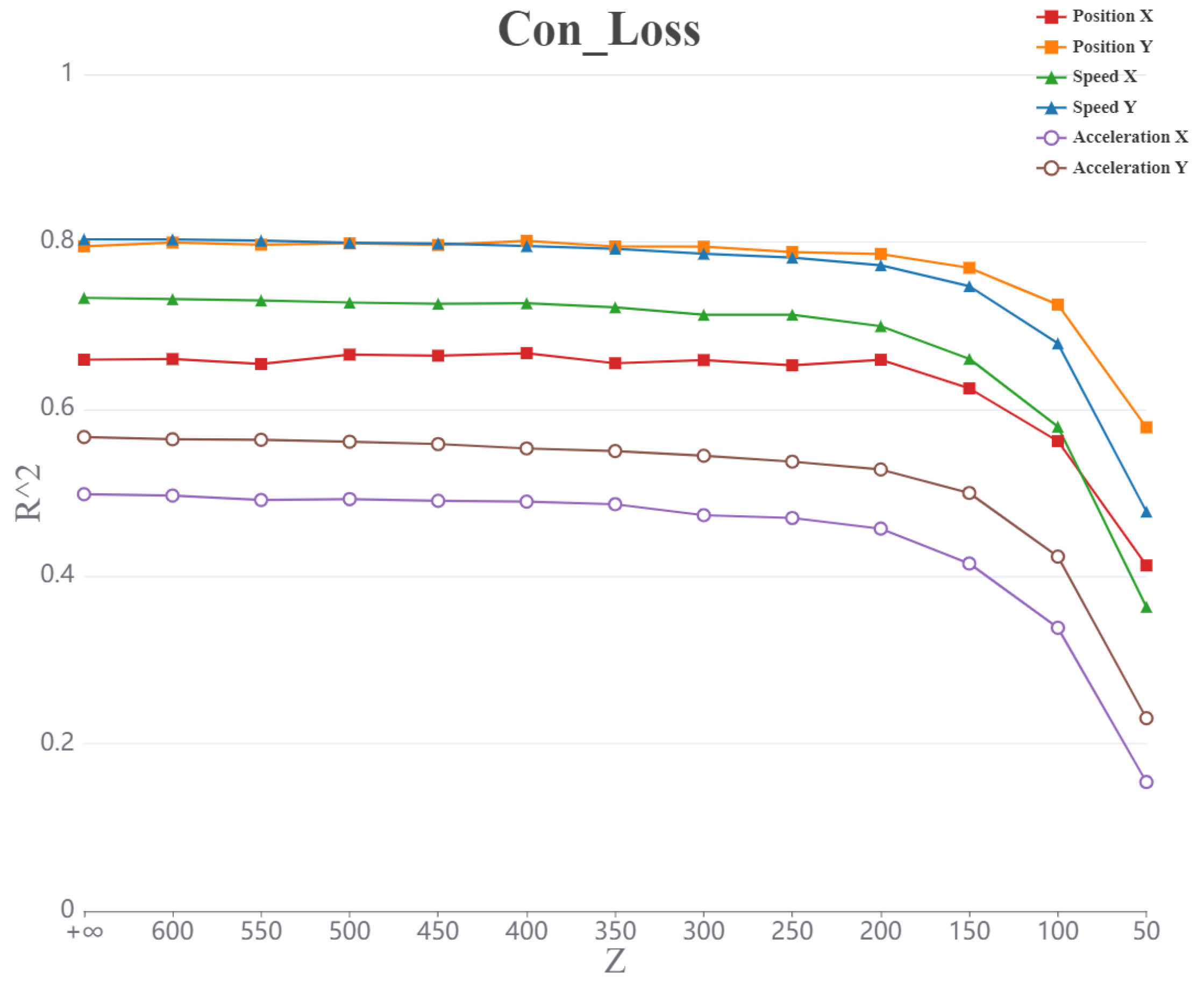
Figure 8.
(a)Curve of values representing position (X, Y) as a function of increasing packet loss rate for different packet loss models.(b)Curve of values representing speed (X, Y) as a function of increasing packet loss rate for different packet loss models.(c)Curve of values representing acceleration (X, Y) as a function of increasing packet loss rate for different packet loss models.

Figure 9.
Illustrative reconstructions. Reconstructions of a typical reach (dotted black lines) using the refh position decoders, with the burst loss model. Only sagittal ( x ) kinematics (position) are shown since the lateral (y) reconstructions are similar. These reconstructions correspond to the test data for session Indy2016040702.
Disclaimer/Publisher’s Note: The statements, opinions and data contained in all publications are solely those of the individual author(s) and contributor(s) and not of MDPI and/or the editor(s). MDPI and/or the editor(s) disclaim responsibility for any injury to people or property resulting from any ideas, methods, instructions or products referred to in the content. |
© 2024 by the authors. Licensee MDPI, Basel, Switzerland. This article is an open access article distributed under the terms and conditions of the Creative Commons Attribution (CC BY) license (http://creativecommons.org/licenses/by/4.0/).
Copyright: This open access article is published under a Creative Commons CC BY 4.0 license, which permit the free download, distribution, and reuse, provided that the author and preprint are cited in any reuse.
MDPI Initiatives
Important Links
© 2024 MDPI (Basel, Switzerland) unless otherwise stated


