1. Introduction
Apple proliferation (AP) is one of the most economically important diseases of apple and is widespread in Europe. It reduces fruit size and quality which leads to a total yield loss of infected trees [
1]. The causal agent, the phloem-limited cell wall-less bacterium ‘
Candidatus Phytoplasma mali’ is therefore treated as non-regulated quarantine pest. It is efficiently transmitted by the psyllids
Cacopsylla picta and
Cacopsylla melanoneura [
2]. As there are no curative treatments against this disease, preventive measures as uprooting of infected trees and vector control are the only means so far to prevent further spread of the disease. E.g. in some regions of Italy farmers are made responsible to uproot infected trees by law [
3]. For the implementation of these measures, the identification of infected trees on a large scale is of great importance. Although AP induces typical symptoms like witches’ brooms and enlarged stipules [
1], these are often difficult to diagnose. Confirmation by molecular means is often required. Large scale monitoring by experts is time-consuming and expensive.
In order to overcome these limitations, we studied the possibility to detect AP by optical measurements. For this, a secondary symptom of AP, the reddening of infected trees in early autumn, was used. We could show in a parallel study based on the monitoring of more than 20,000 trees that premature leaf reddening is a highly reliable symptom of AP [
4]. It was observed in almost 100% of trees showing specific AP symptoms. In this combination, it has already been regarded as typical indication for an AP infection [
3,
5]. Depending on the year of monitoring, ‘
Ca. P. mali’ was also detected by PCR in 71–97% of trees that showed reddening without any other AP symptom. Öttl et al. report a correlation of 86% to AP-infection in South Tyrol [
6]. AP-related leaf reddening is induced by cold night and warm day temperatures in September [
4]. It is the consequence of chlorophyll breakdown induced by the phytoplasma infection [
7]. Its potential for spectral detection of AP has already been evaluated by Barthel et al. who found differences between infected and healthy grounded leaf samples analyzed by near-infrared spectroscopy [
8]. However, this is a destructive approach which is still lab-based and labor-intensive. Therefore, Barthel et al. tested a sensor-based method to distinguish AP-infected from healthy leaves in the field with a portable spectroradiometer. By analyzing leaf hyperspectral signatures between 350 and 2500 nm, they were able to identify relevant wavelengths for AP infection [
9]. However, this work was conducted only in one infected orchard with one cultivar. It remained uncertain whether the results can be transferred to other orchards with different cultivars and different management strategies.
Biochemical and biophysical modifications induced by pathogens in their host plant have been increasingly used for the development of sensor-based non-invasive detection methods. As phytoplasmas induce chlorophyll breakdown also in many other plant species, this has already been used to detect phytoplasmas infecting grapevine. Al-Saddik et al. developed spectral disease indices [
10] for the detection of the quarantine pest Flavescence dorée which could be used for field detection methods [
11]. In Germany, hyperspectral imaging (400–2500 nm) was successfully applied to identify two other distinct grapevine yellows diseases: bois noir and Palatinate grapevine yellows [
12].
To gain insights on the appearance of infected trees and to overcome existing limitations, we studied the spectral signatures of infected and healthy leaves with hyperspectral imaging under laboratory conditions. The development of a processing pipeline und utilization of machine learning algorithms aim to derive information about the relevance of certain spectral bands with respect to AP symptoms. This information can then be used to support on-site phenotyping by adapting optical remote sensing technology to the special requirements of AP detection.
2. Materials and Methods
2.1. Plant Material
Two types of material were used for spectral imaging studies: 1) leaves of greenhouse grown
ex vitro plants infected with a defined strain of ‘
Ca. P. mali’ and 2) freshly field collected leaves of AP-symptomatic trees in apple orchards.
Ex vitro plants of
M. x
domestica cv. Golden delicious were infected with ‘
Ca. P. mali’ strain PM28 originally transmitted by
Cacopsylla picta in previous transmission trials [
13] and since maintained in micropropagated plants. Healthy plants of cv. Golden delicious served as controls. The plants were part of different experiments to induce AP-related reddening under standardized conditions [
4]. Each experiment consisted of 3 infected and 3 healthy plants which were maintained under autumn climatic conditions (12h cold night at about 5°C/12h warm day temperatures at about 20°C) and a second set of 3 infected and 3 healthy plants which were maintained in parallel under constant warm temperatures (12h at about 18°C at night/12h at about 22°C at day). At the end of the experiment, 10 leaves per plant were analyzed by hyperspectral and molecular means. We refer to this experiment as AP-induction by temperature profile (AP-ITP) experiment. Three datasets were analyzed in this study: AP-ITP-1 (induction period 5 September–20 September 2019), AP-ITP-2 (induction period 24 September-9 October 2019) and AP-ITP-3 (induction period 3 September-21 September 2019).
To investigate the variability of leaf related AP symptoms under natural field conditions, we collected numerous samples from production orchards. The focus was laid on older apple orchards to raise chances to find a high number of AP-infected trees. The orchards were monitored for AP-specific symptoms like witches’ brooms and enlarged stipules as well as for leaf reddening [
4]. In 2019, samples from reddening trees were taken in the first half of October. In 2020, samples were taken in the second half of September. Non-symptomatic trees served as controls. All sampled trees were tested by PCR for phytoplasma infection.
Table 1 gives an overview of the analyzed orchards and cultivars. In total, 21 different cultivars from 13 different orchards were analyzed. We refer to this experiment as AP-field test samples (AP-FTS).
2.2. Data Collection
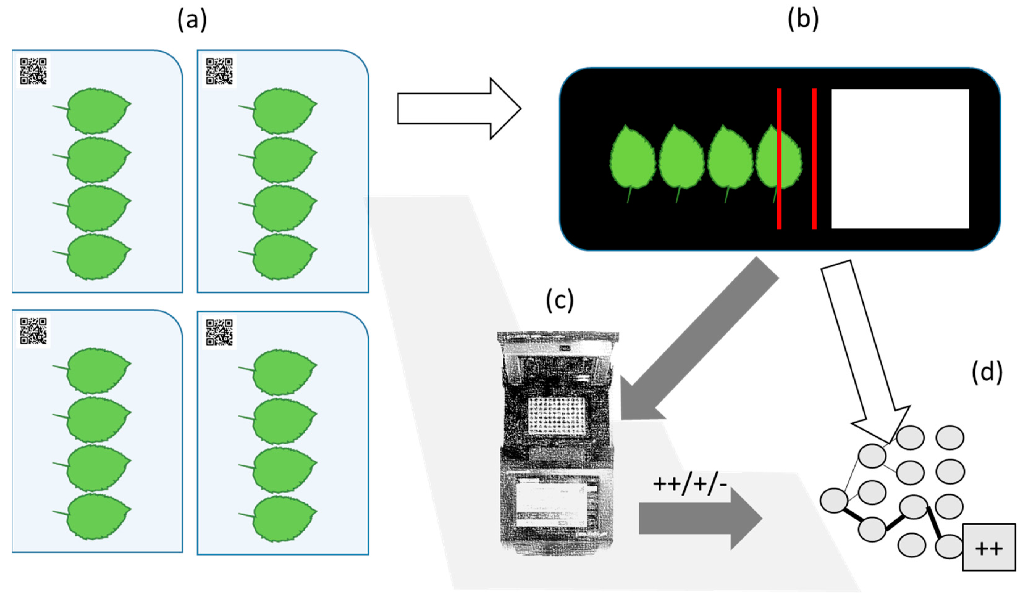
Following the idea to implement a non-destructive optical assessment of the disease and its symptoms, data collection consists of spectral imaging of the collected plant material. Carried out under laboratory conditions this approach yields the highest potential to identify relevant wavelength bands at leaf scale as well as a baseline for subsequent performance evaluation of outdoor measurements at canopy scale. The collected spectral data has to undergo several steps of preprocessing. To obtain predictions of disease symptoms, machine learning techniques are applied. Predictions are compared against ground truth data from molecular analysis of the collected leaves. The imaging approach is shown in
Figure 1 and described in the following sections.
2.3. Spectral Imaging
A hyperspectral dual camera setup was used throughout the experiments. Depending on the experiment, one of two camera setups was used.
For the AP-ITP-1 experiment, a fixed dual camera installation at the Julius Kühn-Institut located at Siebeldingen, Germany, was used. It consists of a Norsk Elektro Optikk (NEO) VNIR-1800 and a NEO SWIR-384 hyperspectral imager. Both cameras are push broom sensors and record single lines of spectral image data at a given frequency. Therefore, the imaging process requires either moving of the samples or moving of the camera system. Here, a moving table is used. In
Figure 1 the dual line scanner setup is represented by the two symbolic scanlines in step (b).
For the AP-FTS experiment, a mobile dual camera installation at the RLP AgroScience institute in Neustadt was used. It consists of a NEO VNIR-1600 and a NEO SWIR-320m-e hyperspectral imager. Leaf assays of 10 leaves per plant for the AP-ITP (AP-ITP-2, AP-ITP-3) and 4 leaves of each tree for the AP-FTS experiments have been hyperspectrally recorded for subsequent analysis. Initial preprocessing of the acquired data consists of (1) radiometric correction based on manufacturer calibration data to obtain at-sensor radiance values and (2) normalization with respect to a calibrated white reference plate to obtain at-surface reflectance data.
Table 2 lists the specifications of the different cameras. A detailed assessment of the imaging quality and additional key parameters can be found in [
14]. Its application is not bound to a laboratory environment [
15].
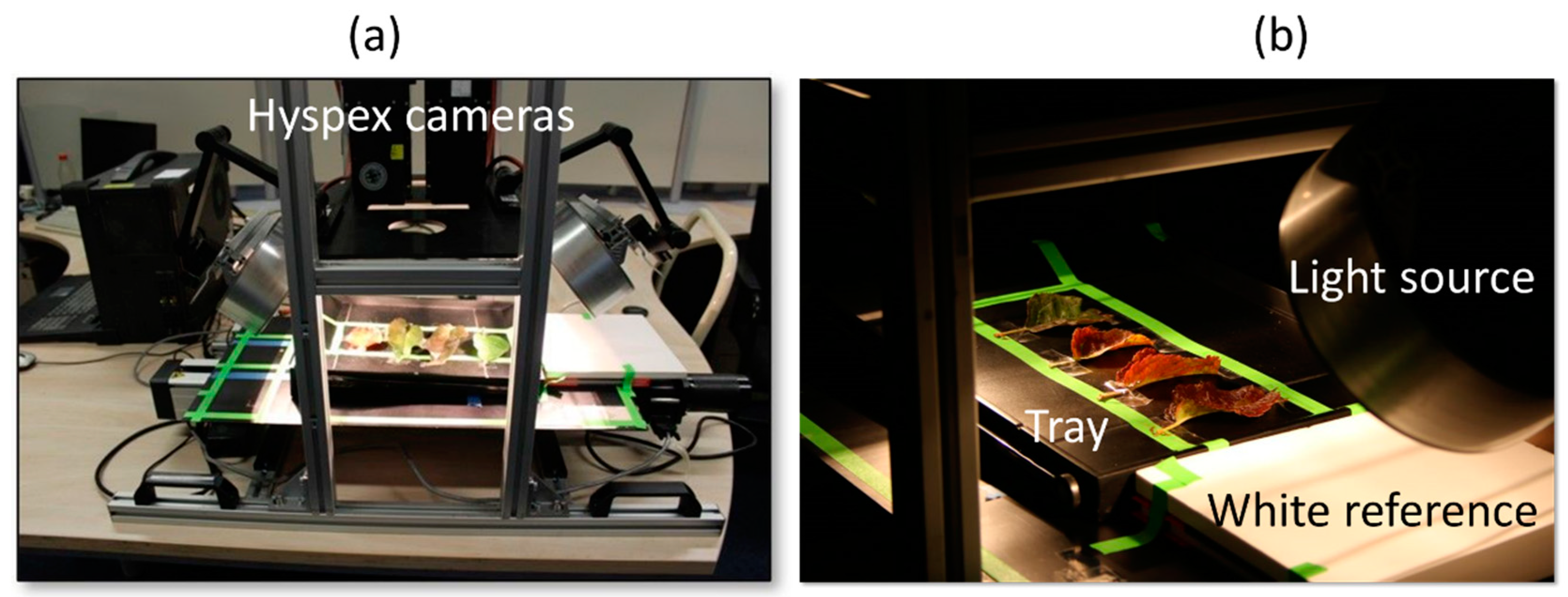
Figure 2 shows the rack-mounted camera setup at RLP AgroScience (VNIR 1600, SWIR 320m-e).
The integration time for each scanline is individually adjusted for the recording of each experiment. Especially, the mobile rack solution used at RLP AgroScience requires this adjustment due to slightly varying positions of the light sources. The recording software Hyspex Ground stores the hyperspectral images in ENVI format. Each scan consists of two ENVI images, one for each camera. The software Hyspex Rad is then used to obtain at-sensor radiance using a camera specific calibration profile prerecorded at the manufacturer’s laboratory using a light measurement integration sphere.
2.4. Image Processing
Figure 3 illustrates the measured hyperspectral image data. We implemented two different processing chains for data analysis. First, a highly automated processing for fast assessment of the data for analyzing the AP-FTS data. Second, an interactive processing chain to achieve a precise segmentation by revision of automated segmentation by human experts to obtain the highest possible accuracy for subsequent steps of the analysis. This processing chain is used to analyze AP-ITP data.
2.4.1. Automated Processing
For testing close to real-world conditions, we developed an image processing pipeline using the C++ programming language and the OpenCV computer vision library. Based on [
16], the pipeline extracts spectral data as well as derived spatial-spectral image features for the subsequent machine learning based data analysis.
First, the position and extents of the white reference panel must be located within the image. Its spectral appearance depends on the camera settings like framerate and integration time as well as on the intensity and spectral characteristics of the used light source. Therefore, an interactive approach ensures that the algorithm can easily be adapted to changing conditions. Within a single channel preview image (obtained as mean intensity of all bands) a scaling value must be selected via a slider control to obtain a visually good separation between the reference plate and the remaining image. The second interactive step consists of selecting a threshold for binarization of the image to obtain a good segmentation. Immediate feedback is provided for each step by applying the scaling factor and the threshold online. This interactive procedure can be repeated for the next images until good values are found. Given stable lighting condition throughout the experiment, well-suited parameters can be found within a few steps. Next, the tool can enter an automatic mode to process the complete dataset using the selected parameters.
Next, a sample of spectra at random locations of an image (N=1000) on a random subset of the hyperspectral images (N=15) is drawn. The reflectance of the white reference panel is used to normalize all spectra. Then, dimensionality of the feature space is reduced by applying a principal component analysis (PCA) [
17]. A dynamically selected number of principal components is used. Dynamical selection is implemented such that at least 98 % of the variance within the spectral dataset must be represented by the subset of principal components. Unsupervised clustering with multiple iterations of the k-means algorithm [
18] is used to determine an optimal choice of k. The criterion for the choice of k is minimization of a compactness measure, where the average Euclidian distance between each sample and the center of the corresponding cluster must be determined for different choices of k. For each of the k selected clusters, small grayscale preview images of randomly selected samples are extracted, arranged and presented to the user as a preview of the cluster. The relatively simple task to judge, whether the cluster represents image foreground (e.g. leaves) or background (e.g. white reference plate, metal background) is solved interactively. This constitutes a general pipeline for hyperspectral image analysis where domain knowledge about objects of interests is acquired by asking the user the simple question, whether the set of images represents foreground or background. Based on the acquired reference data, a Random Forest [
19] segmentation model is trained and applied to all hyperspectral images afterwards.
After image segmentation into leaf area and image background, individual objects are detected within the leaf area class. A comma separated value (CSV) file is generated, which lists all detected objects within all the images. Unique object identifiers are generated according to an enumeration scheme. Next, the reference data is added to the generated CSV file. In our experiments, either discrete class information (infected or healthy based on PCR) or continuous reference data (count of phytoplasma per volume from qPCR results) is added as separate columns to the CSV file.
Next, a predefined number of spectra is extracted for each object. Again, spectra are stored in CSV format and the given reference data is automatically appended to each spectral sample. The CSV files constitute the datasets used for further processing and data analysis. Derived classification or regression models can then be applied to either CSV stored data or the original hyperspectral images.
2.4.2. Interactive Processing
For precise interactive preprocessing a similar approach using a MATLAB-based framework called HawkSpex
® Flow is used that has been successfully used in several studies [
12,
20,
21]. Each image of detected leaves is manually validated and automatically obtained segmentation results are improved using a manual labeling tool. Instead of k-means clustering for the initial image segmentation, a Growing Neural Gas [
22] is used.
2.5. Feature Extraction and Machine Learning
In order to compare different classification algorithms, different datasets are prepared representing different subsets of the conducted experiments and different feature spaces.
Section 2.5.1 describes the used features and
Section 2.5.2 is devoted to our choice of ML algorithms.
2.5.1. Feature Extraction
Prior to evaluation of machine learning, the hyperspectral data is transformed into different feature spaces. In this study, the following feature spaces are investigated:
Spectral reflectance
Normalized spectral reflectance
Dimensionality reduced spectral data
Spatial-spectral data
Selected spectral indices
Spectral reflectance data consists of the reflectance values for each wavelength band of the hyperspectral image. At-sensor radiance is transformed into reflectance values by division of the radiance value at each pixel by the radiance value measure at the location of the white reference panel. In order to obtain spectral reflectance, the position of the white reference panel in the image must be provided either manually or automatically. Using spectral reflectance data as feature vector for machine learning enhances the interpretability of the results. Each dimension of the feature space corresponds to a certain wavelength of light and variable importance measures can be used to determine and understand the physical interaction of the light with the measured materials.
Normalized spectral reflectance is obtained by normalizing each feature vector by its Euclidian norm (L2 norm), which corresponds to the length of the vector. After normalization all feature vectors have equal length of 1. Using normalized spectral reflectance is beneficial if the total amount of reflected light differs due to shadows or the bidirectional reflectance distribution function (BRDF) of the material. Again, the wavelength bands constitute the dimensions of the feature space. Therefore, importance measures can also be derived and easily interpreted. However, information about the fraction of reflected light in certain bands is lost when different feature vectors are compared and interpretation becomes more difficult.
Dimensionality reduced spectral data is based on PCA. It projects the dataset into a low dimensional feature space, which preserves most of the variability of the original dataset. Each dimension of the novel feature space is a linear combination of all original dimensions. It is an orthogonal transform which ensures linear independence of the principal components (base vectors of the new feature space). As the novel features are linear combination of the original features, it is more difficult to interpret the feature values. The PCA outcome depends on the used dataset and the transformation matrices might change dramatically, if new samples are integrated into the dataset.
Spatial-spectral data integrates the spectral information and data from neighboring pixels. Different approaches exist. In our study, we apply linear discriminant analysis (LDA) to preserve class-specific spectral information. The high dimensional feature space of spectral data is transformed into a low dimensional feature space, where each dimension is an optimized feature with respect to separation of one of the classes. Each new dimension is a linear combination of all original dimensions and therefore important information of the spectral data is preserved in the low dimensional feature space. Spatial information is integrated by calculating different statistical measures for different image blocks centered around the image position of the feature vector. Here, we use three different statistical measures (mean, standard deviation, homogeneity), the first three components of the LDA, and 25 different block sizes (4x4 to 100x100 pixels). This results in a 225-dimensional feature spaces. Using spatial-spectral features intends to integrate information about the spatial distribution and variation of object reflectance into the pixelwise decisions of a classifier. Therefore, it adds additional robustness to the decision making. However, as the information from the neighborhood gets more important, small regions of interest might be more difficult to detect by a classifier.
Spectral indices aim to reduce dimensionality of spectral data and to allow for a high interpretability of the feature values. Typically, a spectral index comprises only a few spectral bands to calculate a problem specific measure. Most spectral indices originate from the field of remote sensing and address properties of vegetation, soil, water bodies, and other surfaces. Here, we focus on selected spectral indices only, namely NDVI, PRI, CCI, and GLI. Selection is based on the ability to detect various plant stresses (NDVI), vegetation health (PRI), and chlorophyll content (CCI, GLI). Definitions and references of spectral indices are provided in
Table 3. Using spectral indices provides a highly interpretable feature space but limits the information to only a few bands. This yields the chance to miss important features when applied to new classification problems.
2.5.2. Machine LEARNING
For evaluation of different machine learning approaches MathWorks Matlab (version 2024a) is used. Evaluation uses two different approaches:
experiments using own implementations of ML algorithms, and
experiments using the suite of provided ML algorithms.
The first approach uses a self-developed framework that has been described in
Section 2.4.2 for interactive preprocessing. The second approach uses the integrated Matlab apps Classification Learner and Regression Learner (Statistics and Machine Learning Toolbox)
Both kinds of experiments aim to
identify most relevant wavelength bands for detection of apple proliferation
identify best feature space – classifier combinations to solve the detection problem
better understand options and limitations of automated diagnosis of the disease
propose an approach for implementation of disease detection
From the set of available methods, the following ML algorithms have been selected for investigation:
Decision trees with different levels of pruning
Ensemble methods based upon decision trees
Support vector machines with different kernels
Neural Networks with different topologies
To compare results, n-fold cross validation (n=10) is used in an integrated training and testing approach. Stratified datasets are used and mean classification accuracy, confusion matrices and ROC-curves are used as means to evaluate classification performance. Root mean square error (RMSE) is used as a measure to compare different regression methods for prediction of disease levels. Based on the results of the experiments, the Random Forest classifier as a fast to train as well as general-purpose ensemble classification method has been implemented into the automated processing pipeline described in
Section 2.4.1. for analyzing the AP-FTS experiment.
2.6. PCR Analysis
For the AP-ITP experiment each leaf was tested individually for phytoplasma infection. For the AP-FTS experiment the entire trees was tested. Total nucleic acids were extracted either from leaf petioles (AP-ITP) or from phloem preparations of branches (AP-FTS) according to [
13] using a CTAB-based protocol. For phytoplasma detection European fruit tree phytoplasma-specific primers fO1/rO1 were used as published in [
28]. Aliquots of each PCR-product were analyzed by agarose gel electrophoresis.
The phytoplasma titer was analyzed in the AP-ITP experiment in the individual leaves by quantitative PCR as described in [
4]. Specific primers AP3/AP4 were used for absolute quantification with the standard curve method according to Jarausch et al. [
29]. These data were normalized with the absolute quantification of an apple single copy gene according to Liebenberg [
30]. Phytoplasma concentration in each leaf was thus expressed as phytoplasma copy per plant cell.
3. Results
In this section, the results of different experiments with the AP-ITP and AP-FTS datasets are provided. First, detection of AP infections with regression methods as automation of the lab-based PCR approach is presented for the AP-ITP experiment. Second, results of binary classification (infected vs. healthy) for the AP-ITP experiment are presented. This includes assessment of the relevance of spectral bands for solving the classification problem. Third, existing spectral indices are investigated as a means to provide reliable disease detection. Fourth, performance of different ML algorithms for disease detection using spectral data from the complex AP-FTS dataset is presented. Finally, possible improvements by using spatial-spectral features instead of spectral data are reported.
3.1. Regression of qPCR Values to Estimate Infection Levels (AP-ITP-1)
Infection with AP was validated with qPCR for the experiment AP-ITP-1. Therefore, we used this dataset to evaluate the potential of different regression algorithms to predict the qPCR value.
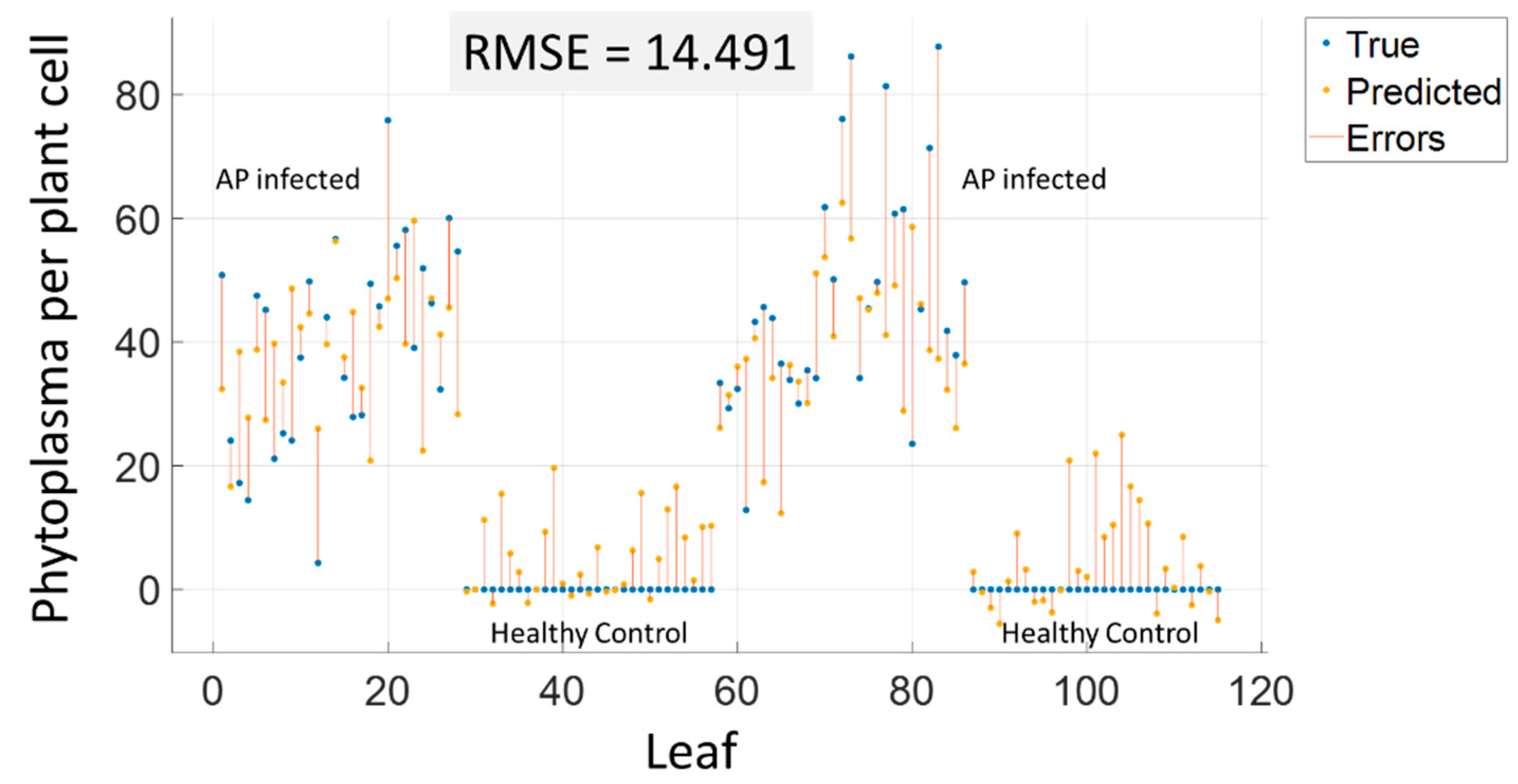
Figure 4 shows the validation plot of the best performing method.
Table 4 lists the results of different regression algorithms. The best RMSE, as presented in
Figure 4, was achieved by limiting the number of input features to 20 most important wavelength bands using RReliefF algorithm [
31], to further reduce dimensionality by PCA to 10 features, and by using Gaussian Process Regression. For all other regression algorithms, the table reports the results of similar feature reduction as well as the individually best performing approach of each alternative approach. For Gaussian process regression results within other feature spaces and for different feature selection algorithms are reported to provide a good summary of the prediction quality.
The response of the regression method was obtained by 10-fold cross-validation. The results indicate that prediction of medium concentrations is better than prediction of high concentrations and detection of healthy leaves. Based on the obtained RMSE value, a detection threshold can be defined to minimize false detections. In addition, classification of the symptoms can be combined with the regression method in a hierarchical approach to improve the results.
3.2. Classification of Spectral Data (AP-ITP-2, AP-ITP-3)
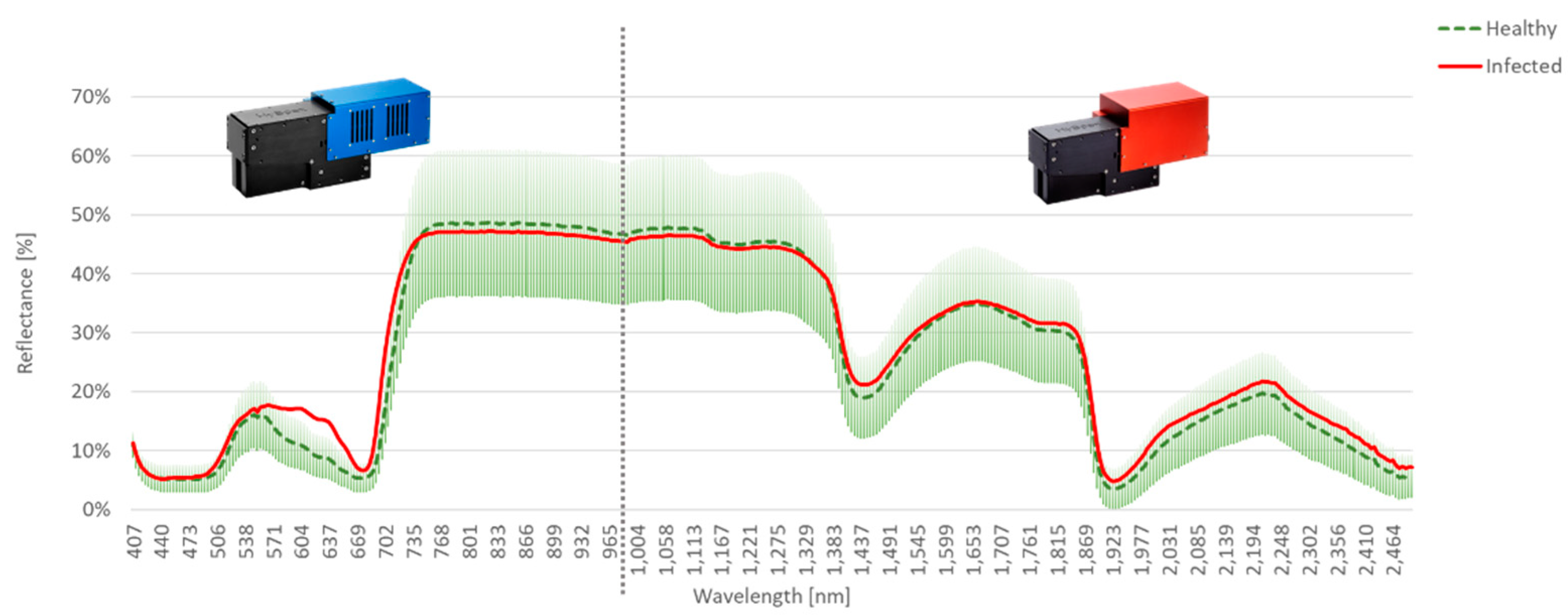
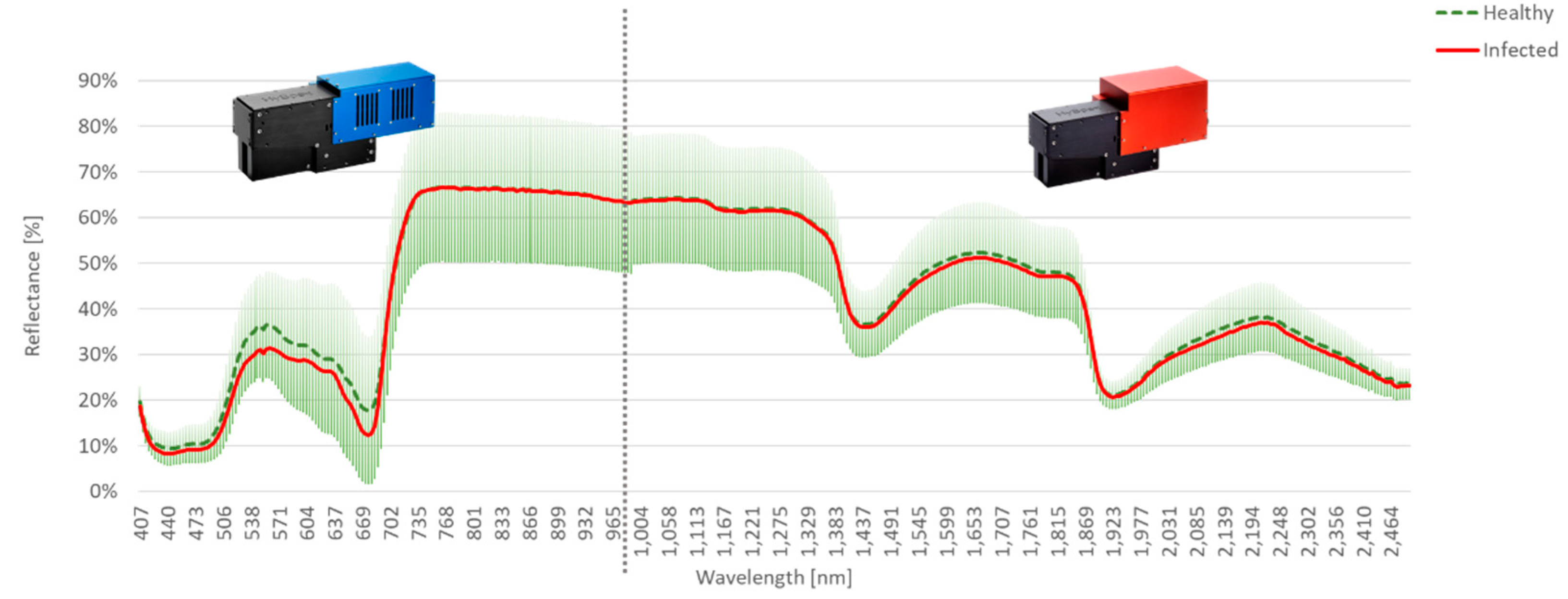
The comparison of the measured spectral data for AP-ITP-2 is shown in
Figure 5. For the healthy leaves the standard deviation of reflectance is plotted in addition to the average spectrum. The mean spectrum of infected leaves clearly shows a difference between the two classes in the spectral bands between the so-called green peak (~550 nm) and the beginning of the so-called red edge region (~700 nm).
In contrast to the visible and near infrared bands, no clear difference is visible in the shortwave infrared, given the high standard deviation within the pixels of the healthy leaves.
Figure 6 shows the observed mean spectra of the experiment AP-ITP-3. Again, the differences in the mean spectra concentrate in the visible region between the green peak and the start of the red edge. However, differences in the reflection of green light are observable in lower bands compared to AP-ITP-2. Also, the differences in the shortwave infrared region and the water absorption bands are visually less significant.
Diagrams in
Figure 5 and
Figure 6 provide a visual cue, which bands are of special interest for an automated diagnosis of apple proliferation disease by hyperspectral remote sensing. The presence of a high standard deviation for the measured reflectance per pixel within these bands highlights the need for more sophisticated classification approaches.
Table 5 contains the confusion matrix for the classification of VNIR data using an Auto-ML-approach. Here, the 10-fold cross-validation results of the best performing ML-algorithm are provided. The used dataset is balanced with the same number of spectra of infected and healthy leaves. Spectra are randomly selected from the full dataset.
Table 6 contains the results of classification of SWIR data.
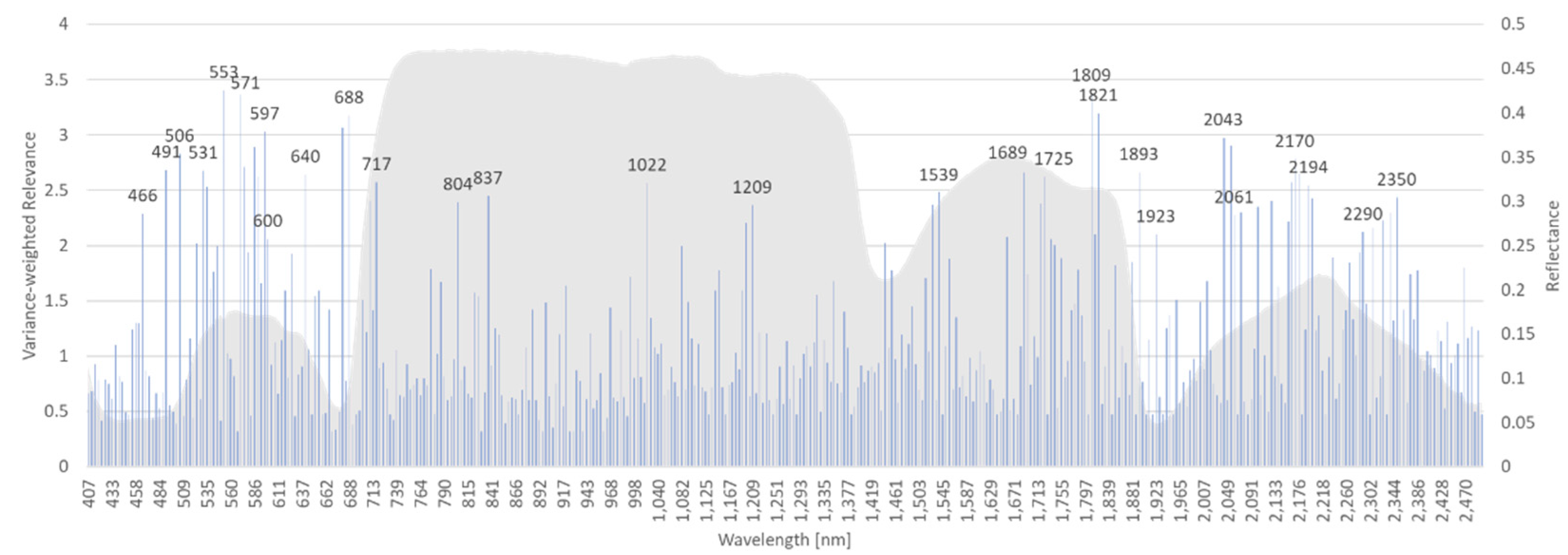
The rRBF classifier yields a weight vector for the input features as an additional result of model training. This can be interpreted as the relevance of input features and as a starting point for reduction of dimensionality and model complexity. As 10-fold cross-validation results in 10 different models, also the variance of the weights is obtained. It is used to weight the mean relevance of each band. Bands with high variance of relevance in 10-fold cross-validation get a lower weight and vice versa. Relevance values for AP-ITP-2 are shown in
Figure 7.
In a similar way, dataset AP-ITP-3 has been analyzed.
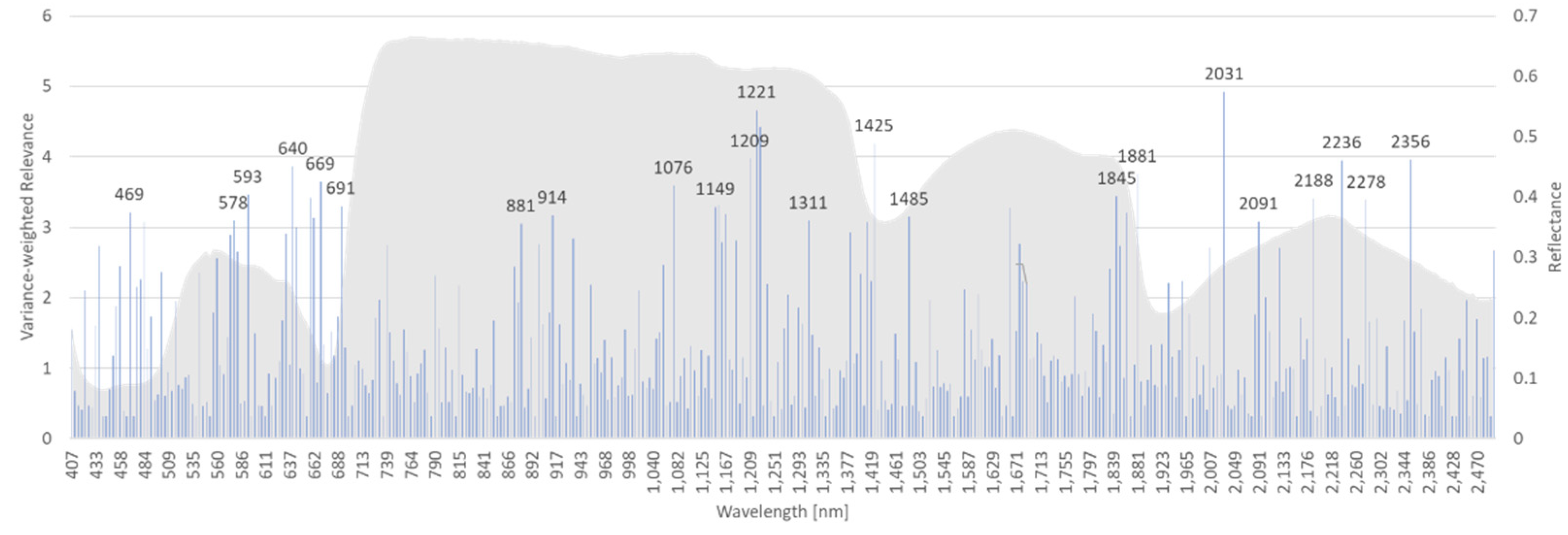
Figure 8 shows the variance weighted relevance of individual bands in the decision process of the rRBF classifier.
For both experiments (AP-ITP-2, AP-ITP-3) the results indicate the importance of the complete spectral information to achieve the classification accuracy of 0.971 in cross-validation. Also, the high number of relevant bands indicate the complexity of the detection problem. The insights, that the machine learning approach provides by the relevance measure, help to judge on the importance of the visible differences in the mean spectra (
Figure 5 and
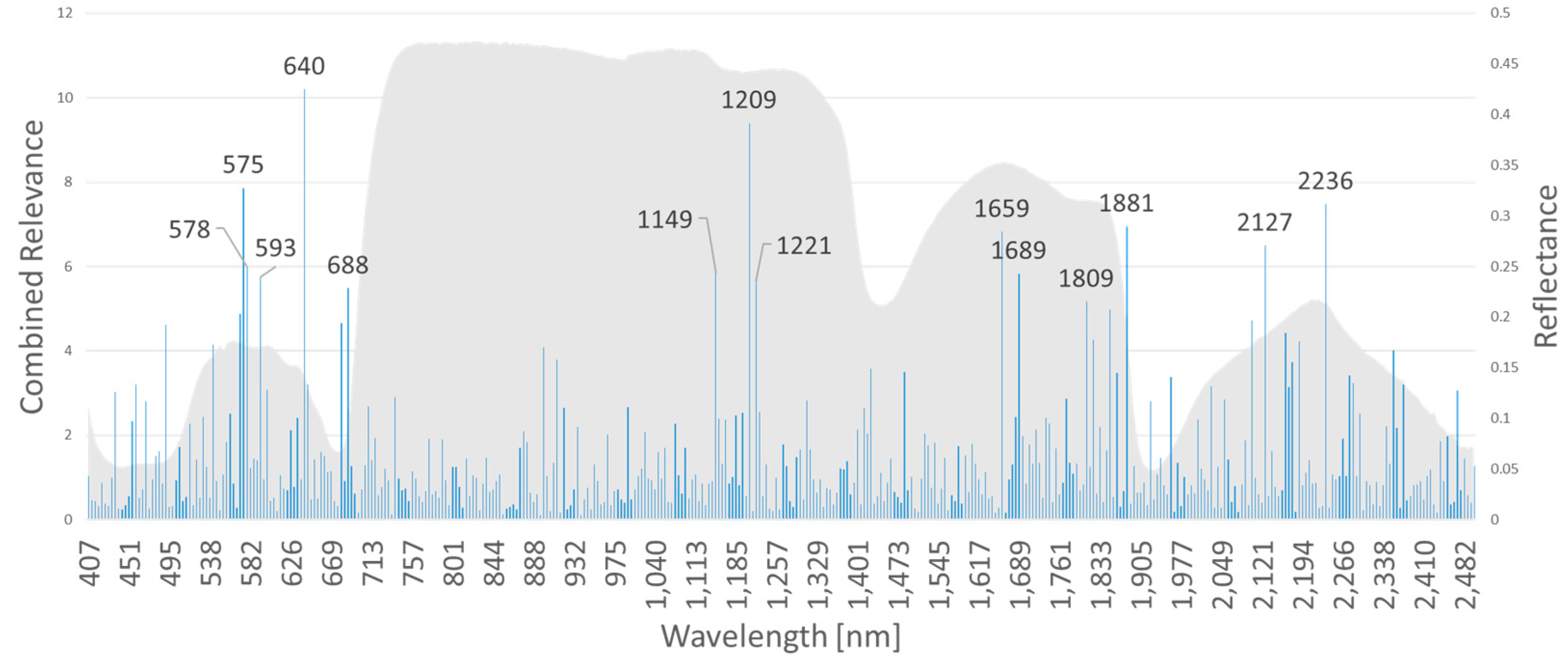
Figure 6). By multiplying the band specific relevance measures of AP-ITP-2 and AP-ITP-3, bands of general interest and relevance for detection of an AP infection in both experiments can be emphasized.
Figure 9 shows the results. Five bands in the visible part of the electromagnetic spectrum and nine bands in the NIR and SWIR part are of special interest. Here, a threshold of 60 percent of the maximum relevance measure (located at 640 nm band) was used to discriminate between relevant and less relevant bands.
3.3. Spectral Indices
Spectral indices are a means for dimensionality reduction in spectral data analysis by preserving a high level of information with respect to common traits in monitoring the vegetation and the environment.
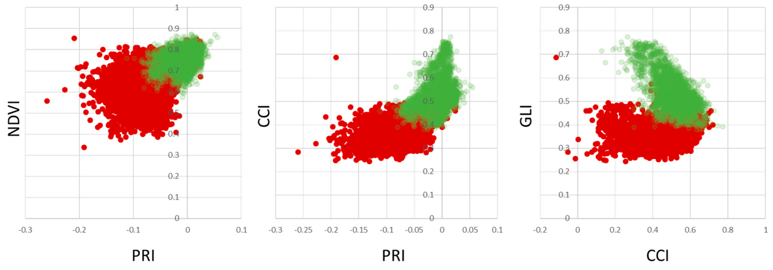
Figure 10 shows scatterplots of healthy vs. infected leaves per pixel. The overlap of the points clouds within the scatter plots indicate, that healthy plant material within infected leaf tissue limits the ability to discriminate between healthy and infected leaves. However, the distribution of pixels belonging to healthy trees clearly indicates a unique distribution within the three feature spaces shown. As PRI, NDVI, CCI and GLI are commonly used vegetation indices to detect plant stresses, chlorophyll concentration and senescence, the results provide support to their potential application to detect apple proliferation disease.
To overcome the limitations of separability, different measures that can easily be implemented into automated disease detection algorithms have been investigated.
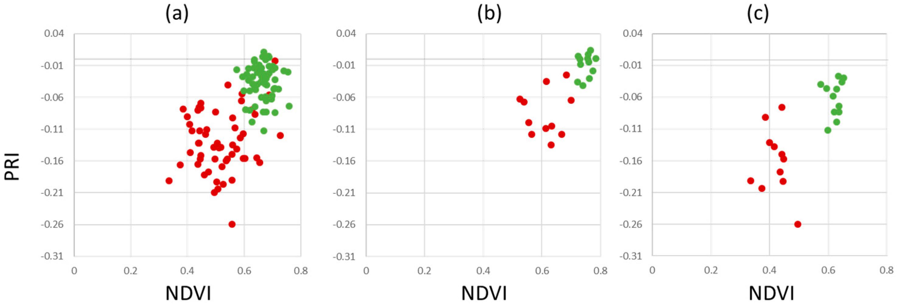
Figure 11 shows the results for our dataset AP-ITP-2. Using the minimum NDVI value per tree (condition c, an assay of 5 leaves per tree has been used) provides a reliable separation between healthy and infected trees. Using the average NDVI value in combination with average PRI (condition b) already provides clear distinction between classes and is assumed to be more robust to outliers. However, if diagnosis is based on single leaves, false classifications still persist (condition a).
Validation of the findings from AP-ITP-2 with a different experiment (AP-ITP-3) yield different results with respect to the value distributions and separability of healthy and infected leaf pixels.
Figure 12 shows PRI, NDVI, CCI and GLI scatter plots.
The aggregation of the pixelwise measurements using mean values per leaf as well as per tree improve performance (see
Figure 13). However, using the minimum value for the spectral indices NDVI and PRI does not improve the results (
Figure 13(c)).
3.4. Apple Proliferation Detection Pipeline (AP-FTS)
The next step is the integration of classification models into a highly automated AP detection pipeline. Therefore, different machine learning approaches are investigated for their performance with an automated feature extraction (without manual revision of the extracted data). The spectral data, that constitutes the training set, is obtained by random sampling from the hyperspectral images. First, it is normalized by L2-norm and then it is used as input to a suite of classification algorithms for direct comparison of the classifier performance. Stratified sampling was used within each hyperspectral image. Because trees with apple proliferation and healthy trees are not equally represented within the images, stratification is applied to provide an equal number of spectra for the 2 classes.
Table 7 summarizes the classification performance of the selected ML algorithms. For the 2019 measurements, the Hyspex SWIR camera in combination with SVM classifier provided best results. For the 2020 measurements, again the SWIR camera yields better results, but in combination with the Random Forest classifier. The results of the Hyspex VNIR camera are slightly less reliable than SWIR data for both years. Either, ensemble methods or SVM classifiers yield the best results.
Figure 14 shows confusion matrices for the best performing variants of each group of methods in
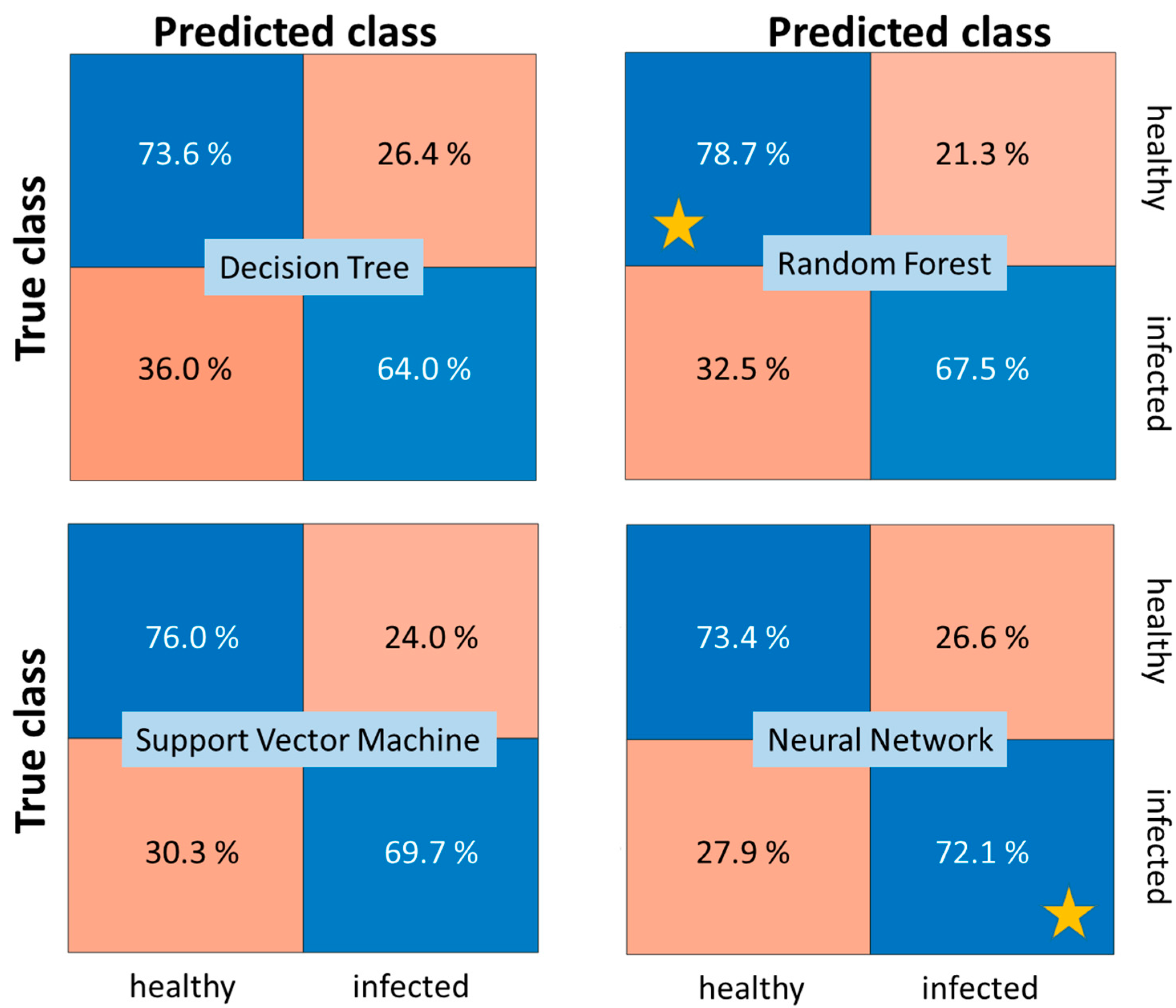
Table 7 to gain more insights into the classification performance and differences among the classification approaches. While the Random Forest classifier yields the best overall performance, it also minimizes the number of false detections of an infection compared to all other methods. However, the MLP neural network classifier is capable to detect more of the true infections and nearly matches the overall performance of the Random Forest.
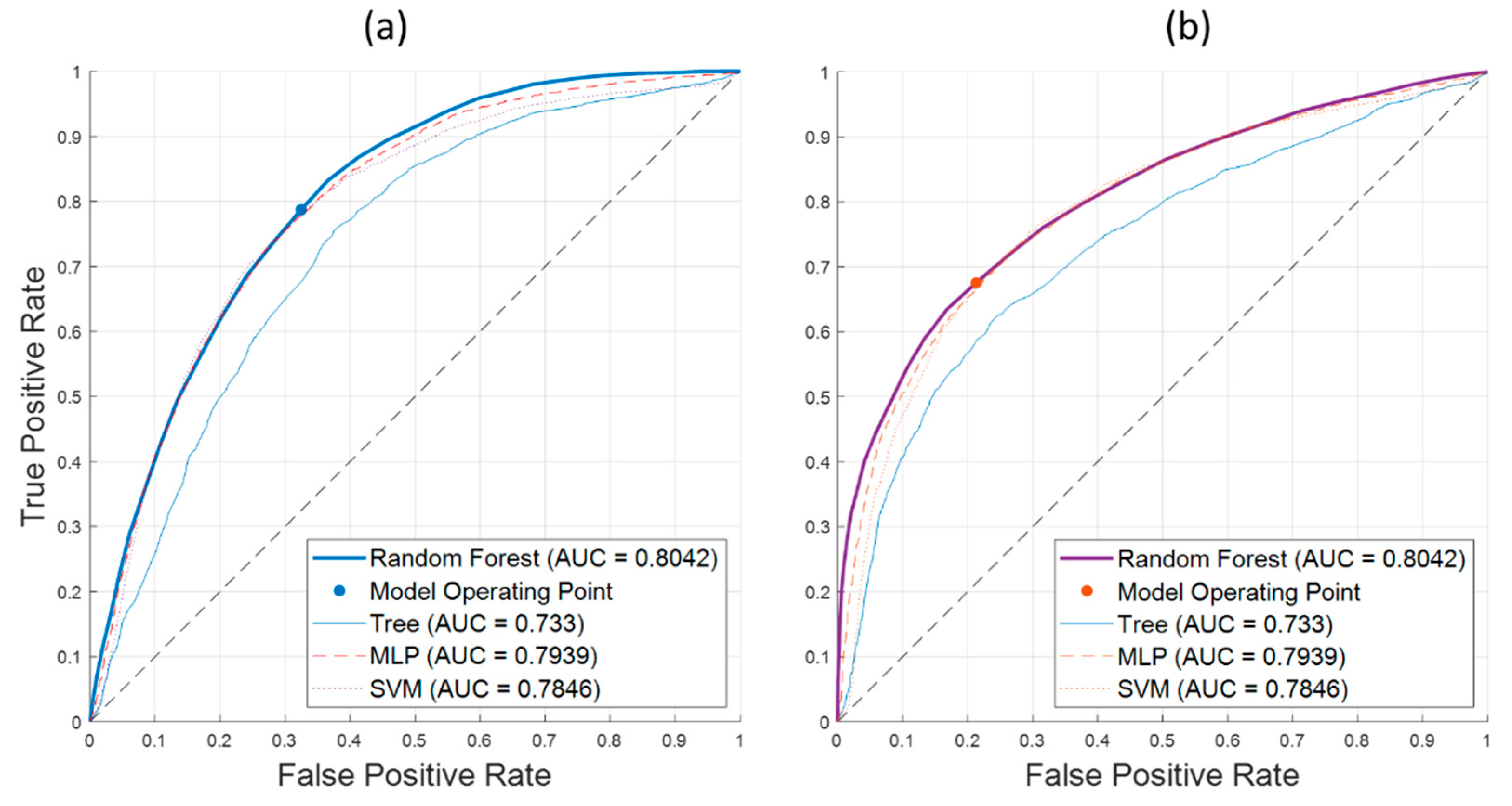
Figure 15 shows ROC-curves for (a) the detection of spectra from healthy leaf tissue and (b) the detection of spectra from leaf tissue of AP infected trees. Again, the Random Forest classifier shows its superior performance over the full range of possible operating points. This corresponds to the AUC measure of 0.8042. The operating points correspond to equal classification costs and the accuracy values in
Table 7.
Given, that the Random Forest classifier yields the best performance in the SWIR 2020 dataset and overall good ranking among the other datasets (2nd rank on all datasets), it was chosen for integration into the automated detection pipeline.
As a consequence, the application of the Random Forest classifier yields pixel-wise classification results for all available AP-FTS images from years 2019 and 2020. As the degree of reddening as well as affected leaf surface differ between different varieties and the date of sample collection, a health index is calculated from the pixel-wise decisions. The health index is the fraction of healthy leaf surface based on pixelwise decision of the Random Forest classifier.
Figure 16 compares the performance using measurements with Hyspex VNIR only, Hyspex SWIR only, and both cameras.
Postprocessing is applied to further improve the results. It consists of a morphological operation (dilation with 5x5 rectangular kernel) on the label image with classification results. Even for a single camera system operating in the VNIR region, the dilated classification maps outperform the dual camera setup.
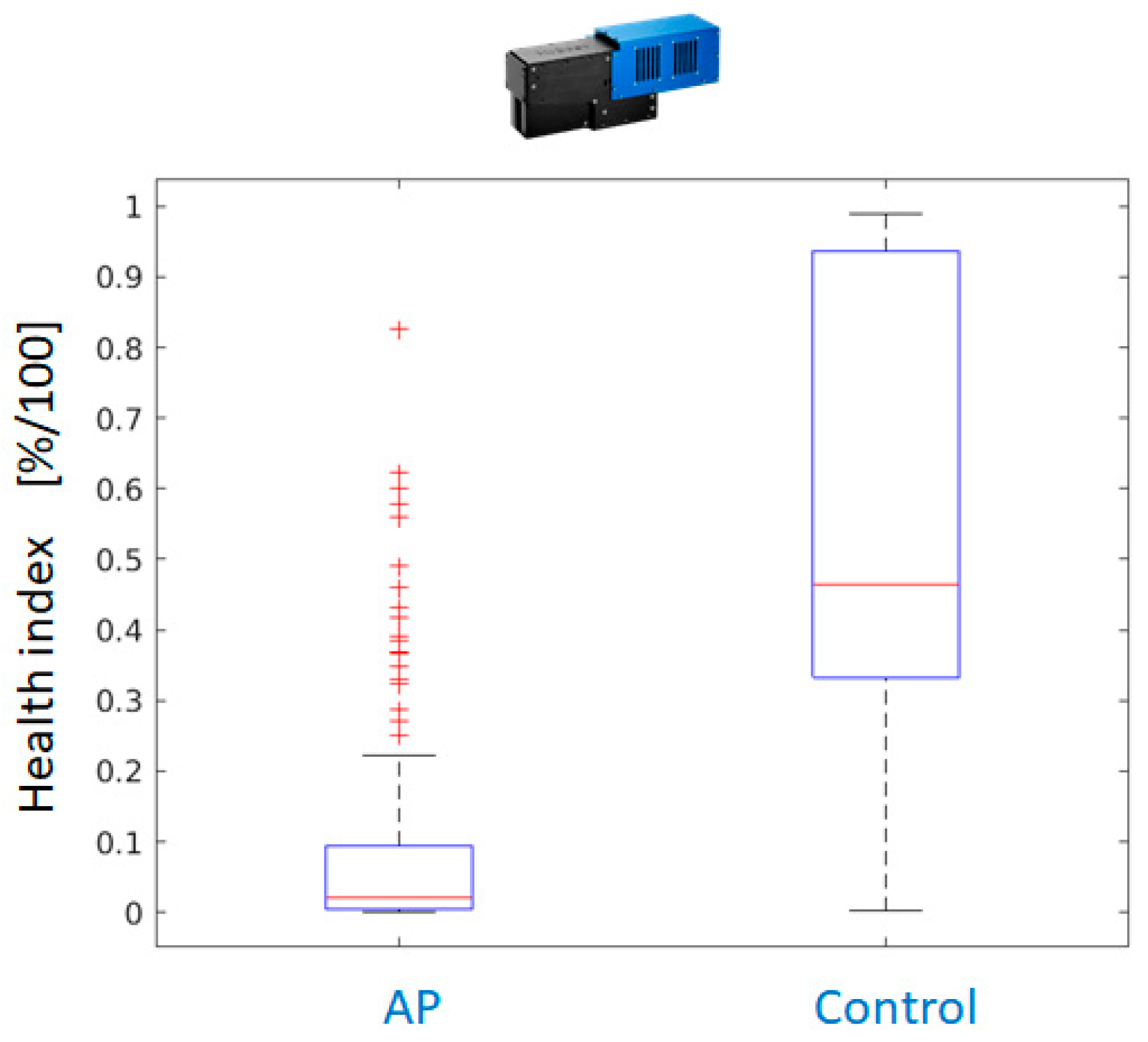
Figure 17 shows the better separation of health index values between AP-infected leaves and healthy control for the VNIR camera. If a threshold of health index 0.25 is applied, only a few leaves of infected trees are falsely classified as healthy and the majority of leaves of healthy trees can be correctly classified.
The field test samples (AP-FTS) in combination with the Random Forest classifier yield additional insights into variable importance.
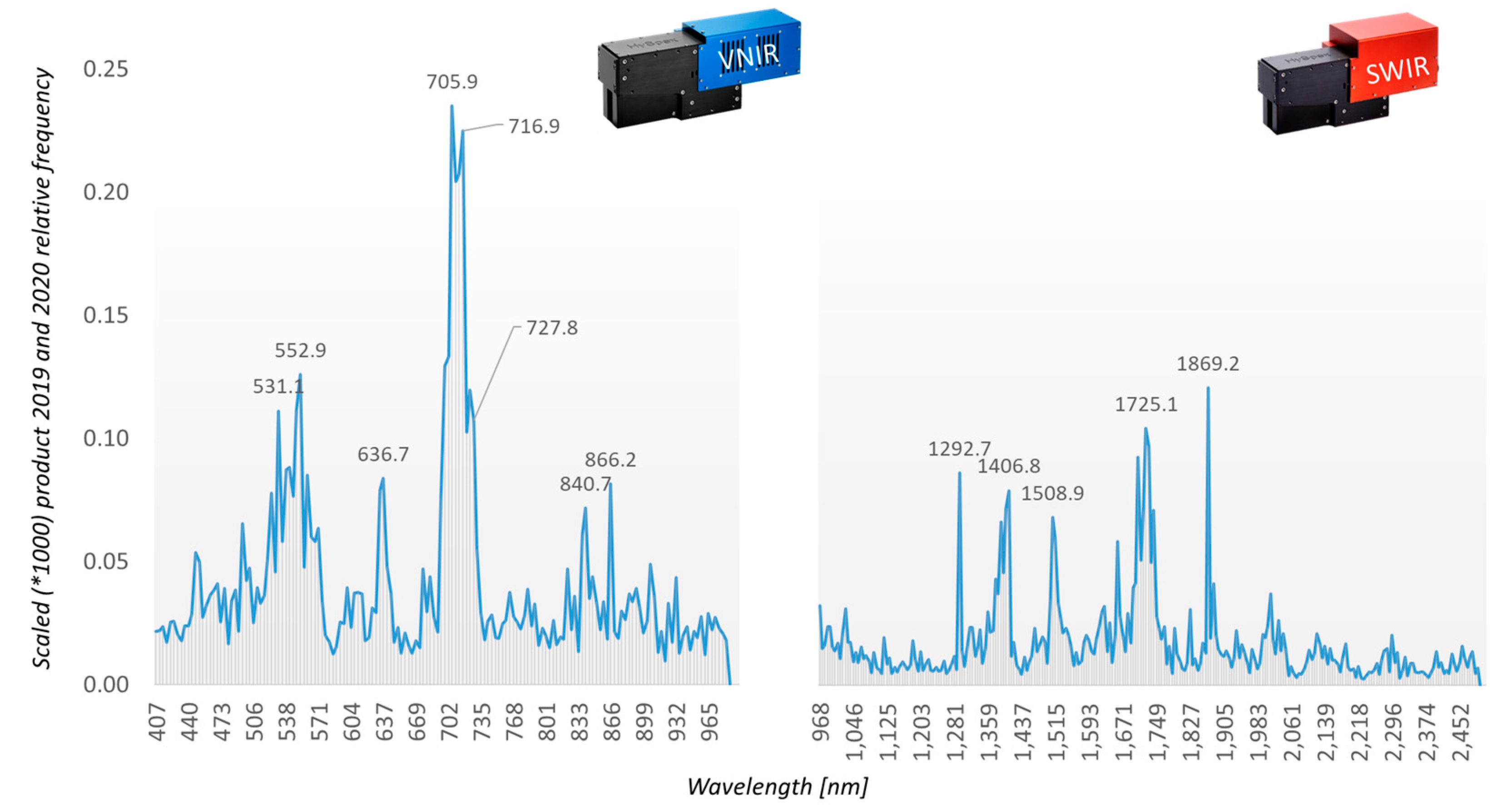
Figure 18 shows the frequency of assessing a certain band in the decisions of the Random Forest.
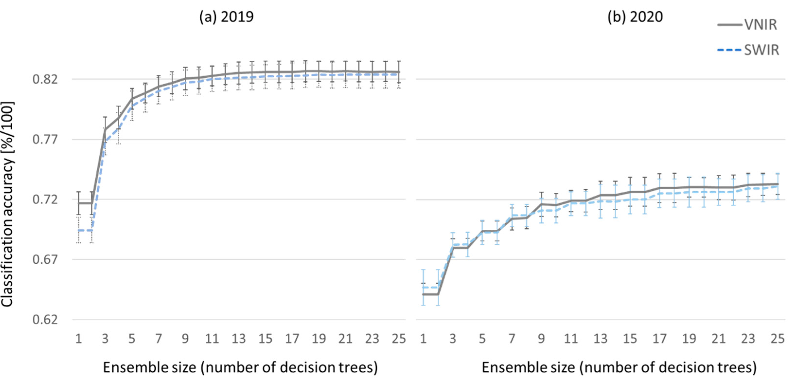
Figure 19 shows the classification accuracies and their standard deviations for different sizes of the Random Forest ensemble classifier. With increasing ensemble size the classification accuracies improves.
To investigate, which camera and which range of the electromagnetic spectrum yields better results, VNIR and SWIR camera data are processed independently.
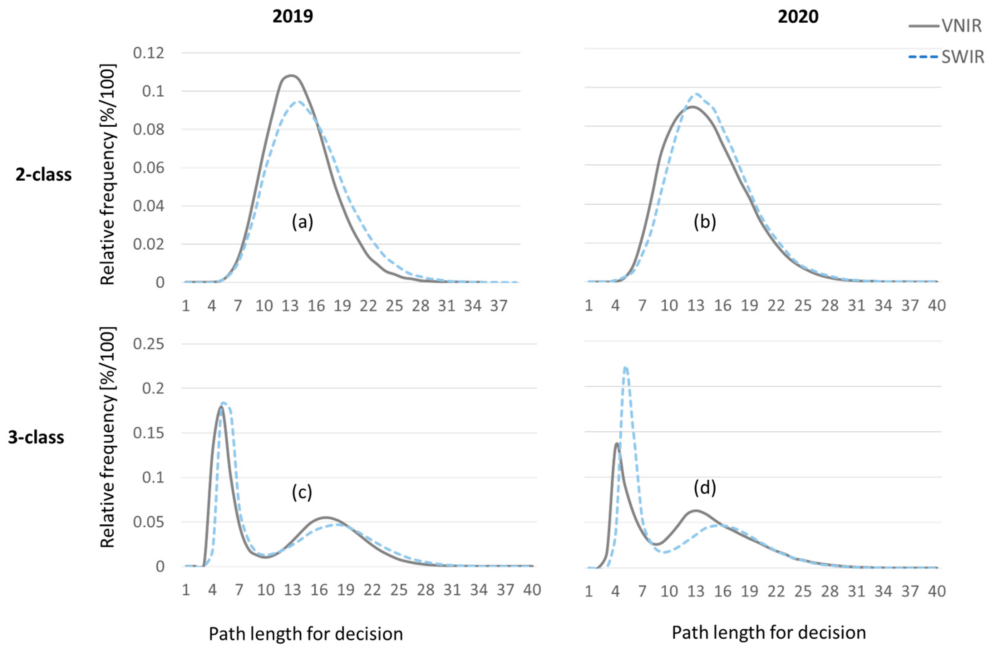
Figure 20 compares the complexity of the pixelwise decisions based on the number of bands per tree that are evaluated for each decision. More difficult decisions correspond to longer path lengths in the decision trees that constitute the Random Forest. Also, longer decision paths from root node to the leave nodes of the decision trees correspond to higher computation times, both in classifier training and classifier recall. The left column of
Figure 20 shows results for the 2019 dataset and the right column for the 2020 dataset, respectively. The upper row shows pathlength distribution for the 2-class problem to discriminate between infected and healthy leaf spectra. As the Random Forest classifier is capable to efficiently tackle multi class problems, the histograms in the lower row represent the 3-class problem to discriminate between the two leaf classes and the image background. Both diagrams for the 3-class problem exhibit a bimodal distribution. The first peak corresponds to detection of the background pixels. Because separation of leaf tissue and metal background is the easier problem, the number of wavelengths to be evaluated is low compared to number of bands used for discrimination between infected and healthy leaf area.
3.5. Spatial-Spectral Classification
A problem-specific dimensionality reduction with LDA and statistical measures for image blocks of different sizes provide an alternate feature space for image segmentation.
Table 8 lists the classification accuracies based on this feature space. Classification of the 2019 dataset is improved by more than 6 percent for both, VNIR and SWIR camera data. For the 2020 dataset, no major improvements are observed. Using spatial-spectral features classification accuracy for both years reaches a similar quality (2019 = 0.751, 2020 = 0.734, see
Table 8) compared to pure spectral classification (2019 = 0.685, 2020 = 0.731, see
Table 7).
4. Discussion
In this article we reported results of ML-based detection of apple proliferation disease. Hyperspectral imaging was used as a means to record data under controlled conditions (illumination, positioning of the leaves). If successful, this setup can be used as an additional lab-based test for diagnosis of the disease. As non-invasive optical measurement, it can potentially outperform PCR tests in terms of sample preparation, required time for testing and sample throughput. Therefore, the study aims to report on detectability of visible (e.g. leaf reddening) and invisible symptoms of apple proliferation. Moreover, results are expected to support implementation of proximal diagnosis in the field by providing information about relevant wavelength bands and an upper bound on expected detection quality given optimal imaging conditions in the laboratory environment.
Analysis of samples from the AP-ITP experiments, where apple trees have been artificially infected and exhibition of symptoms have been studied under different conditions in a climate chamber, showed the highest level of detectability using classification algorithms (AP-ITP, a mean accuracy of 0.971 in 10-fold cross-validation of leaf spectra per pixel with rRBF classifier). However, these experiments were limited to single varieties of apple trees and both, inoculation and measurements took place in a controlled environment. A limited generalization of the results to real-world samples is supported by the findings on spectral indices and separability of infected and healthy tissue. Comparison of AP-ITP-2 and AP-ITP-3 samples exhibit very different distributions of index values for NDVI, CCI, GLI, and PRI between experiments. Within each experiment, a good separation of infected and healthy samples is observed for using mean indices per tree and per leaf instead of indices per pixel. This demonstrates, that leaf symptoms of apple proliferation are not equally spread over the leaf, might be differently distributed on leaves of a single infected tree, and therefore results of pixelwise classification might be always biased towards false detections of the disease, as healthy tissue is present on leaves of infected trees and therefore is potentially included in any training sample. To address this intrinsic problem, several measures have been investigated: using features of leaves and trees instead of pixelwise features, using spatial-spectral features, and using morphological operations on label maps after pixel-wise classification. All mentioned techniques improve results when integrated in the decision process and can be used in combination.
In spectral imaging of vegetation, a coupling between the pattern of reflected light at certain wavelengths and physiological processes and reaction to biotic and abiotic stresses exist. Therefore, the relevance of input features for solving a classification or regression problem allows to analyze underlying processes and differences between classes. For the AP-ITP experiment, the feature relevance after training of a rRBF classifier was extracted. Because 10-fold cross-validation results in 10 different models, the standard deviation of the relevance value was incorporated as an inverse weighting factor. Because neighboring bands of the reflection spectrum of vegetation are highly correlated, random effects like the elements within each fold (training dataset) and random choices in classifier training like initialization parameters lead to slightly different positions of most relevant bands. Therefore, we combined the results of AP-ITP-2 and AP-ITP-3 into a generalized relevance profile (
Figure 9) by multiplying the obtained and weighted relevance profiles of the two datasets. We assume, that this approach better exploits spectral bands of general interest for the AP detection. So far, we did not investigate, which classification performance is achieved, when the input features are limited to a subset of most relevant bands. Interestingly, for the VNIR camera the most relevant bands concentrate in the region of the visible light. Operating a RGB camera with high spatial resolution for AP detection seems feasible. However, the decision process itself uses all available bands and relevance profiles for the individual datasets show importance in the NIR bands, too.
For the AP-FTS experiment, we estimated variable importance by analyzing the decision process within the individual decision trees of the ensemble classifier. The histogram of accessing a certain wavelength band is recorded and used as an importance measure. The relevance profiles of the different years 2019 and 2020 have been combined in a similar way as described for the AP-ITP experiment (
Figure 18). Here, the locations of the obtained most relevant bands are strongly correlated with well-known properties of the reflectance spectra of vegetation, namely the green peak at ~550 nm, a red band at ~637 nm, a number of bands in the red edge region centered at ~706 nm, and NIR bands at ~840 nm and ~866 nm. As the AP-FTS consists of samples from different orchards and apple varieties, these results are promising for application of proximal sensing with multispectral camera systems. The relevance peak at ~637 nm might be correlated to reports of a special red color which a trained human expert can detect on infected trees. It must be noted, that the good classification results depend on more than a single feature, but the design and performance of specialized camera systems for AP detection can benefit from the requirements of the detection algorithms.
We selected only a subset of available classification algorithms to solve the AP detection problem. SVM with different kernels, ensemble classifiers, and the MLP neural network classifier still represent state of the art classifiers for the task of spectral data classification. Single decision trees have been included in our study as control, because the used ensemble classifiers consist of a number of decision trees. So far, deep learning approaches like CNN classifiers have not been investigated for the given problem. Given an extention of the available training dataset, this could be a promising direction of future research. Such research should focus on providing pretrained models for different plant diseases which can then be adapted to novel use cases. However, interpretation of the decision process and relevant features becomes more complicated as model complexity is drastically increased.
In addition to detection of an AP infection based on hyperspectral imaging of the leaves, we investigated regression of qPCR results based on hyperspectral data. While, the achieved RMSE of ~14.5 phytoplasmas per plant cell is promising, spectral data of healthy leaves receive relatively high response values of up to ~25. Therefore, the optical assessment is to sensitive compared to qPCR. If results are combined with a detection threshold and aggregated from leaf to tree level by averaging results of qPCR as well as the optical measurements, a further improvement can be expected. A remaining uncertainty is the question how close the local concentration of phytoplasma and infection symptoms like reddening of a leaf are correlated. We showed in our previous study that the intensity of leaf reddening is not correlated to the phytoplasma titer in the leaf petiole and concluded that the leaf reddening is a long-distance effect of the phytoplasma infection of the tree [
4]. As phytoplasmas are not homogenously distributed in AP-infected trees, molecular detection may be hampered by the small sample size used for diagnosis. In this regard, optical assessment of reddened leaves can be more sensitive than molecular diagnosis [
4].
The phytoplasma infection weakens the tree and induces a multitude of physiological changes. Therefore, specific and unspecific hyperspectral effects are difficult to distinguish and common indices for growth parameters like NDVI achieve already relatively good results. The phytoplasma infection induces a premature chlorophyll breakdown [
7] which leads to a specific leaf reddening due to the presence of the anthocyanin cyanidin-3-glucoside [
32]. This symptom is totally different from leaf senescence in fall and is highly correlated to the presence of the phytoplasma [
4]. Therefore, our results pave the way for a large-scale hyperspectral diagnosis of AP in the field, either in a mobile laboratory or with a portable spectroradiometer as done by Barthel et al. [
9]. Our work is also a prerequisite for the establishment of remote sensing strategies for AP. For this, multi- or hyperspectral data obtained by UAVs or satellites can be used [
33].
5. Conclusions
In this paper, results of a 2-year study of leaf symptoms of AP are reported. They provide the foundation of future research and development towards in-field assessment of AP by optical sensors. We identified most relevant wavelength bands based on machine learning, which can lead to an optimized design of measurement instruments for AP detection. Also, a processing pipeline for hyperspectral images has been proposed and different parameters to improve classification results have been investigated. The use of spatial-spectral features further improves detection quality. Detection quality also benefits from classification of leaves instead of pixels as well as further aggregation of the decisions to decisions per tree.
Author Contributions
Conceptualization, W.J. and U.K.; methodology, U.K., K.H., P.M.; software, U.K, P.M.; validation, U.K., W.J., P.M. and B.T.; formal analysis, U.K., P.M. and B.T.; investigation, W.J. and M.R.; resources, U.K., W.J. and M.R.; data curation, U.K., W.J., K.H. and B.T.; writing—original draft preparation, U.K. and W.J.; writing—review and editing, U.K., W.J., K.H., B.T., P.M., L.K.; visualization, U.K.; supervision, U.K. and W.J.; project administration, U.K., W.J., K.H., B.T., S.W.; funding acquisition, U.K. and W.J. All authors have read and agreed to the published version of the manuscript.
Funding
This research was funded by LANDWIRTSCHAFTLICHE RENTENBANK, grant number 857 727.
Institutional Review Board Statement
Not applicable.
Informed Consent Statement
Not applicable.
Data Availability Statement
Datasets used within this study are available upon request.
Acknowledgments
The authors thank the growers for allowing us access to their orchards for sampling. We are grateful to Anna Kicherer and Nehle Bendel for providing access and help in using the hyperspectral camera system at Julius Kühn-Institute at Siebeldingen. The authors further acknowledge the redesign of the rack-mount for the hyperspectral cameras by David Kilias.
Conflicts of Interest
The authors declare no conflicts of interest. The funders had no role in the design of the study; in the collection, analyses, or interpretation of data; in the writing of the manuscript; or in the decision to publish the results.
References
- Seemüller, E.; Carraro, L.; Jarausch, W.; Schneider, B. Apple Proliferation Phytoplasma. In Virus and Virus-like Diseases of Pome and Stone Fruits; Hadidi, A., Barba, M., Candresse, T., Jelkmann, W., Eds.; APS Press: Saint Paul, MN, USA, 2011; pp. 67–73. ISBN 978-0-89054-396-2. [Google Scholar] [CrossRef]
- Jarausch, B.; Tedeschi, R.; Sauvion, N.; Gross, J.; Jarausch, W. Psyllid vectors. In Phytoplasmas: Plant Pathogenic Bacteria—II. Transmission and Management of Phytoplasma—Associated Diseases; Bertaccini, A., Weintraub, P.G., Rao, G.P., Mori, N., Eds.; Springer: Singapore, 2019; pp. 53–78. [Google Scholar] [CrossRef]
- Barthel, D.; Fischnaller, S.; Letschka, T.; Janik, J.; Mittelberger, C.; Öttl, S.; Panassiti, B.; Angeli, G.; Baldessari, M.; Bianchedi, P.L.; et al. Scopazzi del Melo: Stato Attuale della Ricerca—Apfeltriebsucht: Aktueller Stand der Forschung; Janik, K., Barthel, D., Oppedisano, T., Anfora, G., Eds.; Fondazione Edmund Mach: San Michele all’Adige, Italy; Centro di Sperimentazione Laimburg: Ora, Italy, 2020; pp. 1–153. ISBN 9788878430532. [Google Scholar]
- Jarausch, W.; Runne, M.; Schwind, N.; Jarausch, B.; Knauer, U. Phytoplasma-Induced Leaf Reddening as a Monitoring Symptom of Apple Proliferation Disease with Regard to the Development of Remote Sensing Strategies. Agronomy 2024, 14, 376. [Google Scholar] [CrossRef]
- Mattedi, L.; Forno, F.; Branz, A.; Bragagna, P.; Battocletti, I.; Gualandri, V.; Pedrazzoli, F.; Bianchedi, P.; Deromedi, M.; Filippi, M.; et al. Come riconoscere la malattia in campo: Novità sulla sintomatologia. In Scopazzi del Melo—Apple Proliferation; Ioriatti, C., Jarausch, W., Eds.; Fondazione Edmund Mach: San Michele all’Adige, Italy, 2008; pp. 41–50. [Google Scholar]
- Öttl, S.; Baric, S.; Dalla Via, J. Teilweise Rotfärbung weist nicht auf Apfeltriebsucht hin. Obstbau Weinbau 2008, 2, 58–59. [Google Scholar]
- Mittelberger, C.; Pichler, C.; Yalcinkaya, H.; Erhart, T.; Gasser, J.; Schumacher, S.; Janik, K.; Robatscher, P.; Kräutler, B.; Oberhuber, M. Pathogen-Induced Leaf Chlorosis: Products of Chlorophyll Breakdown Found in Degreened Leaves of Phytoplasma-Infected Apple (Malus × domestica Borkh.) and Apricot (Prunus armeniaca L.) Trees Relate to the Pheophorbide a Oxygenase/Phyllobilin Pathway. J. Agric. Food Chem. 2017, 65, 2651–2660. [Google Scholar] [CrossRef] [PubMed]
- Barthel, D.; Dordevic, N.; Fischnaller, S.; Kerschbamer, C.; Messner, M.; Eisenstecken, D.; Robatscher, P.; Janik, K. Detection of apple proliferation disease in Malus × domestica by near infrared reflectance analysis of leaves. Spectrochim. Acta Part A Mol. Biomol. Spectrosc. 2021, 263, 120178. [Google Scholar] [CrossRef]
- Barthel, D.; Cullinan, C.; Mejia-Aguilar, A.; Chuprikova, E.; McLeod, B.A.; Kerschbamer, C.; Trenti, M.; Monsorno, R.; Prechsl, U.E.; Janik, K. Identification of spectral ranges that contribute to phytoplasma detection in apple trees—A step towards an on-site method. Spectrochim. Acta Part A Mol. Biomol. Spectrosc. 2023, 303, 123246. [Google Scholar] [CrossRef]
- Al-Saddik, H.; Simon, J.C.; Cointault, F. Development of spectral disease indices for ‘Flavescence dorée’ grapevine disease identification. Sensors 2017, 17, 2772. [Google Scholar] [CrossRef]
- Al-Saddik, H.; Simon, J.-C.; Cointault, F. Assessment of the optimal spectral bands for designing a sensor for vineyard disease detection: The case of “Flavescence dorée”. Precis. Agric. 2019, 20, 398–422. [Google Scholar] [CrossRef]
- Bendel, N.; Backhaus, A.; Kicherer, A.; Köckerling, J.; Maixner, M.; Jarausch, B.; Biancu, S.; Klück, H.-C.; Seiffert, U.; Voegele, R.T.; et al. Detection of Two Different Grapevine Yellows in Vitis vinifera Using Hyperspectral Imaging. Remote Sens. 2020, 12, 4151. [Google Scholar] [CrossRef]
- Jarausch, B.; Schwind, N.; Fuchs, A.; Jarausch, W. Characteristics of the spread of apple proliferation by its vector Cacopsylla picta. Phytopathology 2011, 101, 1471–1480. [Google Scholar] [CrossRef]
- Lenhard, K.; Baumgartner, A.; Schwarzmaier, T. Independent Laboratory Characterization of NEO HySpex Imaging Spectrometers VNIR-1600 and SWIR-320m-e. IEEE Trans. Geosci. Remote Sens. 2015, 53, 4–1828. [Google Scholar] [CrossRef]
- Knauer, U.; von Rekowski, C.S.; Stecklina, M.; Krokotsch, T.; Pham Minh, T.; Hauffe, V.; Kilias, D.; Ehrhardt, I.; Sagischewski, H.; Chmara, S.; Seiffert, U. Tree Species Classification Based on Hybrid Ensembles of a Convolutional Neural Network (CNN) and Random Forest Classifiers. Remote Sens. 2019, 11, 2788. [Google Scholar] [CrossRef]
- Knauer, U.; Matros, A.; Petrovic, T.; Zanker, T.; Scott, E.S.; Seiffert, U. Improved classification accuracy of powdery mildew infection levels of wine grapes by spatial-spectral analysis of hyperspectral images. Plant Methods 2017, 13, 47. [Google Scholar] [CrossRef]
- Jolliffe, I.T. Principal Component Analysis. Springer Series in Statistics, 2002. [CrossRef]
- MacQueen, J.B. Some methods for classification and analysis of multivariate observations. Proceedings of the 5th Berkeley symposium on mathematical statistics and probability, 1967, 1, pp. 281–297.
- Breiman, L. Random Forests. Mach. Learn. 2001, 45, 5–32. [Google Scholar] [CrossRef]
- Grieco, M.; Schmidt, M.; Warnemünde, S.; Backhaus, A.; Klück, H.-C.; Garibay, A.; Moya, Y.A.T.; Jozefowicz, A.M.; Mock, H.-P.; Seiffert, U.; Maurer, A.; Pillen, K. Dynamics and genetic regulation of leaf nutrient concentration in barley based on hyperspectral imaging and machine learning. Plant Sci. 2022, 315, 111123. [Google Scholar] [CrossRef] [PubMed]
- Bendel, N.; Kicherer, A.; Backhaus, A.; et al. Evaluating the suitability of hyper- and multispectral imaging to detect foliar symptoms of the grapevine trunk disease Esca in vineyards. Plant Methods 2020, 16, 142. [Google Scholar] [CrossRef] [PubMed]
- Fritzke, B. A growing neural gas network learns topologies. In Proceedings of the 7th International Conference on Neural Information Processing Systems (NIPS’94), Denver CO, USA, 1 January 1994; pp. 625–632. [Google Scholar]
- Huang, S.; Tang, L.; Hupy, J.P.; et al. A commentary review on the use of normalized difference vegetation index (NDVI) in the era of popular remote sensing. J. For. Res. 2021, 32, 1–6. [Google Scholar] [CrossRef]
- Davidson, C.; Jaganathan, V.; Sivakumar, A.N.; Czarnecki, J.M.P.; Chowdhary, G. NDVI/NDRE prediction from standard RGB aerial imagery using deep learning. Comput. Electron. Agric. 2022, 203, 107396. [Google Scholar] [CrossRef]
- Kohzuma, K.; Hikosaka, K. Physiological validation of photochemical reflectance index (PRI) as a photosynthetic parameter using Arabidopsis thaliana mutants. Biochem. Biophys. Res. Commun. 2018, 498, 1–52. [Google Scholar] [CrossRef]
- El-Shikha, D.E.; Barnes, E.; Clarke, T.; Hunsaker, D.; Haberland, J.; Pinter, P.; Waller, P.; Thompson, T.L. Remote Sensing of Cotton Nitrogen Status Using the Canopy Chlorophyll Content Index (CCCI). Trans. ASABE 2008, 51, 73–82. [Google Scholar] [CrossRef]
- Gobron, N.; Pinty, B.; Verstraete, M.M.; Widlowski, J.-L. Advanced vegetation indices optimized for up-coming sensors: Design, performance, and applications. IEEE Trans. Geosci. Remote Sens. 2000, 38(6), 2489–2505. [Google Scholar] [CrossRef]
- Lorenz, K.H.; Schneider, B.; Ahrens, U.; Seemüller, E. Detection of the apple proliferation and pear decline phytoplasmas by PCR amplification of ribosomal and nonribosomal DNA. Phytopathology 1995, 85, 771–776. [Google Scholar] [CrossRef]
- Jarausch, W.; Peccerella, T.; Schwind, N.; Jarausch, B.; Krczal, G. Establishment of a quantitative real-time PCR assay for the quantification of apple proliferation phytoplasmas in plants and insects. Acta Hort. 2004, 657, 415–420. [Google Scholar] [CrossRef]
- Liebenberg, A. Influence of latent apple viruses on Malus sieboldii-derived apple proliferation resistant rootstocks. Thesis, Heidelberg University, Heidelberg, Germany, 2013; p. 165. [Google Scholar] [CrossRef]
- Kononenko, I.; Šimec, E.; Robnik-Šikonja, M. Overcoming the Myopia of Inductive Learning Algorithms with RELIEFF. Appl. Intell. 1997, 7, 39–55. [Google Scholar] [CrossRef]
- Zorer, R.; Bianchedi, P.L.; Mattedi, L.; Branz, A. Arrossamento fogliare autunnale. Relazioni con la presenza del fitoplasma e possibili utilizzi nel monitoraggio prossimale o remoto. In Scopazzi del Melo—Apple Proliferation; Ioriatti, C., Jarausch, W., Eds.; Fondazione Edmund Mach: San Michele all’Adige, Italy, 2008; pp. 51–62. [Google Scholar]
- Jarausch, W.; Menz, P.; Al Masri, A.; Runne, R.; Thielert, B.; Kohler, K.; Warnemünde, S.; Kilias, D.; Jarausch, B.; Knauer, U. Digital Phytoplasmology: Remote sensing of fruit tree phytoplasma diseases. Phytopath. Mollicutes 2023, 13, 135–136. [Google Scholar] [CrossRef]
Figure 1.
Overview of the data collection and spectral imaging approach. In the AP-FTS experiment each tree is represented by 4 leaves (a), leaves are scanned with hyperspectral cameras (b), and undergo PCR analysis (c), which is then used as reference data for machine learning and data analysis (d).
Figure 2.
Dual camera setup at RLP AgroScience. Measurement system with cameras, light sources, moving stage in a rack-mounted setup (a) and in operation (b).
Figure 2.
Dual camera setup at RLP AgroScience. Measurement system with cameras, light sources, moving stage in a rack-mounted setup (a) and in operation (b).
Figure 3.
Visualizations of the hyperspectral image data. (a) Single channel intensity image of SWIR 320m-e data with false color information layer (detected leaf area), (b) hyperspectral image cube with color-coded radiance data.
Figure 3.
Visualizations of the hyperspectral image data. (a) Single channel intensity image of SWIR 320m-e data with false color information layer (detected leaf area), (b) hyperspectral image cube with color-coded radiance data.
Figure 4.
Prediction of qPCR values based on regression. The mean spectrum of individual leaves from the VNIR camera served as predictors, while the corresponding qPCR results for the leaves served as the target variable.
Figure 4.
Prediction of qPCR values based on regression. The mean spectrum of individual leaves from the VNIR camera served as predictors, while the corresponding qPCR results for the leaves served as the target variable.
Figure 5.
Mean spectra of healthy and infected leaves with per band standard deviation of reflectance plotted for experiment AP-ITP-2.
Figure 5.
Mean spectra of healthy and infected leaves with per band standard deviation of reflectance plotted for experiment AP-ITP-2.
Figure 6.
Mean spectra of healthy and infected leaves with per band standard deviation of reflectance plotted for experiment AP-ITP-3.
Figure 6.
Mean spectra of healthy and infected leaves with per band standard deviation of reflectance plotted for experiment AP-ITP-3.
Figure 7.
Variance weighted relevance of individual bands for the rRBF classifier and the AP-ITP-2 dataset.
Figure 7.
Variance weighted relevance of individual bands for the rRBF classifier and the AP-ITP-2 dataset.
Figure 8.
Variance weighted relevance of individual bands for the rRBF classifier and the AP-ITP-3 dataset.
Figure 8.
Variance weighted relevance of individual bands for the rRBF classifier and the AP-ITP-3 dataset.
Figure 9.
Combined relevance of individual bands for the rRBF classifier and all datasets.
Figure 9.
Combined relevance of individual bands for the rRBF classifier and all datasets.
Figure 10.
Scatterplots of selected spectral indices per pixel.
Figure 10.
Scatterplots of selected spectral indices per pixel.
Figure 11.
Scatterplots of aggregated spectral indices (a) minimum value per leaf, (b) average value per tree and (c) minimum value per tree (AP-ITP-2).
Figure 11.
Scatterplots of aggregated spectral indices (a) minimum value per leaf, (b) average value per tree and (c) minimum value per tree (AP-ITP-2).
Figure 12.
Scatterplots of selected spectral indices per pixel for experiment AP-ITP-3.
Figure 12.
Scatterplots of selected spectral indices per pixel for experiment AP-ITP-3.
Figure 13.
Scatterplots of aggregated spectral indices (a) minimum value per leaf, (b) average value per tree and (c) minimum value per tree (AP-ITP-3).
Figure 13.
Scatterplots of aggregated spectral indices (a) minimum value per leaf, (b) average value per tree and (c) minimum value per tree (AP-ITP-3).
Figure 14.
Comparison of confusion matrices for 2020 SWIR dataset AP-FTS. The stars denote the best obtained TPR for the two classes. Operating points correspond to equal misclassification cost. Models correspond to best performing models from
Table 7 (last column) for each method category.
Figure 14.
Comparison of confusion matrices for 2020 SWIR dataset AP-FTS. The stars denote the best obtained TPR for the two classes. Operating points correspond to equal misclassification cost. Models correspond to best performing models from
Table 7 (last column) for each method category.
Figure 15.
ROC curves for best performing ML algorithms on the 2020 SWIR dataset AP-FTS. (a) ROC curve for detection of healthy leaf tissue, (b) ROC curve for detection of leaf tissue of infected trees. Operating points correspond to equal misclassification cost. Models correspond to best performing models from
Table 7 (last column) for each method category. Random Forest classifier outperforms other models in the ROC space as indicated by maximum AUC measure.
Figure 16.
Boxplots with a comparison of disease detection quality for (a) VNIR, (b) SWIR, (c) combined decision based on the fraction of affected surface used as a health index.
Figure 16.
Boxplots with a comparison of disease detection quality for (a) VNIR, (b) SWIR, (c) combined decision based on the fraction of affected surface used as a health index.
Figure 17.
Separation between healthy and AP infected trees is improved by digital image processing (DILATION with a 5x5 rectangular kernel to emphasize healthy regions).
Figure 17.
Separation between healthy and AP infected trees is improved by digital image processing (DILATION with a 5x5 rectangular kernel to emphasize healthy regions).
Figure 18.
Relevance measure of individual bands (frequency of use in decisions for the whole dataset) obtained for AP-FTS.
Figure 18.
Relevance measure of individual bands (frequency of use in decisions for the whole dataset) obtained for AP-FTS.
Figure 19.
Pixelwise classification accuracies (infected vs. healthy leaf tissue) for different numbers of decision trees in Random Forest classifiers show better classification performance for AP-FTS data from VNIR hyperspectral camera and all ensemble sizes in years (a) 2019 and (b) 2020.
Figure 19.
Pixelwise classification accuracies (infected vs. healthy leaf tissue) for different numbers of decision trees in Random Forest classifiers show better classification performance for AP-FTS data from VNIR hyperspectral camera and all ensemble sizes in years (a) 2019 and (b) 2020.
Figure 20.
Complexity of decision indicated by path lengths (wavelength bands evaluated during a single decision) of unpruned decision trees. Using VNIR data, decisions are found with less comparisons in both years, 2019 and 2020, compared to SWIR data. Detection of background as 3rd class requires less operations than classification of leaf tissue.
Table 1.
Origin, cultivar and health status of apple leaf samples analyzed in AP-FTS.
Table 1.
Origin, cultivar and health status of apple leaf samples analyzed in AP-FTS.
| Region |
|
2019 |
|
2020 |
|
| Orchard code |
Cultivar |
N°
symptomatic leaves |
N°
healthy leaves |
N°
symptomatic leaves |
N°
healthy leaves |
| Vorderpfalz |
|
|
|
|
|
| Nied1 |
Golden Delicious |
12 |
4 |
32 |
8 |
| NW5 |
Rubinette |
40 |
4 |
8 |
16 |
| NW13 |
Ambasie |
8 |
4 |
|
|
| NW13 |
Axam |
16 |
0 |
|
|
| NW14 |
Delbarestivale |
24 |
0 |
16 |
36 |
| NW14 |
Falstaff |
20 |
0 |
|
|
| NW14 |
Jonagold |
16 |
0 |
4 |
4 |
| NW14 |
Pink Lady |
20 |
0 |
|
|
| NW14 |
Pinova |
20 |
4 |
16 |
16 |
| NW14 |
Rubinola |
20 |
4 |
4 |
24 |
| NW14 |
Topaz |
52 |
4 |
44 |
8 |
| NW16 |
unknown |
72 |
24 |
|
|
| NW17 |
Berlepsch |
24 |
0 |
|
|
| NW17 |
Boskoop |
36 |
4 |
|
|
| NW17 |
Fuji Yataka |
12 |
0 |
|
|
| NW17 |
Gala |
16 |
0 |
28 |
12 |
| NW17 |
Idared |
0 |
4 |
|
|
| NW17 |
Jonagold |
32 |
0 |
24 |
4 |
| NW17 |
Melrose |
24 |
0 |
|
|
| NW17 |
Pinova |
8 |
0 |
|
|
| Südpfalz |
|
|
|
|
|
| 47e |
Golden Delicious |
|
|
52 |
0 |
| KKA1 |
Gala |
40 |
0 |
4 |
0 |
| KKA1 |
Jonagold |
28 |
0 |
|
|
| IlbA1 |
unknown |
20 |
8 |
|
|
| IlbA3 |
unknown |
|
|
4 |
0 |
| IlbA7 |
unknown |
|
|
8 |
0 |
| LeiA4 |
Delbarestivale |
4 |
0 |
|
|
| LeiA4 |
Gala |
16 |
0 |
|
|
| LeiA4 |
Pilot |
0 |
4 |
|
|
| LeiA4 |
Pinova |
4 |
0 |
|
|
| LeiA7 |
Braeburn |
12 |
0 |
8 |
4 |
| LeiA7 |
Celest |
16 |
4 |
|
|
| LeiA7 |
Gala Royal |
24 |
0 |
28 |
0 |
| LeiA7 |
Pilot |
20 |
0 |
4 |
0 |
| LeiA7 |
Rubinette |
16 |
0 |
|
|
| total |
|
672 |
72 |
284 |
132 |
Table 2.
Overview and comparison of the parameters of the used hyperspectral imaging sensors. VNIR 1800 and SWIR 384 are used in a dual camera setup for AP-ITP-1, VNIR 1600 and SWIR 320m-e are used for AP-ITP-2, AP-ITP-3 and AP-FTS.
Table 2.
Overview and comparison of the parameters of the used hyperspectral imaging sensors. VNIR 1800 and SWIR 384 are used in a dual camera setup for AP-ITP-1, VNIR 1600 and SWIR 320m-e are used for AP-ITP-2, AP-ITP-3 and AP-FTS.
| |
VNIR 1800 |
VNIR 1600 |
SWIR 384 |
SWIR 320m-e |
| Spectral range [nm] |
400–1000 |
416–992 |
930–2500 |
968–2497 |
| Spatial pixels |
1800 |
1600 |
384 |
320 |
| Spectral bands |
186 |
160 |
288 |
256 |
| Spectral sampling [nm] |
3.26 |
3.6 |
5.45 |
6 |
| Framerate [fps] |
260 |
135 |
400 |
100 |
| Radiometric quantization [bit] |
16 |
12 |
16 |
14 |
Table 3.
Selected spectral indices for assessment of tree health. The abbreviation R800 denotes reflectance value in band with central wavelength of 800 nm.
Table 3.
Selected spectral indices for assessment of tree health. The abbreviation R800 denotes reflectance value in band with central wavelength of 800 nm.
| Spectral index |
Definition |
Reference |
| Normalized difference vegetation index (NDVI) |
(R800 − R670)/(R800 + R670) |
Huang et al. (2020) [23] |
| Normalized difference red edge (NDRE) 1
|
(R790 – R720)/(R790+R720) |
Davidson et al. (2022) [24] |
| Physiological reflectance index (PRI) |
(R531 − R570)/(R531 + R570) |
Kohzuma et al. (2018) [25] |
| (Canopy) chlorophyll content index (CCI) |
NDRE/NDVI |
El-Shikha et al. (2008) [26] |
| Green leaf index (GLI) |
(2*R550-R650-R440)/ (2*R550+R650+R440) |
Gobron et al. (2000) [27] |
Table 4.
Comparison of selected regression algorithms for prediction of qPCR values from spectral imaging data (experiment AP-ITP-1).
Table 4.
Comparison of selected regression algorithms for prediction of qPCR values from spectral imaging data (experiment AP-ITP-1).
| Method |
Hyperparameters |
Preselection |
PCA |
Features |
RMSE |
| Linear regression |
|
RReliefF (20) |
x |
10 |
17.76 |
| |
none |
x |
10 |
16.867 |
| Ensemble of regression trees |
Bagging (Random Forest) |
RReliefF (20) |
x |
10 |
17.596 |
| |
none |
x |
5 |
19.793 |
| Support Vector Regression |
Linear kernel |
RReliefF (20) |
x |
10 |
18.143 |
| |
none |
x |
10 |
16.867 |
| Gaussian kernel (scale 3.2) |
RReliefF (20) |
x |
10 |
16.345 |
| |
MRMR (20) |
x |
10 |
16.698 |
| Gaussian Process Regression |
Exponential GPR |
RReliefF (20) |
x |
10 |
14.491 |
| |
none
none
none
F-test (20)
MRMR (20)
RReliefF (20) |
x
x
x
x |
186
5
10
10
10
20 |
17.968
17.438
15.938
18.5
16.195
18.138 |
Table 5.
Confusion matrix (10-fold cross-validation) of best performing classification method (rRBF with relative Euclidian distance) for pixelwise classification (accuracy 0.971) for the VNIR data.
Table 5.
Confusion matrix (10-fold cross-validation) of best performing classification method (rRBF with relative Euclidian distance) for pixelwise classification (accuracy 0.971) for the VNIR data.
| |
Infected |
Healthy |
| Infected |
0.983 |
0.017 |
| Healthy |
0.041 |
0.959 |
Table 6.
Confusion matrix (10-fold cross-validation) of best performing classification method (rRBF with relative Euclidian distance) for pixelwise classification (accuracy 0.971) for the SWIR data.
Table 6.
Confusion matrix (10-fold cross-validation) of best performing classification method (rRBF with relative Euclidian distance) for pixelwise classification (accuracy 0.971) for the SWIR data.
| |
Infected |
Healthy |
| Infected |
0.972 |
0.028 |
| Healthy |
0.029 |
0.971 |
Table 7.
Overview of the classification performance for the 2-class problem (healthy vs. AP infected) in stratified dataset AP-FTS (10-fold cross-validation, mean accuracy).
Table 7.
Overview of the classification performance for the 2-class problem (healthy vs. AP infected) in stratified dataset AP-FTS (10-fold cross-validation, mean accuracy).
| Method |
Hyperparameters |
VNIR 2019 |
VNIR 2020 |
SWIR 2019 |
SWIR 2020 |
| Decision Tree |
GINI diversity index, max 100 splits |
0.639 |
0.66 |
0.624 |
0.688 |
| GINI diversity index, max 20 splits |
0.645 |
0.656 |
0.617 |
0.676 |
| GINI diversity index, max 4 splits |
0.603 |
0.641 |
0.597 |
0.665 |
| Ensembles of decision trees |
Bagging (Random Forest) |
0.673 |
0.7 |
0.645 |
0.731 |
| Boosting |
0.665 |
0.676 |
0.642 |
0.697 |
| Support Vector Machines |
linear kernel |
0.654 |
0.662 |
0.634 |
0.71 |
| quadratic kernel |
0.664 |
0.7 |
0.685 |
0.728 |
| cubic kernel |
0.653 |
0.676 |
0.646 |
0.713 |
| Gaussian kernel |
0.678 |
0.7 |
0.65 |
0.708 |
Neural Networks
10 neurons per layer, ReLU, Bayesian optimization |
1 layer |
0.631 |
0.678 |
0.662 |
0.721 |
MLP 2 layers
MLP 3 layers |
0.652
0.644 |
0.676
0.682 |
0.66
0.659 |
0.728
0.723 |
Table 8.
Overview of the classification results for the 2-class problem (healthy vs. AP infected) in stratified dataset AP-FTS.
Table 8.
Overview of the classification results for the 2-class problem (healthy vs. AP infected) in stratified dataset AP-FTS.
| Method |
Hyperparameters |
VNIR 2019 |
VNIR 2020 |
SWIR 2019 |
SWIR 2020 |
| Decision Tree |
GINI diversity index, max 100 splits |
0.7 |
0.69 |
0.693 |
0.709 |
| GINI diversity index, max 20 splits |
0.689 |
0.689 |
0.676 |
0.723 |
| GINI diversity index, max 4 splits |
0.672 |
0.687 |
0.662 |
0.714 |
| Ensembles of decision trees |
Bagging (Random Forest) |
0.741 |
0.693 |
0.751 |
0.731 |
| Boosting |
0.696 |
0.694 |
0.686 |
0.734 |
| Support Vector Machines |
linear kernel |
0.654 |
0.689 |
0.67 |
0.733 |
| quadratic kernel |
0.673 |
0.686 |
0.702 |
0.729 |
| cubic kernel |
0.599 |
0.537 |
0.7 |
0.715 |
| Gaussian kernel |
0.738 |
0.702 |
0.751 |
0.733 |
Neural Networks
10 neurons per layer, ReLU, Bayesian optimization |
1 layer |
0.704 |
0.695 |
0.697 |
0.713 |
MLP 2 layers
MLP 3 layers |
0.714
0.718 |
0.698
0.698 |
0.702
0.7 |
0.71
0.711 |
| Improvement over spectral analysis |
|
+0.063 |
+0.002 |
+0.066 |
+0.003 |
|
Disclaimer/Publisher’s Note: The statements, opinions and data contained in all publications are solely those of the individual author(s) and contributor(s) and not of MDPI and/or the editor(s). MDPI and/or the editor(s) disclaim responsibility for any injury to people or property resulting from any ideas, methods, instructions or products referred to in the content. |
© 2024 by the authors. Licensee MDPI, Basel, Switzerland. This article is an open access article distributed under the terms and conditions of the Creative Commons Attribution (CC BY) license (https://creativecommons.org/licenses/by/4.0/).
