1. Introduction
Real-time monitoring of building operations has been a key factor in optimizing the energy systems in a building to normalize building operation. Traditional energy optimization strategies involved real-time anomaly correction, manual scheduling, and experts’ judgement based on the specific infrastructure and properties of the building [
1]. Data-driven techniques based on machine learning have started gaining the attention of building managers because of these techniques’ strength in analyzing complex historical consumption patterns, hence providing analytical insights to support preventive decision making. Building energy demand data obtained through a variety of time-sensitive sensors can be used to anticipate future patterns such as peak demand periods. Hence, demand prediction models are becoming increasingly essential for reducing costs, mitigating risks, and improving overall operational efficiency [
2]. It turns out that prediction models need to be carefully designed such that the resulting system will be able to take into consideration different historical scenarios in the energy consumption profile and provide insights into the future with sufficient accuracy and reliability. It is also helpful for building managers to have a model that quantifies uncertainty, enabling them to verify the reliability of the predictions to make more accurate decisions. Based on the type of insights a model provides, there are basically two approaches in demand prediction models, namely, deterministic approaches and probabilistic approaches.
Models trained with a deterministic approach provide a precise estimate of the response variable by assuming that it has a fixed relationship with predictor variables that generally represents a central tendency in the data. Therefore, the goal of a deterministic training approach is to estimate relationship parameters (or weights) while minimizing the loss function, which calculates the average distance between the observed values and the predicted values. The training process is computationally efficient, and precise predictions can be generated without any additional analysis of the model weights. There exist various machine learning-based deterministic prediction models for predicting demand that excel in precision, computational efficiency, and simplicity.
Since electricity and HVAC demands are highly non-linear in nature, a deterministic model is expected to capture the non-linearity, hence improving the prediction accuracy for both short- and long-term predictions. Deterministic models such as those based on traditional machine learning (ML) and deep learning (DL) show significant prediction accuracy for both short-term and long-term demand predictions [
3,
4,
5] focused on the traditional ML-based models such as boosting, random forests, and support vector machines for short-term HVAC and electricity demand prediction. The results highlight that these types of models are good at generalization on unseen data with less training effort. Additionally, [
5] proves the superiority of tree-based algorithms over artificial neural networks in prediction accuracy. However, conventional ML generally lacks the ability to model complex input-output relationships, which is a key advantage in various DL models. Several studies have revealed that DL models are better at modeling response variables compared with conventional ML, with little preprocessing effort and domain knowledge required. For example, [
6,
7,
8] proposed LSTM, CNN, and gated recurrent unit (GRU)-based models that are accurate in modeling long-term temporal dependencies, which are limited through traditional ML. Several studies [
9,
10] showed concern over the limited learning capabilities in simple DL models, hence introducing hybrid DL architectures. In a hybrid setting, the advantages of multiple ML- and DL-based models are combined in hopes of improving generalization on unseen data with compromises to training time and resources. However, models based on a deterministic approach lack representation of the inherent uncertainty and its impact on the response variable, which is crucial in many applications, especially in demand prediction. Additionally, hybrid deterministic models are far more complex than single models, and therefore it is difficult to trace the model’s prediction path. Deterministic DL models are often referred to as “black box” models, which means that there is no or limited opportunity to interpret the internal weight representation. Deep neural networks excel in prediction accuracy, but because of the longer training time it is nearly impossible to experimentally confirm the model’s performance over the whole parameter space.
Many successful prediction models that quantify uncertainty are based on Bayesian learning and are referred to as the probabilistic approach to prediction models. Unlike the deterministic approach, probabilistic prediction models do not imply a fixed relationship of predictors with the response variable. Additionally, the probabilistic approach offers flexibility to a model during training by approximating variances and deviations in the data, which makes the model capture complex relationships. That is why recent studies have introduced techniques to incorporate uncertainty in various deterministic demand prediction models [
11,
12,
13]. Studies such as [
14,
15,
16,
17,
18,
19] deep dive into the analysis of uncertainty quantification in Bayesian-based DL models, and stochastic models are highly precise in predictions and appropriate for decision making. For example, Bayesian-based LSTM [
14] and stochastic models [
17] have shown capabilities to predict for the long-term, which is beneficial in provisioning the energy management. Bayesian-based models are also capable of calibrating the parameters of physics-based energy models [
15] and are accurate and highly beneficial for simulating large energy models. Bayesian-based models can also be viewed as a special case of Gaussian process (GP) models, which are greatly beneficial in modeling complex relationships between gas and electricity consumption when trained on relatively smaller time series data [
16]. Results of another study [
18] also indicated that when Bayesian-based models are adopted in hierarchical fashion, they result in a robust representation of data across different spatial levels with accurate uncertainty quantification. Finally, Bayesian-based neural networks [
19] can learn complex relationships between variables across different scales of data collection frequencies (Ex. 15-minutes, hourly) and spatial levels (Ex. individual or all households in a region). Overall, all studies conclude that Bayesian-based models are capable of modeling complex relationships with a variety of stochastic variables, with specific attention to uncertainty quantification, which fosters communication between the users and the prediction models. Additionally, they also help to avoid overreliance on the model predictions and to make risk-aware decisions. Moreover, probabilistic models can represent uncertainty in weight distribution as well as in prediction; therefore, they offer high trustworthiness for various demand prediction tasks.
Electricity and HVAC demand prediction is a challenging task since various external factors introduce uncertainty, which is difficult to quantify through a deterministic approach. Therefore, we have proposed in this study a Bayesian neural network (BNN)-based probabilistic model for building-level electricity and heating, ventilation, and cooling (HVAC) demand prediction. Various BNN models are trained on real-world building operations data and are compared against long short-term memory (LSTM) models with Monte Carlo (MC) dropout, or MC-LSTM. Unlike normal dropouts with fixed probability, MC dropout randomly generates a dropout mask during training that introduces stochasticity into the model [
20,
21]. The MC dropout also helps avoid overfitting and increases the generalization ability of the LSTM. Our results showed that the BNN-based models outperformed the MC-LSTM models, with significant performance improvement in quantifying uncertainty and prediction accuracy. The major contributions of this study are listed as follows.
A BNN-based model is proposed for hourly prediction of energy demand in a real-world building.
The impact of various hyperparameters that can affect the uncertainty estimation during training are analyzed and presented in a detailed discussion based on various evaluation metrics.
Fixed-horizon validation is performed using various prediction horizons like 1-day, 1-week, and 1-month to assess the reliability of short- and long-term predictions. The generalization is also assessed by testing models on a full-length test dataset.
A comprehensive comparison is performed between BNN and MC-LSTM over the uncertainty quantification and prediction accuracy.
The rest of the content of this paper is organized in the following manner:
Section 2 outlines the system model by introducing the building parameters, the models under investigation, and the benchmarks.
Section 3 outlines the dataset, the experiment settings, and a detailed empirical comparative analysis on the overall training and validation results. We conclude our study in section 4. Code can be found at:
https://github.com/punarvas/IESL/tree/main/power_forecast (last accessed: September 09, 2024).
3. Numerical Results
3.1. Dataset of the Building Energy Demand
In this study, a subset of the 3-year building operations performance dataset for Building 59 [
22] was used to train and evaluate various models for predicting electricity and HVAC demand. In addition to selected time series features from the dataset, several temporal features were derived that contribute during the training process. The selected time series originally had multiple missing data points. We already know that the data are aggregated on an hourly frequency for this study. This section outlines the general information on the dataset along with detailed preprocessing steps.
Each time series in the final dataset ranges from 2018-01-01 (1:00) to 2020-12-31 (7:00) and has exactly 26,287 hours of data. The following detailed preprocessing steps were carried out to obtain the final dataset:
First, an index of timestamps from 2018-01-01 to 2020-12-31 is created and each time series is joined to its corresponding timestamp. This process reveals missing timestamp entries.
For each time series, the missing values are filled by copying the value from the previous hours to preserve the long-term variability in the data, which might get hindered if missing values are imputed with series mean or median.
Features such as season and weekend status are derived from the timestamp since usage in the electricity and HVAC are varied throughout weekends and seasons in California.
Event in progress is derived from the timeline of the maintenance and environmental events reported in the dataset description [
3]. Duty status is derived from the building’s work hours found on LBNL’s official website.
Autocorrelation analysis is performed for the electricity and HVAC time series to quantify the dependency of the current timestamp on that of the previous timestamp. Analysis reveals a strong correlation of each time series with its 24-hour and 168-hour lagged value.
Binary variables and categorical variables are transformed to one-hot encoded vectors, which eases the learning process.
Original statistical properties such as mean and standard deviation are stored separately for later use for the response variables of electricity and HVAC. Log-transformation and Z-normalization are performed on the electricity and HVAC time series.
Table 1 shows the variables in our final dataset used for training and validation.
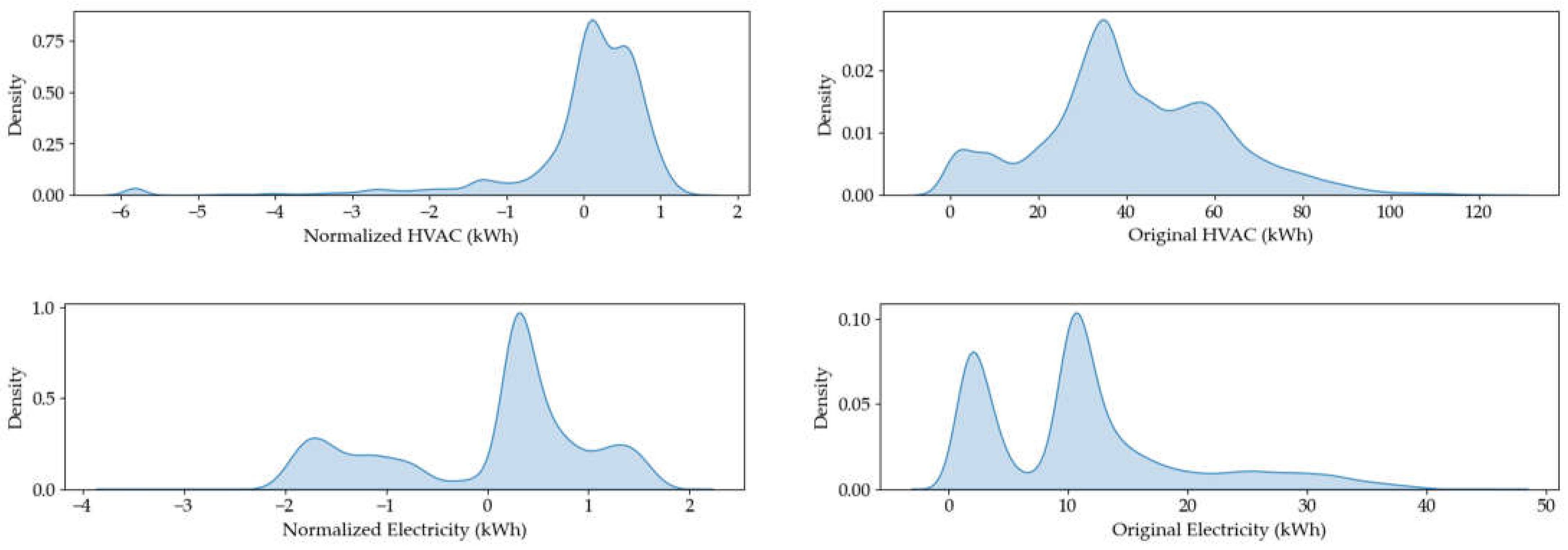
Figure 3 shows the data distribution of response variables before and after the preprocessing.
For complex models such as BNN and MC-LSTM, providing a maximum number of examples will avoid overfitting as well as improve the generalization ability. Since maximum possible examples are provided during training, these models will be able to precisely represent the variability and inherent noise in the dataset. Hence, all models were trained on the approximately 2 years and 6 months of training dataset and evaluated on 6 months of test dataset. Additionally, a larger training dataset could also provide more insights into the unique characteristics of the Building 59 dataset, allowing for more accurate conclusions. This study also evaluates the performance of BNN and MC-LSTM for their short- and long-term predictions through a fixed-horizon validation technique, in which models are evaluated on multiple varying-length test datasets, namely, 1-day, 1-week, and 1-month. For understanding the effect of training configuration on model performance, hyperparameter tuning in terms of batch size and learning rate was performed and evaluation results were reported for each size of test dataset. All models were trained on two thousand epochs and optimized using an Adam optimizer with an exponential learning rate scheduler to adapt the learning rate dynamically throughout the long-term learning process, which further avoided local minima. Negative log-likelihood loss (NLL) was used as a loss function during training of BNN-based models.
3.2. Training and Evaluation
This section outlines the results of the systematic training and evaluation process for QRF, MC-LSTM, and BNN. A detailed comparative analysis on the results is outlined in section 3.3.
3.2.1. QRF-Based Models
Table 2 shows the summary of evaluations of QRF-based electricity and HVAC models.
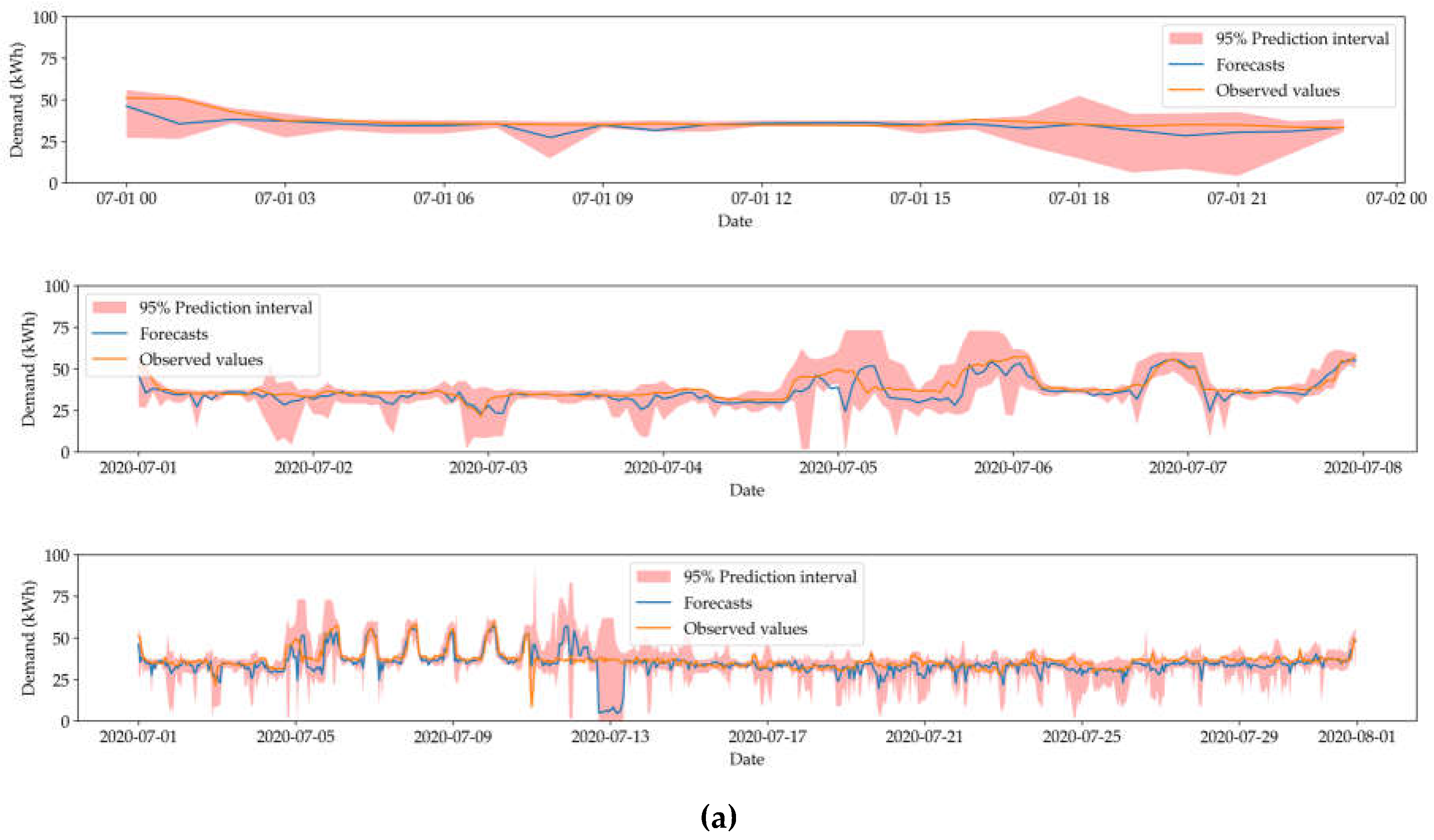
Figure 4 shows the corresponding visualizations for the best results.
3.2.2. LSTM-Based Models
Table 3 and
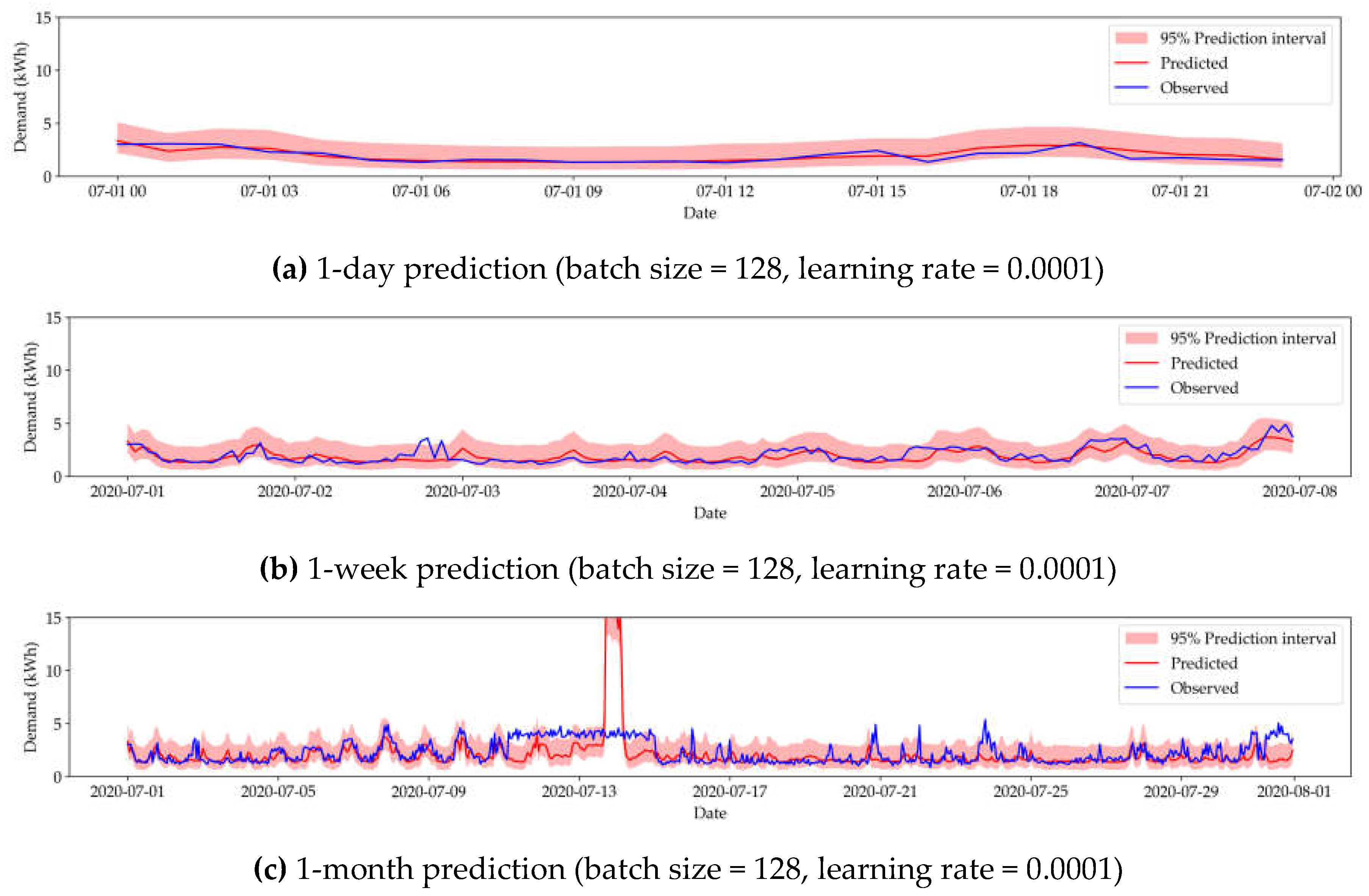
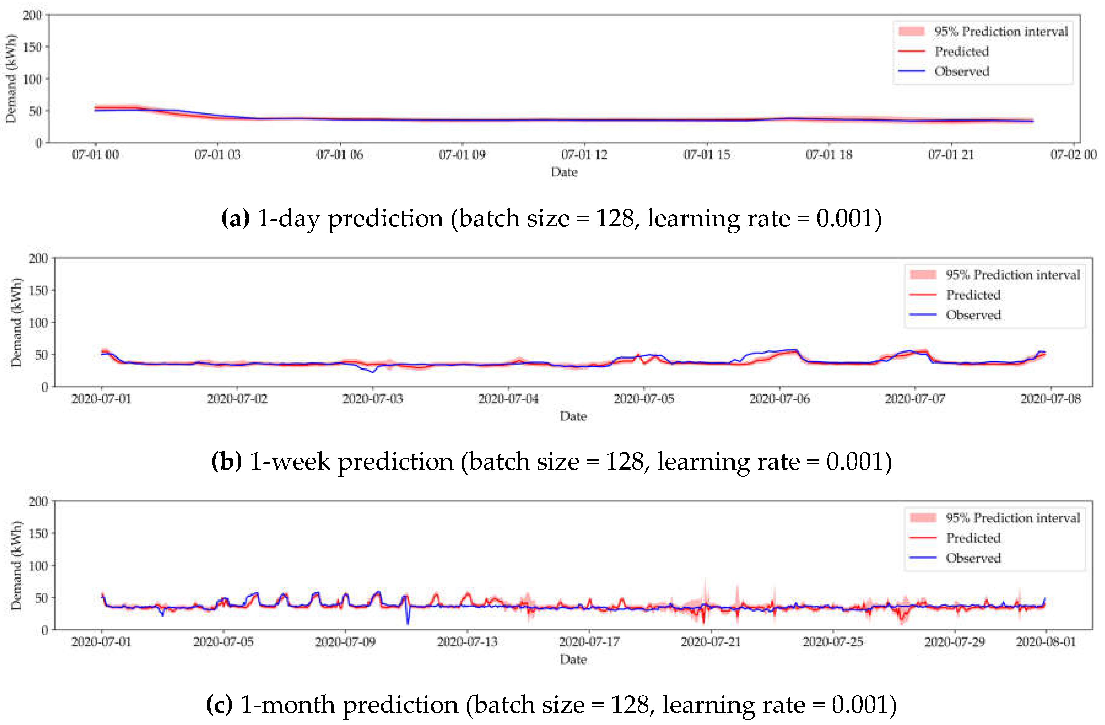
Table 4 show the summary of evaluation of the MC-LSTM-based HVAC and electricity models, respectively. Corresponding time series visualizations for the best results can be found in
Appendix A.1.
3.2.3. BNN-Based Models
Table 5 and
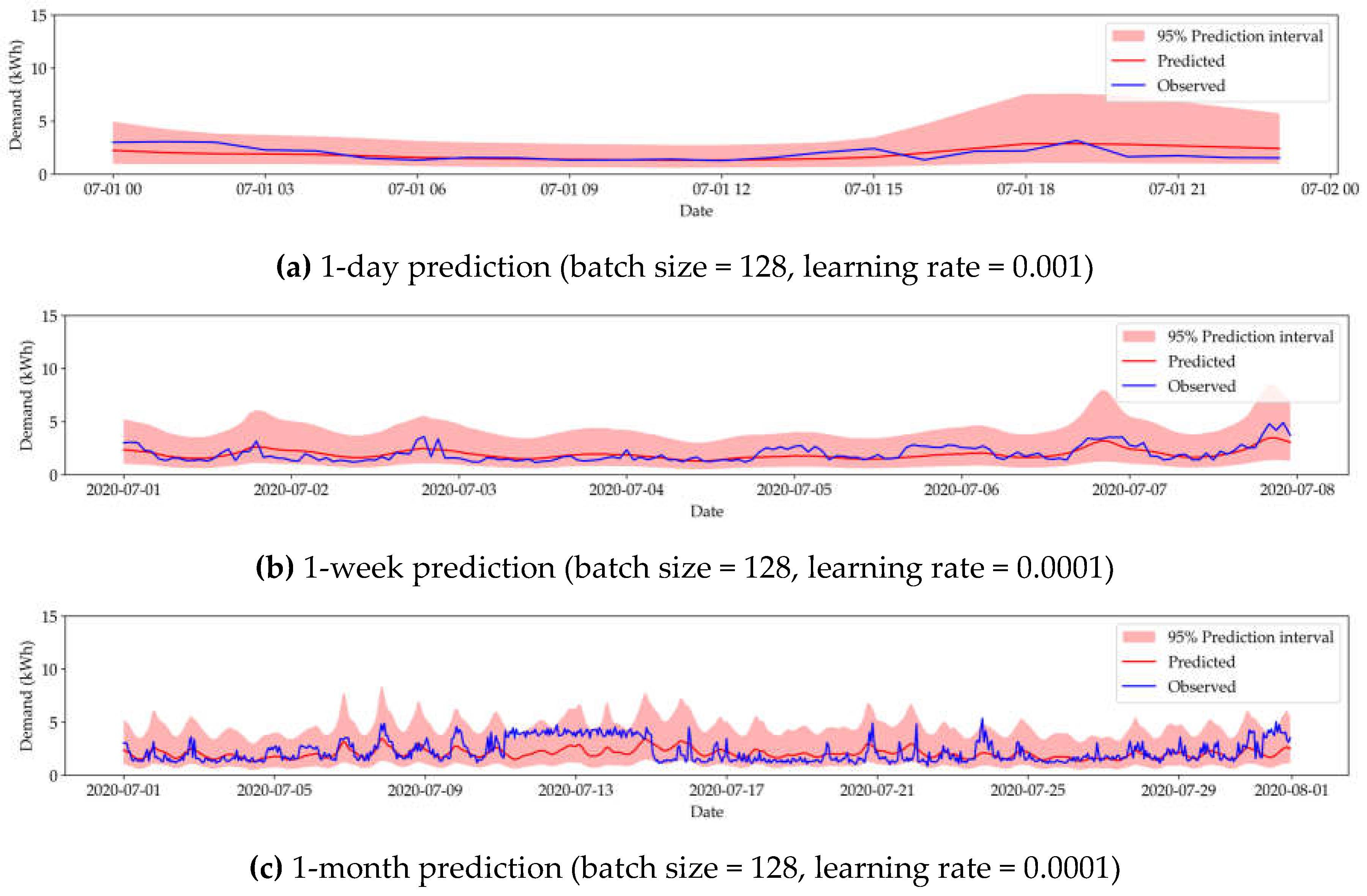
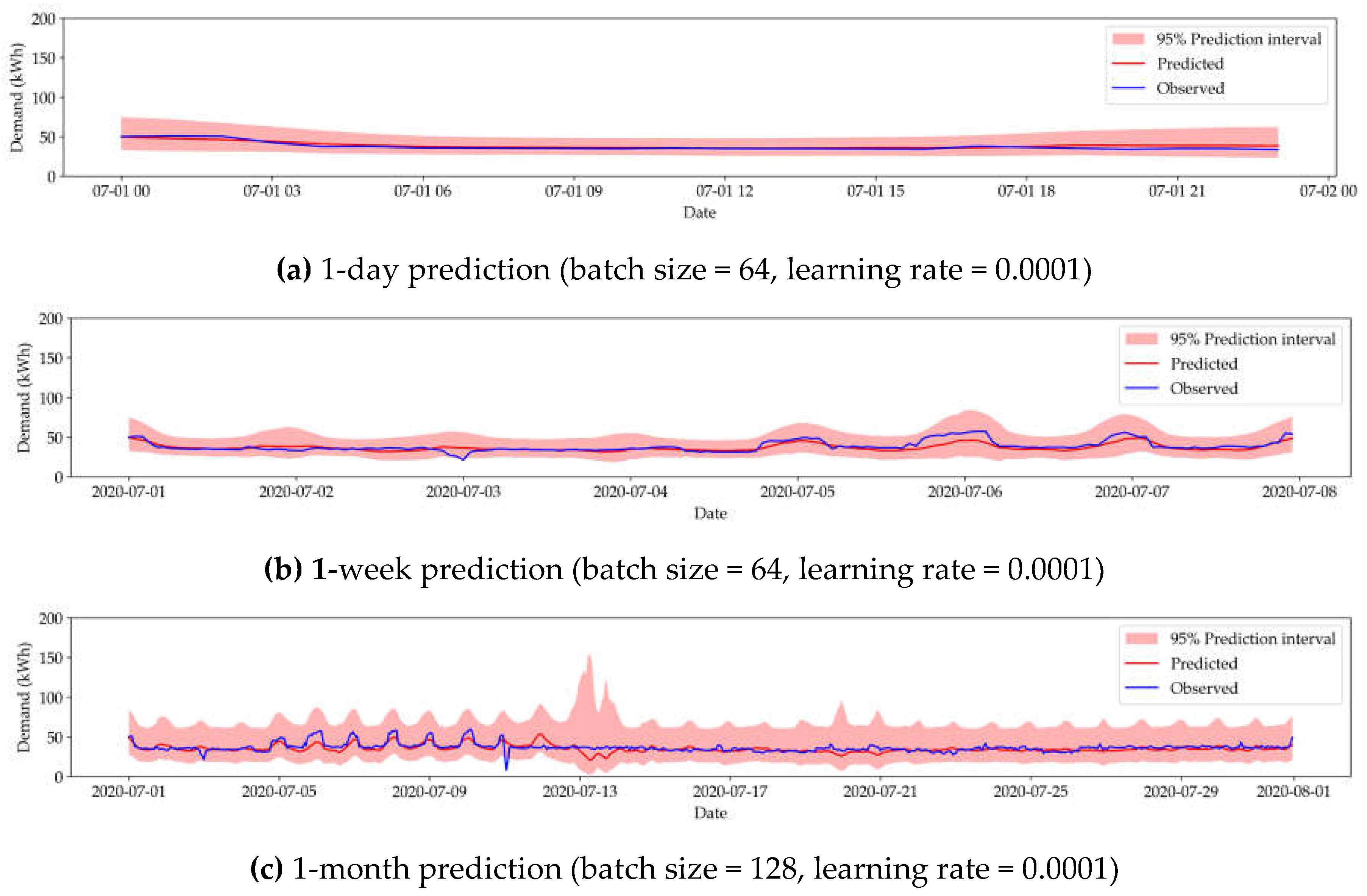
Table 6 show the summary of tests on BNN-based HAC and electricity models, respectively. Corresponding visualizations for the best results can be found in
Appendix A.2.
3.3. Comparative Analysis
In this section, a thorough comparison of the performance metrics of the MC-LSTM-based and BNN-based HVAC and electricity models is performed. The comparison prioritizes the uncertainty quantification in both the variants over the deterministic prediction evaluation metrics.
Table 7 and
Table 8 show comparisons of the HVAC and electricity models alongside the benchmark results. For ease of comparison, we have highlighted the best metrics in bold.
In nearly all the cases, MC-LSTM-based models have outperformed BNN-based models in terms of prediction accuracy. This is because of the inherent property of the underlying LSTM to adapt the long-term dependencies, especially in the time series dataset. On the other hand, BNN-based models have performed excellently in uncertainty quantification, characterized by metrics like PICP, CRPS, MPIW, and NLL. In certain cases of short-term electricity predictions (1-day and 1-week), MC-LSTM showed the best uncertainty quantification, which indicates that LSTM is suitable for short-term predictions. BNN-based HVAC models had the best metrics, which was a key comparison factor since the HVAC time series is relatively noisier than the electricity time series. Therefore, it is evident that BNN-based models are potentially robust to noisy data.
Clearly, additional evidence was required to select the best-suited variant for both of the response variables since deterministic evaluation metrics on short-term test datasets like 1-day and 1-week did not provide sufficient information on the model’s generalization capabilities. Long-term predictions (1-month and more) provided a general view of the performance metrics because of the data volume and variety of examples involved. Performance of the BNN and MC-LSTM variants was compared across different prediction horizons using MAPE, which offered an insight into relative growth in the prediction error as the size of the dataset grew. From
Table 7 and
Table 8, it can be observed that MC-LSTM-based models have gradually introduced more errors into their predictions as the length of the prediction horizon increased. To intensify the significance of these errors, the performance of MC-LSTM and BNN-based models was outlined for the complete test dataset in
Table 9, which provided a more precise and general measure of the errors and uncertainty estimation.
From
Table 9, it is evident that for a complete test dataset, BNN-based models have outperformed MC-LSTM-based models in uncertainty quantification and prediction accuracy. MC-LSTM also significantly deviated in estimating the posterior distribution of the dataset characterized by the NLL and MPIW. It turns out that MC-LSTM-based models were overconfident during long-term predictions characterized by the PICP. On the other hand, BNN-based models accounted for the variations in the full test dataset that did not accurately reflect in the 1-day, 1-week, and 1-month evaluations. One potential explanation for why the BNN-based models outperformed MC-LSTM in prediction accuracy can be drawn from the model’s complexity, training parameters, and architecture. As already mentioned, BNN- and MC-LSTM-based models share a common layered architecture during training. Our findings also revealed that BNN-based models did not show a significant sensitivity toward the different hyperparameters, which was not true about the MC-LSTM-based models, which showed a significant change in performance as the training parameters changed. However, it is important to explore various combinations of hyperparameters while training BNN-based models for a different application.
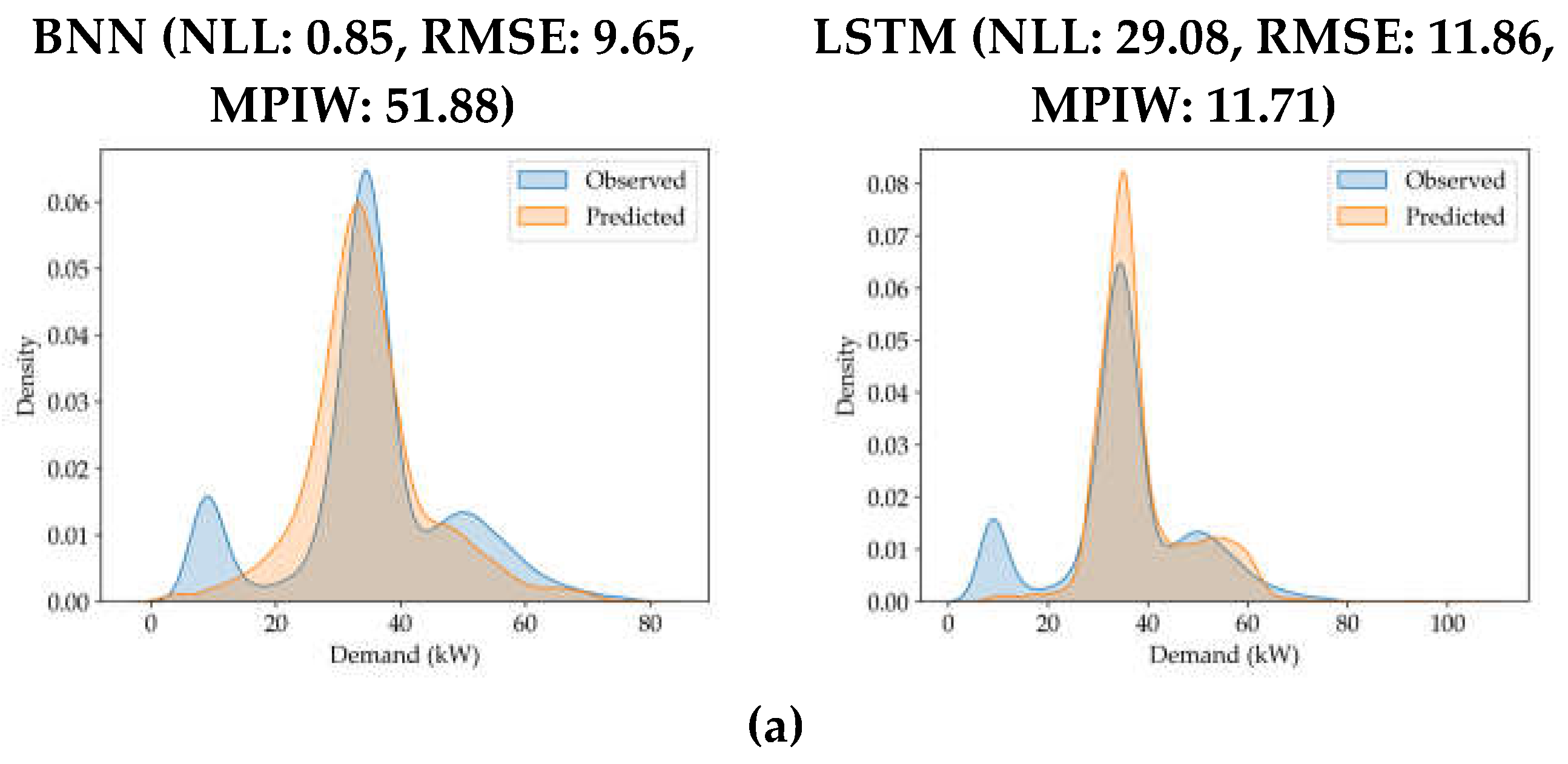
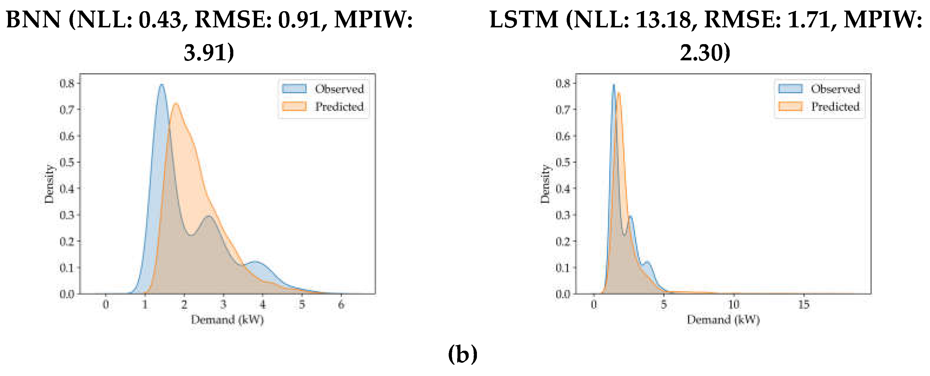
It is necessary to visually inspect the resulting predictions alongside the evaluation metrics to make informed decisions in real-world situations. Unlike BNN-based models, prediction of MC-LSTM-based models has narrow prediction intervals, especially for long-term predictions. Although the MC-LSTM-based model achieved satisfactory performance in prediction accuracy, it is also necessary to have MPIW and NLL to be proportionate. Higher MPIW with low NLL suggest a good estimation of the uncertainty but a sacrifice of the accuracy characterized by the deterministic evaluation metrics. This factor was evident in the results for both BNN and MC-LSTM. This argument was supported by visualizing the kernel density estimation (KDE) plots for the actual values and the predicted values for both BNN- and MC-LSTM-based models. If the breadth of the KDE of the actual values and predicted values are closer to each other, the model has accounted for the uncertainty in the test dataset. If the KDE of actual values is higher than the KDE of the predicted values, then there is a sign of overconfidence and vice versa. The KDE plots are visualized for the selected models for the complete test dataset in
Figure 5.
KDE plots provided additional insights into the uncertainty estimation in the BNN and MC-LSTM. In
Figure 5(a), BNN-based models have better estimated the distribution of the test dataset compared with the results of the MC-LSTM-based models. MC-LSTM-based models have clearly underestimated the uncertainty in the test dataset. In
Figure 5(b), the breadth of the KDE plot for MC-LSTM-based models was extremely higher than the breadth of the actual values. By visually inspecting the KDE plots of predictions and actual values, it also turns out that a low NLL value did not necessarily guarantee a good fit.
Finally, we would like to highlight a special observation about the BNN-based HVAC models, namely, the tall spikes in the prediction interval during complete test dataset prediction, outlined in
Figure 6.
The spikes do not appear early during the prediction and gradually start intensifying as the length of the series grows. The spiked prediction interval essentially indicates the higher uncertainty in the prediction, which could be the result of sudden data drift in electricity demand during the lockdown period of COVID-19, since electricity demand was incorporated as a predictor variable during the training of the HVAC models. Although this study does not delve into the specifics of data drift, it acknowledges its impact on uncertainty quantification. Further investigation into data drift could provide additional insights into handling such anomalies more effectively.
4. Conclusion
Predicting the building-level energy demand is a beneficial contribution to building management and resourcing. Accurate prediction of the energy demand can provide insights into the demand patterns and hence can potentially help building managers to devise energy consumption policies and make relevant informed decisions. In this study, BNN-based and MC-LSTM-based HVAC and electricity demand prediction models are compared in terms of uncertainty quantification and prediction accuracy. A subset of the building performance dataset for Building 59, which is located inside Lawrence Berkeley National Laboratory, was selected along with some temporal features and building characteristic features. A systematic hyperparameter tuning was performed to explore the performance of the models under various training circumstances and tests performed over various prediction horizons.
Results showed that BNN-based models excel in uncertainty quantification as well as prediction accuracy, outperforming MC-LSTM-based models. The study also revealed that that while MC-LSTM-based models are a good fit for short-term predictions, they lack the uncertainty quantification that is a crucial aspect of predicting the demand for electricity and HVAC. It was also observed that BNN-based models have provided reasonable attention to the prediction confidence characterized by the MPIW. Finally, we addressed a special case on the behavior of BNN-based HVAC models. By reasonably compromising certain deterministic evaluation metrics, BNN-based models can be potential solutions for building-level energy demand prediction. With sufficient computing resources and additional exploration based on the dataset and hyperparameter space, researchers can use the findings from our study to establish robust probabilistic prediction models based on BNN.
Author Contributions
Conceptualization, V.-H.B. and A.M.; methodology, A.M. and V.-H.B.; software, A.M.; validation, W.S. and S.D.; formal analysis, A.M.; investigation, S.D. and W.S.; resources, A.M.; data curation, A.M. and S.D.; writing—original draft preparation, A.M.; writing—review and editing, V.-H.B., S.D., and W.S.; visualization, A.M.; supervision, V.-H.B. and W.S.; project administration, V.-H.B.; funding acquisition, V.-H.B.; All authors have read and agreed to the published version of the manuscript.
Figure 1.
Total electricity and HVAC demand.
Figure 1.
Total electricity and HVAC demand.
Figure 2.
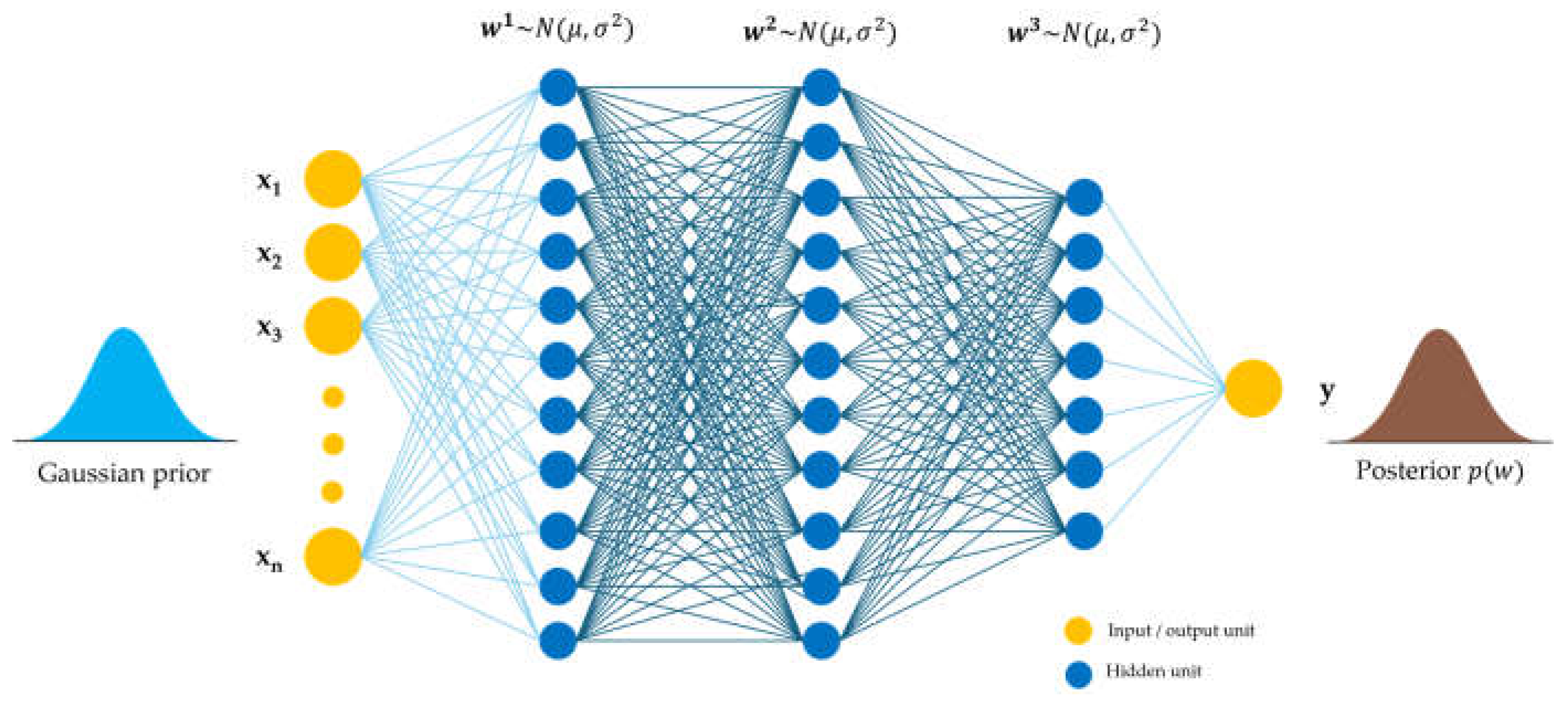
Schematic diagram of a BNN.
Figure 2.
Schematic diagram of a BNN.
Figure 3.
Data distribution HVAC (top) and electricity (bottom) time series before and after preprocessing (right to left).
Figure 3.
Data distribution HVAC (top) and electricity (bottom) time series before and after preprocessing (right to left).
Figure 4.
Time series visualization of (a) day, week, and month HVAC prediction (top to bottom), (b) day, week, and month electricity prediction (top to bottom).
Figure 4.
Time series visualization of (a) day, week, and month HVAC prediction (top to bottom), (b) day, week, and month electricity prediction (top to bottom).
Figure 5.
Kernel Density Estimation plot for actual values and predicted values of (a) HVAC (b) electricity on complete test dataset.
Figure 5.
Kernel Density Estimation plot for actual values and predicted values of (a) HVAC (b) electricity on complete test dataset.
Figure 6.
Observed tall spikes during prediction of HVAC demand on complete test dataset.
Figure 6.
Observed tall spikes during prediction of HVAC demand on complete test dataset.
Table 1.
Variables in the final dataset
Table 1.
Variables in the final dataset
| Variable name |
Type |
Brief description |
| Timestamp |
Date & time |
Reference index for datapoints. This value is not used during training and evaluation of any model. |
| Season |
Categorical |
Season of the year (spring, summer, autumn, winter) |
| Weekend status |
Binary |
True if current timestamp belongs to a weekend (Saturday and Sunday) else False |
| Duty status |
Binary |
True if the current timestamp belongs to the working hours of NBNL (8:00 to 17:00) else False |
| Event in progress |
Binary |
True if there is an ongoing building maintenance or extreme weather/environment event |
| Interior zone temperature |
Continuous |
Average interior temperature of each office zone on the ground and second floor |
| Solar radiation |
Continuous |
Active solar radiation nearby the office building |
| Relative humidity |
Continuous |
Relative humidity nearby the office building |
| Air temperature |
Continuous |
Observed air temperature |
| Wind speed |
Continuous |
Observed wind speed |
| Electricity |
Continuous |
Averaged electricity load across ground and first floor of the office building |
| HVAC |
Continuous |
Averaged HVAC load across ground and first floor of the office building |
Table 2.
Performance summary of quantile regression forest.
Table 2.
Performance summary of quantile regression forest.
| Model |
Period |
Test metrics |
| PICP↑ |
MPIW↓ |
MAE↓ |
RMSE↓ |
MAPE↓ |
| HVAC |
1-day |
0.57 |
1.24 |
0.61 |
0.82 |
0.17 |
| 1-week |
0.48 |
1.18 |
0.77 |
1.03 |
0.14 |
| 1-month |
0.49 |
1.43 |
0.90 |
1.20 |
0.23 |
| Electricity |
1-day |
0.82 |
14.74 |
4.20 |
6.43 |
0.07 |
| 1-week |
0.60 |
17.08 |
7.77 |
10.49 |
0.08 |
| 1-month |
0.70 |
16.37 |
6.14 |
9.30 |
0.10 |
Table 3.
Performance summary of MC-LSTM for predicting HVAC demand.
Table 3.
Performance summary of MC-LSTM for predicting HVAC demand.
| Prediction horizon |
Batch size |
Learning rate |
Test metrics |
| PICP↑ |
CRPS↓ |
MPIW↓ |
NLL↓ |
MAE↓ |
RMSE↓ |
MAPE↓ |
| Day |
64 |
0.001 |
0.58 |
0.07 |
5.03 |
17.35 |
3.45 |
4.80 |
0.09 |
| 0.0001 |
0.79 |
0.03 |
4.48 |
-1.29 |
1.33 |
1.87 |
0.04 |
| 128 |
0.001 |
0.88 |
0.03 |
8.19 |
-1.55 |
1.31 |
2.11 |
0.03 |
| 0.0001 |
0.75 |
0.03 |
4.36 |
-1.16 |
1.71 |
2.05 |
0.04 |
| Week |
64 |
0.001 |
0.53 |
0.11 |
5.68 |
9.09 |
4.86 |
7.18 |
0.12 |
| 0.0001 |
0.72 |
0.04 |
4.98 |
0.26 |
2.03 |
2.95 |
0.05 |
| 128 |
0.001 |
0.83 |
0.05 |
8.41 |
-0.34 |
2.70 |
3.98 |
0.07 |
| 0.0001 |
0.59 |
0.05 |
5.17 |
1.63 |
2.56 |
3.35 |
0.07 |
| Month |
64 |
0.001 |
0.53 |
0.12 |
6.42 |
10.73 |
4.69 |
7.61 |
0.13 |
| 0.0001 |
0.64 |
0.07 |
5.31 |
5.39 |
3.06 |
5.15 |
0.09 |
| 128 |
0.001 |
0.81 |
0.08 |
10.69 |
0.96 |
3.57 |
5.31 |
0.10 |
| 0.0001 |
0.59 |
0.07 |
5.29 |
3.35 |
3.17 |
5.15 |
0.09 |
Table 4.
Performance summary of MC-LSTM for predicting electricity demand.
Table 4.
Performance summary of MC-LSTM for predicting electricity demand.
| Prediction horizon |
Batch size |
Learning rate |
Test metrics |
| PICP↑ |
CRPS↓ |
MPIW↓ |
NLL↓ |
MAE↓ |
RMSE↓ |
MAPE↓ |
| Day |
64 |
0.001 |
0.29 |
0.86 |
3.39 |
84.64 |
4.37 |
7.33 |
2.51 |
| 0.0001 |
0.92 |
0.16 |
2.34 |
0.35 |
0.44 |
0.60 |
0.24 |
| 128 |
0.001 |
0.79 |
0.18 |
2.19 |
0.44 |
0.51 |
0.65 |
0.28 |
| 0.0001 |
1.00 |
0.12 |
2.50 |
-0.04 |
0.30 |
0.38 |
0.15 |
| Week |
64 |
0.001 |
0.54 |
0.54 |
3.23 |
31.51 |
2.64 |
5.43 |
1.27 |
| 0.0001 |
0.91 |
0.17 |
2.29 |
0.23 |
0.45 |
0.63 |
0.22 |
| 128 |
0.001 |
0.88 |
0.18 |
2.08 |
0.54 |
0.51 |
0.72 |
0.25 |
| 0.0001 |
0.98 |
0.14 |
2.48 |
0.10 |
0.38 |
0.52 |
0.19 |
| Month |
64 |
0.001 |
0.50 |
0.50 |
3.01 |
29.95 |
2.23 |
4.34 |
1.05 |
| 0.0001 |
0.82 |
0.23 |
2.39 |
0.67 |
0.68 |
0.98 |
0.27 |
| 128 |
0.001 |
0.77 |
0.25 |
2.17 |
0.92 |
0.76 |
1.12 |
0.29 |
| 0.0001 |
0.87 |
0.23 |
2.52 |
2.02 |
0.78 |
1.65 |
0.28 |
Table 5.
Performance summary of Bayesian neural network for predicting HVAC demand.
Table 5.
Performance summary of Bayesian neural network for predicting HVAC demand.
| Prediction horizon |
Batch size |
Learning rate |
Test metrics |
| PICP↑ |
CRPS↓ |
MPIW↓ |
NLL↓ |
MAE↓ |
RMSE↓ |
MAPE↓ |
| Day |
64 |
0.001 |
1.00 |
0.06 |
34.50 |
-0.48 |
2.16 |
2.72 |
0.06 |
| 0.0001 |
1.00 |
0.05 |
28.46 |
-0.74 |
2.02 |
2.51 |
0.05 |
| 128 |
0.001 |
1.00 |
0.04 |
20.93 |
-0.99 |
1.74 |
2.37 |
0.04 |
| 0.0001 |
1.00 |
0.08 |
48.28 |
-0.23 |
2.28 |
3.11 |
0.06 |
| Week |
64 |
0.001 |
1.00 |
0.08 |
35.07 |
-0.39 |
3.51 |
4.59 |
0.09 |
| 0.0001 |
0.99 |
0.07 |
31.34 |
-0.54 |
3.21 |
4.45 |
0.08 |
| 128 |
0.001 |
0.99 |
0.06 |
24.19 |
-0.75 |
3.47 |
5.17 |
0.08 |
| 0.0001 |
1.00 |
0.10 |
49.26 |
-0.13 |
3.84 |
5.22 |
0.10 |
| Month |
64 |
0.001 |
0.99 |
0.09 |
36.12 |
-0.30 |
3.87 |
5.22 |
0.11 |
| 0.0001 |
0.99 |
0.08 |
34.61 |
-0.39 |
3.35 |
4.70 |
0.10 |
| 128 |
0.001 |
0.99 |
0.07 |
27.42 |
-0.61 |
3.15 |
4.66 |
0.09 |
| 0.0001 |
1.00 |
0.10 |
51.00 |
-0.08 |
3.45 |
4.82 |
0.10 |
Table 6.
Performance summary of Bayesian neural network for predicting electricity demand.
Table 6.
Performance summary of Bayesian neural network for predicting electricity demand.
| Prediction horizon |
Batch size |
Learning rate |
Test metrics |
| PICP↑ |
CRPS↓ |
MPIW↓ |
NLL↓ |
MAE↓ |
RMSE↓ |
MAPE↓ |
| Day |
64 |
0.001 |
1.00 |
0.17 |
3.65 |
0.23 |
0.50 |
0.63 |
0.27 |
| 0.0001 |
1.00 |
0.15 |
2.90 |
0.12 |
0.42 |
0.51 |
0.22 |
| 128 |
0.001 |
1.00 |
0.17 |
3.56 |
0.26 |
0.50 |
0.62 |
0.25 |
| 0.0001 |
1.00 |
0.16 |
3.80 |
0.26 |
0.42 |
0.51 |
0.23 |
| Week |
64 |
0.001 |
1.00 |
0.16 |
3.28 |
0.20 |
0.44 |
0.54 |
0.23 |
| 0.0001 |
1.00 |
0.15 |
2.79 |
0.12 |
0.41 |
0.52 |
0.21 |
| 128 |
0.001 |
1.00 |
0.16 |
3.21 |
0.21 |
0.42 |
0.55 |
0.20 |
| 0.0001 |
1.00 |
0.16 |
3.61 |
0.26 |
0.42 |
0.52 |
0.22 |
| Month |
64 |
0.001 |
0.92 |
0.22 |
3.37 |
0.49 |
0.68 |
0.93 |
0.30 |
| 0.0001 |
0.92 |
0.22 |
2.94 |
0.46 |
0.68 |
0.93 |
0.29 |
| 128 |
0.001 |
0.93 |
0.21 |
3.25 |
0.47 |
0.65 |
0.92 |
0.27 |
| 0.0001 |
0.98 |
0.22 |
3.76 |
0.48 |
0.70 |
0.94 |
0.30 |
Table 7.
Empirical comparison of the QRF, BNN, and MC-LSTM for HVAC models.
Table 7.
Empirical comparison of the QRF, BNN, and MC-LSTM for HVAC models.
| Prediction horizon |
Variant |
Test metrics |
| PICP↑ |
CRPS↓ |
MPIW↓ |
NLL↓ |
MAE↓ |
RMSE↓ |
MAPE↓ |
| 1-Day |
QRF |
0.82 |
- |
14.74 |
- |
4.20 |
6.43 |
0.07 |
| BNN |
1.00 |
0.04 |
20.93 |
-0.99 |
1.74 |
2.37 |
0.04 |
| MC-LSTM |
0.88 |
0.03 |
8.19 |
-1.55 |
1.31 |
2.11 |
0.03 |
| 1-Week |
QRF |
0.60 |
- |
17.08 |
- |
7.77 |
10.49 |
0.08 |
| BNN |
1.00 |
0.10 |
49.26 |
-0.13 |
3.84 |
5.22 |
0.10 |
| MC-LSTM |
0.83 |
0.05 |
8.41 |
-0.34 |
2.70 |
3.98 |
0.07 |
| 1-Month |
QRF |
0.70 |
- |
16.37 |
- |
6.14 |
9.30 |
0.10 |
| BNN |
1.00 |
0.10 |
51.00 |
-0.08 |
3.45 |
4.82 |
0.10 |
| MC-LSTM |
0.81 |
0.08 |
10.69 |
0.96 |
3.57 |
5.31 |
0.10 |
Table 8.
Empirical comparison of the QRF, BNN, and MC-LSTM for electricity models.
Table 8.
Empirical comparison of the QRF, BNN, and MC-LSTM for electricity models.
| Prediction horizon |
Variant |
Test metrics |
| PICP↑ |
CRPS↓ |
MPIW↓ |
NLL↓ |
MAE↓ |
RMSE↓ |
MAPE↓ |
| 1-Day |
QRF |
0.57 |
- |
1.24 |
- |
0.61 |
0.82 |
0.17 |
| BNN |
1.00 |
0.15 |
2.90 |
0.12 |
0.42 |
0.51 |
0.22 |
| MC-LSTM |
1.00 |
0.12 |
2.50 |
-0.04 |
0.30 |
0.38 |
0.15 |
| 1-Week |
QRF |
0.48 |
- |
1.18 |
- |
0.77 |
1.03 |
0.14 |
| BNN |
1.00 |
0.15 |
2.79 |
0.12 |
0.41 |
0.52 |
0.21 |
| MC-LSTM |
0.98 |
0.14 |
2.48 |
0.10 |
0.38 |
0.52 |
0.19 |
| 1-Month |
QRF |
0.49 |
- |
1.43 |
- |
0.90 |
1.20 |
0.23 |
| BNN |
0.98 |
0.22 |
3.76 |
0.48 |
0.70 |
0.94 |
0.30 |
| MC-LSTM |
0.87 |
0.23 |
2.52 |
2.02 |
0.78 |
1.65 |
0.28 |
Table 9.
Empirical comparison of the select variants and benchmark for electricity models.
Table 9.
Empirical comparison of the select variants and benchmark for electricity models.
| Model |
Variant |
Test metrics |
| PICP↑ |
CRPS↓ |
MPIW↓ |
NLL↓ |
MAE↓ |
RMSE↓ |
MAPE↓ |
| HVAC |
QRF |
0.67 |
- |
35.26 |
- |
17.17 |
21.67 |
0.40 |
| BNN |
0.92 |
0.20 |
51.88 |
0.85 |
7.06 |
9.65 |
0.35 |
| MC-LSTM |
0.54 |
0.26 |
11.71 |
29.08 |
8.21 |
11.86 |
0.45 |
| Electricity |
QRF |
0.53 |
- |
2.43 |
- |
1.07 |
1.41 |
0.42 |
| BNN |
0.96 |
0.21 |
3.91 |
0.43 |
0.67 |
0.91 |
0.35 |
| MC-LSTM |
0.74 |
0.31 |
2.30 |
13.18 |
0.99 |
1.71 |
0.50 |
