
Submitted:
26 September 2024
Posted:
29 September 2024
You are already at the latest version
Abstract
This paper presents RMSPowerSims.jl, an open-source Julia package for time-domain simulation of power systems. The package is designed to be used in conjunction with PowerModels.jl, a widely used Julia package for power system optimization. RMSPowerSims.jl provides a framework for the simulation of power systems in the time domain, allowing for the study of transient stability, fault analysis, and other dynamic phenomena. The package is designed to be intuitive and flexible, allowing users to easily define custom models for network components and disturbances. The package has been verified against DIgSILENT PowerFactory and has produced results that are in close agreement with those obtained using PowerFactory. RMSPowerSims.jl is available under an open-source license and can be downloaded from the Julia package registry.
Keywords:
power systems
; RMS simulation
; Julia
; open-Source
1. Introduction
Power grids across the globe are presently undergoing a transition away from fossil-fuelled electricity generation towards renewable energy generation (REG). The variable nature of REG, the decentralization of generation, and the introduction of large numbers of inverter-based generators (IBGs) in the form of solar photovoltaic and wind generation mark significant differences from the traditional synchronous generator dominated power systems [1]. As a result, the development of new tools for power system analysis, operation, and planning is critical to maintain reliable and stable operation in modern power systems. For example, electromechanical RMS simulations, which have historically been used to analyze the dynamic behavior of the power grid, are unable to capture some of the fast dynamics of IBGs. As a result, the need for electromagnetic transient (EMT) simulations, which operate with much smaller time-steps, and associated grid models has become more prevalent [1]. This being said, RMS simulations remain applicable in some areas of power system stability analysis due to the computational expense of EMT simulations [2]. This is most prevalent in studies relating to frequency and angular stability, where the reduction of grid inertia resulting from an absence of synchronous is significant. Regarding scheduling and dispatch of generation, new optimal-power-flow (OPF) formulations are needed that can account for the stochastic nature of renewable generation, and the growing impact of distributed energy resources [3,4].
Commercial software packages, such as DIgSILENT PowerFactory [5] and PSS/E [6] are commonly used throughout industry for steady-state and dynamic analysis of power systems, and PSCAD/EMTDC [7] is commonly used for EMT simulation [8]. Open-source software tools are, however, becoming increasingly popular amongst academics and researchers, due to their ability to be modified and extended to suit the needs of the user, and the lack of prohibitively expensive licensing fees. In recent years, the Julia programming language has seen a range of power system related tools developed [9,10,11,12,13]. The reasoning for the selection of Julia for these developments is due to its high performance, comparable to that of low-level programming languages such as C and C++, while maintaining a high-level syntax that is easy for a user to understand. As a result, a suite of state-of-the-art solvers for differential equations, optimization, and linear algebra are available in Julia, making it an ideal language for developing power system analysis tools.
The collection of packages developed by the National Renewable Energy Laboratory (NREL) provide a modeling architecture for modern power grids [9], including a quasi-static simulation package as in [10] and dynamic simulation package suitable for both electromechanical and electromagnetic transient simulation as in [11]. The complexity of this ecosystem does, however, result in a steep learning curve for new users, especially those with little prior programming experience. PowerDynamics.jl provides an alternative option for users who wish to perform dynamic simulations of power systems, however, the implementation of the package models generators, loads and inverters as nodes in a graph, rather than components connected to a node. This is a departure from the traditional power system modeling approach, as is used in DIgSILENT PowerFactory [5] and PSS/E [6]. The approach is suitable for some research applications, and has been shown to be highly performative [12], but is restrictive in that it requires bespoke models if multiple components are connected to a single node. Additionally, for initialization purposes, it is practical to define a node as a slack bus, however, doing so requires that the dynamics of the generator at that slack bus must be omitted from a given model, which is unrealistic and not always acceptable.
The PowerModels.jl package provides a power system modeling framework, with the aim of facilitating easy comparison of OPF formulations, and is the only Julia package known to the authors capable of solving AC OPF problems. Substantial work has been done in implementing large, synthetic models of Australia’s National Electricity Market in the PowerModels.jl format, and it would be beneficial to be able to build on these models for dynamic simulation, however this functionality is not supported by PowerModels.jl [14,15]. It is possible to convert from the PowerModels.jl network data dictionary (NDD) format to a format which can be used with software, either commercial or open-source, that is capable of dynamic simulation. In particular, the ability to import and export steady-state network models in MATPOWER’s caseformat [16] is commonly supported by open-source power system simulation packages. However, in the experience of the authors, the process of implementing a power system in multiple software programs is time consuming, requires verification to ensure that the models are equivalent, requires maintaining two separate representations of the same system, and often requires an in-depth knowledge of both the source and destination program/format. It is, therefore, preferable to build on an existing model than reconstruct it in a different format. For this reason, this paper presents the development of a Julia based simulation package, known as RMSPowerSims.jl, that is capable of performing dynamic simulations using the existing PowerModels.jl model package from Julia.
The motivations for the development of RMSPowerSims.jl are two-fold. Firstly it provides RMS simulation capability with the aid of an existing PowerModels.jl model. Secondly, the scope of the energy transition requires a new generation of power system engineers to be trained in the use of power system analysis tools, and to be capable of addressing the research gaps. Currently, there is a gap in the freely available open-source tools for power system education when it comes to dynamic simulation. MATPOWER is commonly utilized in tertiary education programs for steady-state analysis and power flow studies, however, does not provide a toolbox with dynamic simulation capabilities. For this reason, RMSPowerSims.jl has been designed. Also, throughout the design process, we have aimed to make RMSPowerSims.jl as intuitive as possible, without making compromises to performance or accuracy.
The remainder of this paper is organized as follows: Section 2 discusses the overall structure of the new RMSPowerSims.jl package, Section 3 examines the process of running a simulation and provides a detailed overview implementation of the package, Section 4 presents a verification process of the package using the 39 Bus New England System [17] and DIgSILENTs PowerFactory, and Section 5 provides conclusions and outlines future work.
2. RMSPowerSims.jl
This section provides details relating to the modeling structures of RMSPowerSims. The high-level control flow, and the data structures used to define the network model are discussed in Section 2.1. The hierarchical software object type structure used to define individual power system components is discussed in Section 2.2. Details of some specific component models that have been implemented are provided in Section 2.3, and disturbance simulation is discussed in Section 2.4. The package documentation [18] provides specific details relating to: the data model; the parameter definitions and underlying equations for the component models; disturbance implementation; function definitions; and the simulation process.
2.1. High-Level Package Structure
To provide an overview of the intended use of the package, the procedure of preparing a model and running a simulation is shown in Figure 1.
The primary data structure used for storing network data is an extension of the PowerModels.jl NDD format [13]. The NDD is an augmented version of the MATPOWER case file format [16], with the significant difference being the addition of dedicated fields for loads and shunt components. Any existing valid, Julia based PowerModels.jl model must contain all the necessary information for steady-state analysis. For time-domain simulation, additional parameters and modeling details are required that specify the dynamical behavior of the components of the network. RMSPowerSims.jl has been configured in such a way that RMSPowerSims.jl NDD is an extension of the PowerModels.jl NDD.
The Julia package DifferentialEquations.jl [19] is used to formulate the differential-algebraic equation (DAE) problem that characterizes the power-systems dynamics. Passing the entire PowerModels.jl NDD to the differential equation solver would be inefficient, as only a subset of the data contained in the dictionary is required to define the dynamic model of the system. Accordingly, a bespoke data structure is defined that contains only the data required for time-domain simulation, referred to as a PowerSystemSimulation object. At this point it is worth briefly outlining how a differential-algebraic equation problem is formulated in DifferentialEquations.jl, as a cursory understanding is necessary to explain the structure of the PowerSystemSimulation object and its components. A general DAE problem passed to the DifferentialEquations.jl package can be expressed as a function in the form
where u is a state vector containing the state and algebraic variables of the system, is a vector containing the derivatives of the state variables, p is an object containing the non-time-varying parameters of the system, t is the time, and is a vector containing the residuals of the differential and algebraic equations. The body of code in the is where the equations that define an arbitrary dynamical system are implemented. Since a power system is an example of a DAE type system, it is possible to directly implement the equations that define the system in this form. However, due to the size and complexity of modern power systems, it is more practical to define the equations in a modular form, with each component of the system representing a functional module that has its own parameters and equations. These function modules can then all be called from a single main function that assembles the equations of the entire system. Algorithm 1 shows a pseudo-code representation of how this process is implemented in RMSPowerSims.jl, where , and are the subsets of the u, and vectors that are necessary for implementation of the component model, and is a custom typed object that contains the parameters of the component model. This custom typing is important as it allows for the use of Julia’s type-based multiple dispatch capabilities. Multiple dispatch in Julia allows for the definition of multiple methods for a given function, with the method that is called being determined by the types of the arguments passed to the function [20]. In the context of RMSPowerSims.jl, this allows the solver to identify which moduar should be applied, depending of the type of the parameter. This type is defined within a hierachical typing structure, with the supertype defined as ComponentModel. The type hierachy and the existing subtypes defined are discussed further in Section 2.2.
| Algorithm 1: Power System Equations |
|
With an understanding of how the equations of the system are implemented in the RMSPowerSims.jl package, it is now possible to discuss the structure of the PowerSystemSimulation object passed to the solver, and its components. A dictionary tree representation of the PowerSystemSimulation object is shown in Listing . For brevity, the diagram does not show the full structure, only those parts which are necessary for the explanation of the structure. The actual implementation can be found in the package documentation [18].
As can be seen in Listing , the PowerSystemSimulation object has a tiered structure and contains several other custom data objects. The top level of the structure contains a PowerSystemModel object, the initial conditions of the simulation, and a list of any disturbances that occur during the simulation. Disturbance handling and calculation of initial conditions are discussed in Section 2.4 and Section 3, respectively. The design philosophy is that the PowerSystemModel object is intended to contain all of the data required to define the dynamic model of the system, independent of any the state of the system. In contrast, the PowerSystemSimulation object contains only those details related to a given simulation and corresponds specific state and trajectory of the system. The PowerSystemModel object is defined with two distinct lists. The variable list contains the unqiuely defined names of all state and algebraic variables used to define the model, including the names of any derivative quantities required to implement the component models. The component list contains the ComponentModel objects and the pointers to the variables required for simulation of each component. There is a one to many relation between the component list and the variable list
| Listing 1. Simulated dirtree within listing |
 |
2.2. Component Models and Typing
A hierarchical typing system is used to classify, and differentiate among, the various components of the model. The models for each component sit at the bottom of this hierarchy, and are implemented as what is referred to in the Julia programming language as a concrete type i.e., a type that can be instantiated. It is this lowest level of the hierarchy that is used to identify the correct method of a given RMSPowerSims.jl function to apply to a given component, using Julia’s multiple-dispatch.
During the process of solving the differential equations, a system is fully defined by instances of concrete-typed component models and their corresponding DAE_functions. That is to say that all components in the system are treated in the same manner by the solver and hierachical type structure of the PowerSystemModel is irrelevant. The need for supertypes arises when configuring PowerSystemSimulation object and calculating the initial conditions. The hierarchy of supertypes defined in the package is shown in Figure 2. As can be seen in Figure 2, all component models are sub-typed from the ComponentModel type. The next level of subtypes classifies components as either a generator, controller, node, or load model. Conveniently, this classification aligns with the definitions already used in the PowerModels.jl NDD, with the exception of controller models, which are not included in PowerModels.jl. The reasoning for this classification, however, arises from the structure of the network equations. The power balance form of the network equations for bus i are expressed as
where V is the voltage magnitude, is the phase angle, and are the real and reactive power injections of the generators, and are the real and reactive power injections of the loads, Y is the magnitude of the admittance between buses i and k, and is the phase angle of the admittance between buses i and k, is the number of buses, and and are, respectively, vectors containing the indices of the generators and loads connected to bus i. The interpretation of these equations is that the dynamics of the generators and loads in the system are coupled through the power injection terms in the network equations. The definition of the generator and load supertypes is motivated by the need to ensure that the power injection terms , , and are defined, otherwise this coupling would not be possible. As such, it is enforced by the RMSPowerSims.jl package that all generators must include variables and , all loads must include variables and , and that all power injection variables must be expressed on a common per-unit base. and are defined as having positive values for positive demand to be consistent with the conventions used in PowerModels.jl. The definition of seperate supertypes for generators and loads allows for this difference in polarity, and also provides an intuitive distinction between the two types of components.
It is worth noting that it is also possible to couple the generators and loads through current injections, where the nodal algebraic equations represent real and reactive current, rather than real and reactive power [21]. This formulation is mathematically equivalent, and often viewed to be programattically simpler, however, the power-balance form has been chosen for as it is more intuitive and removes the need for additional equations to account for power injections. Extension of the package to include current injections, to allow alternative definitions of generators and loads, is in the scope of future work for the package.
The ControllerModel supertype is defined to allow for the inclusion of external generator controllers, such as automatic voltage regulators (AVRs) and governors for synchronous machines. A given instance of a ControllerModel object is implemented as a functional module that is distinct from the functional module of the generator it is connected to. It is during the process of configuring the PowerSystemSimulation object that the pointers are configured so that both the controller and the generator module point to the coupling variables. In the formulation of RMSPowerSims.jl presented in this paper, a ControllerModel can only be connected to a GeneratorModel, and not to a LoadModel. This is a logical restriction for a traditional power system, where generators are typically controllable while loads are not. However, considering the increasing prevalence of demand-side management, the authors note the utility of extending the package to allow for modeling of controllable loads, and as such is in the scope of future work.
The lower-level supertype SynchrounousGeneratorModel is defined as subtypes of GeneratorModel, and the lower-level supertypes AVRModel and GovernorModel are defined as subtypes of ControllerModel. This is to allow synchronous generators to be modeled either with or without AVR and turbine-governor models. The parameters that are controlled by the AVR and governor, excitation voltage and mechanical torque, respectively, are necessary for modeling of a synchronous generator, however it is common to model them as constant in a simplified model. To allow for this, during the process of configuring the PowerSystemSimulation object the package checks whether a controller of type AVRModel or GovernorModel is defined, and if not, a ConstantExcitation or ConstantMechanicalPower model is automatically added.
2.3. Implemented Component Models
Component models implemented for the IEEET1 type excitation system [22], the TGOV1 thermal governor [23] remain largely unchanged from their source material. The only differences are the omission of the over/underexcitation limiter inputs from the IEEET1, as those systems have yet not been implemented in the developed package, and the omission of the turbine damping branch in the TGOV1, as this is commonly neglected. Component models for constant excitation and constant mechanical power inputs to a synchronous machine model are also available, however, these are not discussed here as their implementation is trivial.
A static ZIP load model has been included, with the governing equations as below
Where V is the voltage magnitude of the connected bus, and , and are the initial values of the active power injection, reactive power injection, and voltage magnitude of the connected bus, respectively. The initial values are parsed from the load flow solution. The parameters , , , , , and are the ZIP load parameters, and must satisfy the condition and .
A sixth-order synchronous machine model based on the model presented in [21] is implemented. Some modifications are made to account for the dependence of electrical torque on rotor speed, as can be seen in the speed ratio terms in (11), (12) and (13). This dependence is necessary for simulations of small systems where rotor speed deviates significantly from synchronous speed during a disturbance [24]. If it is required that the effects of rotor speed variation be neglected, these ratios are simply replaced by one.
The differential equations of the model, as it is implemented in the package, are
The state variables , , , , , and represent the flux in the excitation, the flux in the three damper windings, the rotor angle, and the rotor speed, respectively. , , and are the direct and quadrature components of the stator current and voltage, respectively. and are the excitation voltage and mechanical torque, respectively, and depend on the connected control system models. is the reference speed of the system, which is typically the speed of the reference machine, although a center-of-inertia reference is also possible. All other terms in (6) through (11) represent static parameters of either the machine or the system. The relevant details can be found in [21].
The stator voltage equations are
The generators power injections to the network are
2.4. Disturbances
As with modeling of power system components, the modeling of disturbances utilizes custom typing to leverage Julia’s multiple dispatch capabilities. Only a single supertype is defined in this instance, named Disturbance. The implementation of a disturbance in RMSPowerSims.jl consists of two parts: a uniquely typed disturbance object containing the parameters required to implement the disturbance, and a perturb_model! function that modifies the PowerSystemModel object.
For disturbances that do not cause significant discontinuities in the system variables, such as a small step change in load, the perturb_model! function can be implemented directly on the PowerSystemModel object used by the solver. Attempting this for disturbances that result in larger discontinuities, such as short-circuit faults, often results in the solver failing to converge. In these instances, the solver must be restarted from the time of the disturbance. The initial conditions for the new simulation are calculated from the state of the system prior to the disturbance using the following assumptions:
- The values of state variables do not change from the time of the disturbance to the time immediately following the disturbance.
- The values of algebraic variables are allowed to change instantaneously.
- The values of the derivatives of the state variables are allowed to change instantaneously.
In the current implementation of the developed package, this recalculation is performed as a two step process. Firstly, the values of the algebraic variables are recalculated using the updated PowerSystemModel object. This calculation is handled by one of Julia’s non-linear equation solver packages [25], with the definition of equations once again being performed using type-based function overloading. A key difference between the algebraic_equations! functions called during this process and the DAE_functions used during the simulation is that the number of equations is reduced to only those required to define the algebraic variables. The second step is to recalculate the derivatives of the state variables. It is not necessary to use a non-linear solver for this process, as enough variables are defined at this stage for direct calculation of the derivatives for each component.
It is worth noting that the two-step process for recalculating the system state is not the most programmatically succinct method. An alternative that was considered is to re-use the equations defined in the DAE_functions and simply fix the values of the state variables, treating both the algebraic variables and the derivatives of the state variables as variable quantities passed to the solver. This allows for simultaneous calculation of the algebraic variables and the derivatives of the state variables and reduces the number of function definitions required for each component model. The reason for not selecting this approach is that it requires the solver to know which variables are state variables and which are algebraic variables. In most cases this is simple, and can be parsed from the component models data file, however, it becomes more complex for variables that can be treated as either, depending on the simulation context. The sole example of this that has arisen in development so far is the excitation voltage of a synchronous machine, which can change depending on the presence of an excitation system. This alternative method also increases the order of the system that must be passed to the non-linear solver, which in turn increases the time taken to solve. In any case, the solution of the alternative method is identical, however, the implementation of the alternative method is an open question that may be revisited in future development.
3. Simulation Process
This section will present a short example of how to run a simulation using RMSPowerSims.jl, in order to give an overview of what occurs during each function call. Listing shows a code snippet that demonstrates how to run a simulation using RMSPowerSims.jl. The function called in line 2 loads a PowerModels.jl NDD, which will be assumed in this example to already have been configured with the details needed for time-domain simulation.
| Listing 2. Example of running a simulation using RMSPowerSims.jl |
 |
The function call builds the PowerSystemSimulation object from the PowerModels.jl NDD. It is at this point that the initial conditions for the simulation are calculated. PowerModels.jl is used to solve the load flow problem required as a starting point for the initialization process, however, in principle, other alternative solvers for the static powerflow solvers would be suitable. Following this the initial values of all state and algebraic variables are calculated by the functions defined for each ComponentModel. It is worth noting that the RMSPowerSims.jl function defined for calculation of initial conditions assumes a steady-state operating point, and as such is not suitable for starting simulations from a transient state. The PowerSystemModel is then generated by iterating over each power system component in the NDD.
Any disturbances that are to be applied during the simulation are added directly to the PowerSystemSimulation object, as is shown in lines 7-13 of Listing . The specific disturbances shown in the listing are a short-circuit fault at bus 3 of the network, and the clearance of the fault at the same bus. Note that the flag is set to true for the disturbance. This is often necessary for clearance of faults as the solver has trouble converging to a solution from a state of near zero voltages.
The call of the function executes the time-domain simulation. If any of the disturbances require a restart of the simulation, the simulation will be run in multiple stages, with the initial condition of each stage being calculated from the final state of the previous stage. To avoid duplicate time values, subsequent stages are started after a small time interval, , from the previous stage. For simulations in which multiple disturbances occur, this results in the simulated time interval between disturbances being smaller than the difference between the times they are set to occur by an amount of . It is important to minimize , as significant variations in simulation results have been observed if it is too large. An interval in the order of has been found to provide acceptable results.
Finally, lines 28-32 of Listing show some simple data processing. The function parses the solution objects returned by the differential equation solver and adds them to the PowerModels.jl NDD. This simplifies the process of accessing simulation results. The function is a simple plotting function that uses the Plots.jl [26] package to plot the results of the simulation.
4. Verification
In this section, the time-domain simulation results produced by RMSPowerSims.jl will be compared to those produced by DIgSILENT PowerFactory. A version of the PowerFactory model of the 39 Bus New England System [17,27], with modified AVR models and salient-pole generators replaced by round-rotor generators, is used for the simulation. The network diagram of the system is shown in Figure 3. The system contains ten synchronous generators, nine of which are equipped with a TGOV1 thermal governor and IEEET1 type AVR model. All generators are modeled as round rotor machines using PowerFactory’s Standard Model [28].
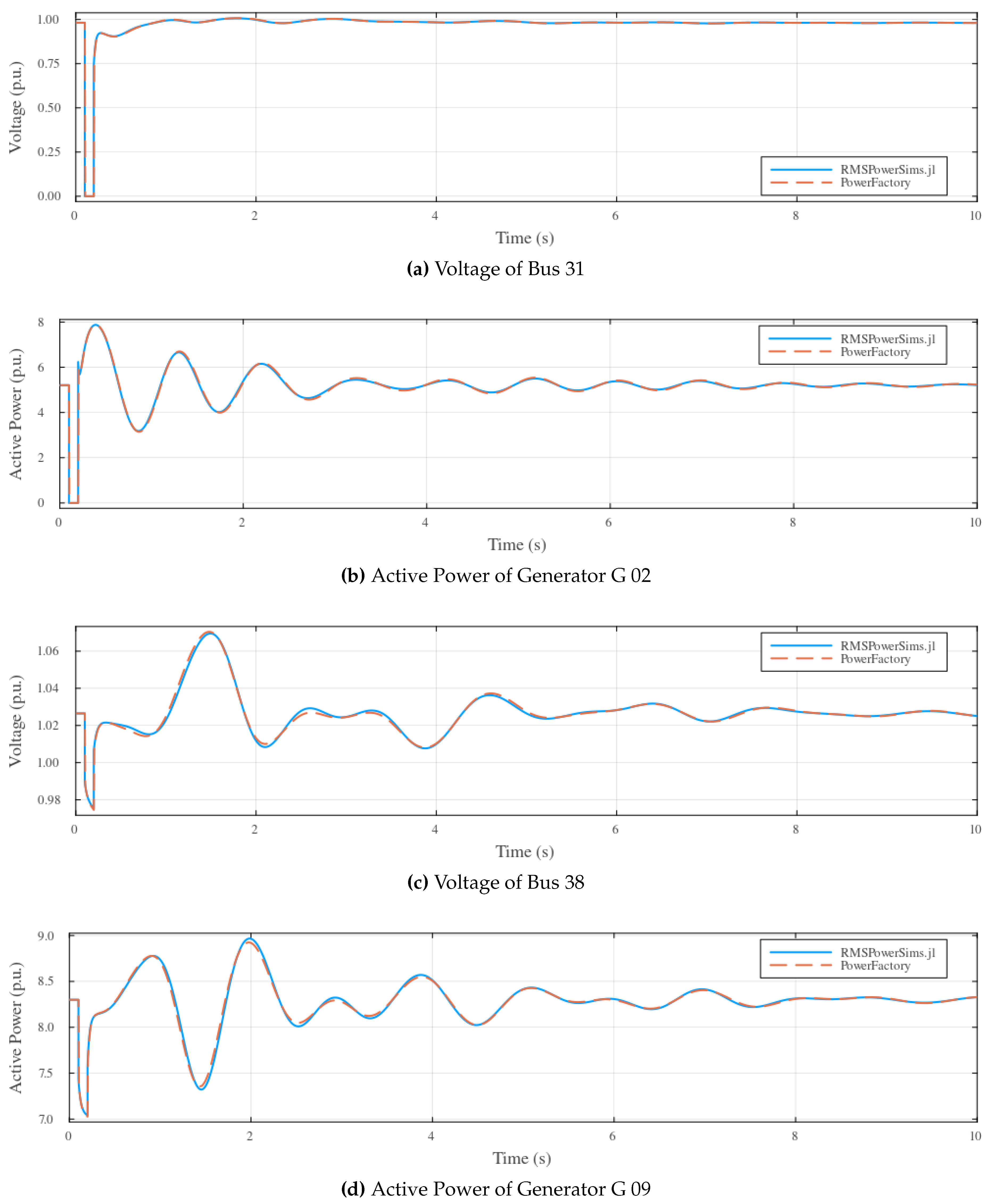
The results discussed in this section relate to a simulation in which a bolted short-circuit fault occurs at Bus 31 at , and is cleared at . RMSPowerSims.jl is set to recalculate the state of the system both at the time of the fault, and at the time of clearance. Figure 4 shows comparisons of the time series results produced by RMSPowerSims.jl and PowerFactory. As can be seen in Figure 4(a) and Figure 4(b), both the voltage at the faulted bus and the active power response of the generator connected to faulted bus, G 02, match the results produced by PowerFactory quite closely. Figure 4(c) and Figure 4(d) show the voltage of Bus 9 and the active power response of the generator connected to Bus 38, G 09, which is distant from the fault. The results here are also shown to be in close agreement with those produced by PowerFactory.
It is worth noting that while the verification processes of other software packages commonly use metrics such as the root-mean-square error of the compared signals, we have simply opted for visual inspection in this case. The reasoning for this is that the synchronous generator models used in RMSPowerSims.jl and PowerFactory are not strictly identical [29], and as such, the results produced by the two packages are not expected to match identically. Any metric based comparison would, therefore, be misleading as it is not possible to attribute which differences are due to the generator model differences, and which are the implementation of the simulation package.
5. Conclusions
This paper has presented an RMS simulation capable Julia package, that is intended to be compatible with the PowerModels.jl ecosystem. The overall structure of the package has been discussed, as well as a brief overview of the simulation process. A verification process has been performed using the 39 Bus New England System to compare the responses acquired using the developed RMSPowerSims.jl pachage and DIgSILENT PowerFactory. The results clearly indicate that RMSPowerSims.jl is capable of producing accurate time-domain simulation results.
The immediate future work for the package includes the implementation of additional synchronous generator control models and renewable energy generation models. This will increase the range of systems that can be simulated and facilitate studies of modern power systems for all the researchers.
Author Contributions
Conceptualization, T.P.; methodology, T.P.; software, T.P.; validation, T.P.; formal analysis, T.P.; investigation, T.P.; resources, A.P.A, T.B. and K.M.M.; data curation, T.P.; writing—original draft preparation, T.P.; writing—review and editing, T.P., A.P.A, T.B. and K.M.M.; visualization, T.P.; supervision, A.P.A, T.B. and K.M.M.; project administration, T.P, A.P.A, T.B. and K.M.M.. All authors have read and agreed to the published version of the manuscript.
Funding
This research was funded by the Australian Government Research Training Program Scholarship and the Commonwealth Scientific and Industrial Research Organisation (CSIRO).
Data Availability Statement
The original data presented in the study are openly available in RMSPowerSims.jl at https://github.com/tphilpott2/RMSPowerSims.jl.
Conflicts of Interest
The authors declare no conflicts of interest.
Abbreviations
The following abbreviations are used in this manuscript:
| AC | Alternating Current |
| AVR | Automatic Voltage Regulator |
| DAE | Differential-Algebraic Equation |
| EMT | Electromagnetic Transient |
| IBG | Inverter-Based Generation |
| NDD | Network Data Dictionary |
| OPF | Optimal Power Flow |
| REG | Renewable Energy Generation |
| RMS | Root Mean Square |
References
- Renewable Integration Study Stage 1. Report, Australian Energy Market Operator, 2020.
- Hatziargyriou, N.; Milanovic, J.; Rahmann, C.; Ajjarapu, V.; Canizares, C.; Erlich, I.; Hill, D.; Hiskens, I.; Kamwa, I.; Pal, B.; Pourbeik, P.; Sanchez-Gasca, J.; Stankovic, A.; Van Cutsem, T.; Vittal, V.; Vournas, C. Definition and Classification of Power System Stability - Revisited & Extended. IEEE transactions on power systems 2021, 36, 3271–3281. [Google Scholar]
- Capitanescu, F. Critical review of recent advances and further developments needed in AC optimal power flow. Electric power systems research 2016, 136, 57–68. [Google Scholar] [CrossRef]
- Roald, L.; Andersson, G. Chance-Constrained AC Optimal Power Flow: Reformulations and Efficient Algorithms. IEEE transactions on power systems 2018, 33, 2906–2918. [Google Scholar] [CrossRef]
- DIgSILENT PowerFactory Website. Available online: https://www.digsilent.de/en/powerfactory.html (accessed on 18 August 2024).
- PSS/E Website. Available online: https://www.siemens.com/global/en/products/energy/grid-software/planning/pss-software/pss-e.html (accessed on 18 August 2024).
- PSCAD PowerFactory Website. Available online: https://www.pscad.com/ (accessed on 18 August 2024).
- A Review of Power System Modelling Platforms and Capabilities. Report, The Institution of Engineering and Technology, 2015.
- Lara, J.D.; Barrows, C.; Thom, D.; Krishnamurthy, D.; Callaway, D. PowerSystems.jl — A power system data management package for large scale modeling. SoftwareX 2021, 15, 100747. [Google Scholar] [CrossRef]
- NREL-Sienna. PowerSimulations.jl. Available online: https://github.com/NREL-Sienna/PowerSimulations.jl (accessed on 18 August 2024).
- Lara, J.D.; Henriquez-Auba, R.; Bossart, M.; Callaway, D.S.; Barrows, C. PowerSimulationsDynamics.jl – An Open Source Modeling Package for Modern Power Systems with Inverter-Based Resources. arXiv (Cornell University) 2024. [Google Scholar] [CrossRef]
- Plietzsch, A.; Kogler, R.; Auer, S.; Merino, J.; Gil-de Muro, A.; Liße, J.; Vogel, C.; Hellmann, F. PowerDynamics.jl–An experimentally validated open-source package for the dynamical analysis of power grids. SoftwareX 2022, 17, 100861. [Google Scholar] [CrossRef]
- Coffrin, C.; Russell, B.; Sundar, K.; Ng, Y.; Lubin, M. PowerModels.jl: An Open-Source Framework for Exploring Power Flow Formulations. arXiv (Cornell University) 2018. [Google Scholar] [CrossRef]
- Heidari, R.; Amos, M.; Geth, F. An Open Optimal Power Flow Model for the Australian National Electricity Market. 2023. [Google Scholar] [CrossRef]
- Philpott, T.; Agalgaonkar, A.P.; Muttaqi, K.M.; Brinsmead, T.; Ergun, H. Development of High Renewable Penetration Test Cases for Dynamic Network Simulations using a Synthetic Model of South-East Australia. 2023 IEEE International Conference on Energy Technologies for Future Grids (ETFG), pp. 1–6. [CrossRef]
- Zimmerman, R.D.; Murillo-Sánchez, C.E.; Thomas, R.J. MATPOWER: Steady-State Operations, Planning, and Analysis Tools for Power Systems Research and Education. IEEE transactions on power systems 2011, 26, 12–19. [Google Scholar] [CrossRef]
- Athay, T.; Podmore, R.; Virmani, S. A Practical Method for the Direct Analysis of Transient Stability. IEEE transactions on power apparatus and systems 1979, PAS-98, 573–584. [Google Scholar] [CrossRef]
- RMSPowerSims.jl. Available online: https://github.com/tphilpott2/RMSPowerSims.jl (accessed on 18 August 2024).
- Christopher, R.; Qing, N. DifferentialEquations.jl – A Performant and Feature-Rich Ecosystem for Solving Differential Equations in Julia. Journal of open research software 2017, 5. [Google Scholar] [CrossRef]
- Julia Documentation, Methods. Available online: https://docs.julialang.org/en/v1/manual/methods/ (accessed on 18 August 2024).
- Sauer, P.W.; Pai, M.A. Power System Dynamics and Stability; Prentice Hall, 1998. [Google Scholar]
- Exciter IEEET1. Available online: https://www.powerworld.com/WebHelp/Content/TransientModels_HTML/Exciter%20IEEET1.htm (accessed on 18 August 2024).
- Governor TGOV1 and TGOV1D. Available online: https://www.powerworld.com/WebHelp/Content/TransientModels_HTML/Governor%20TGOV1%20and%20TGOV1D.htm (accessed on 18 August 2024).
- IEEE Standard 1110-2002 (Revision of IEEE Std 1110-1992); IEEE Guide for Synchronous Generator Modeling Practices and Applications in Power System Stability Analyses. 2002.
- NLsolve.jl. Available online: https://github.com/JuliaNLSolvers/NLsolve.jl (accessed on 18 August 2024).
- Christ, S.; Schwabeneder, D.; Rackauckas, C.; Borregaard, M.K.; Breloff, T. Plots.jl – a user extendable plotting API for the julia programming language. 2023. [Google Scholar] [CrossRef]
- DIgSILENT GmbH. 39 Bus New England System, DIgSILENT PowerFactory, 2020.
- DIgSILENT GmbH. PowerFactory 2022, Technical Reference, Synchronous Machine, 2022.
- Canay, I.M. Causes of Discrepancies on Calculation of Rotor Quantities and Exact Equivalent Diagrams of the Synchronous Machine. IEEE transactions on power apparatus and systems 1969, PAS-88, 1114–1120. [Google Scholar] [CrossRef]
Figure 1.
Intended procedure for running a simulation using RMSPowerSims.jl.
Figure 2.
Structure of component model types in RMSPowerSims.jl.
Figure 3.
Network diagram of the 39 Bus New England System.
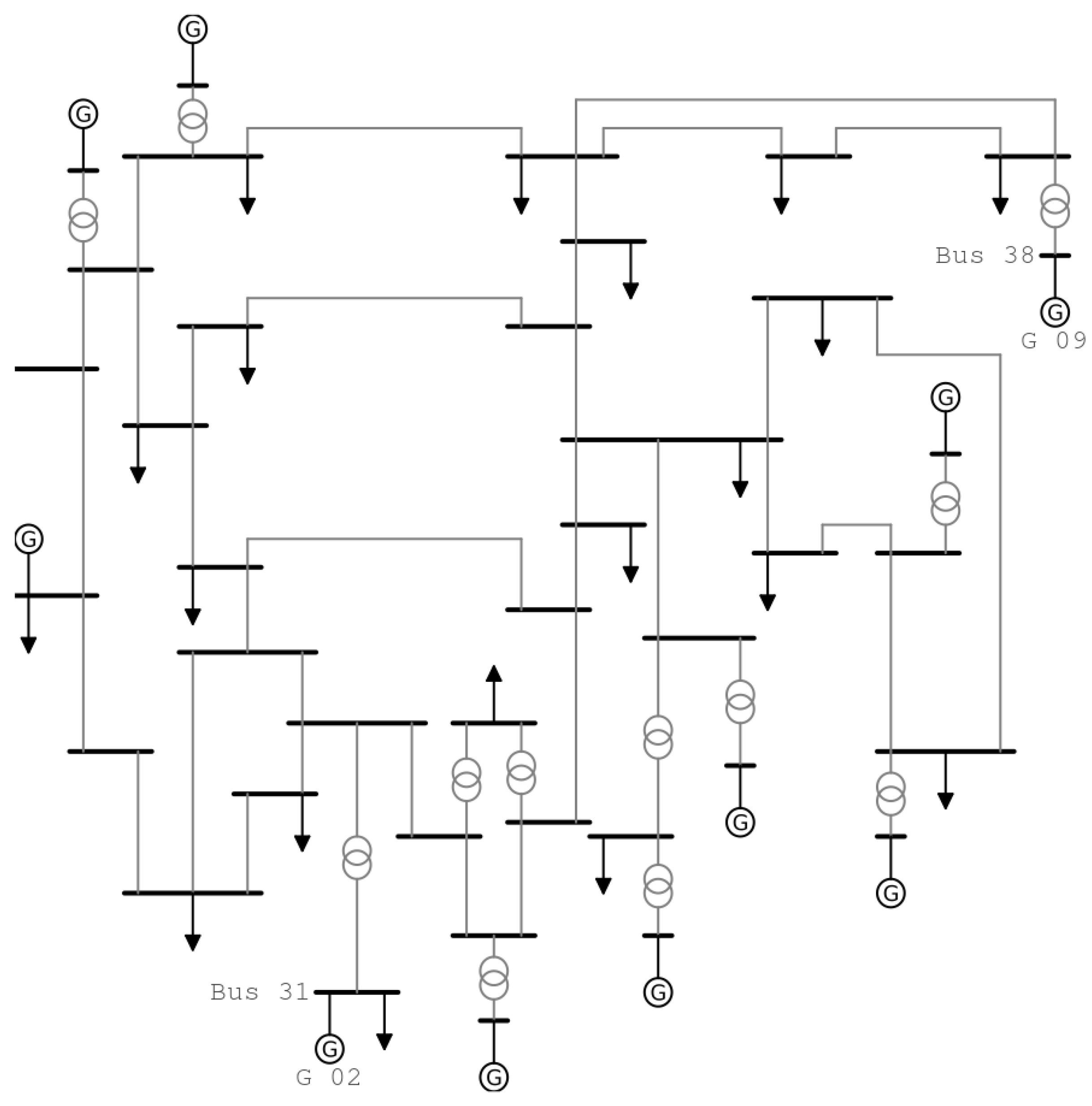
Figure 4.
Time series results for short circuit simulation.
Disclaimer/Publisher’s Note: The statements, opinions and data contained in all publications are solely those of the individual author(s) and contributor(s) and not of MDPI and/or the editor(s). MDPI and/or the editor(s) disclaim responsibility for any injury to people or property resulting from any ideas, methods, instructions or products referred to in the content. |
© 2024 by the authors. Licensee MDPI, Basel, Switzerland. This article is an open access article distributed under the terms and conditions of the Creative Commons Attribution (CC BY) license (http://creativecommons.org/licenses/by/4.0/).
Copyright: This open access article is published under a Creative Commons CC BY 4.0 license, which permit the free download, distribution, and reuse, provided that the author and preprint are cited in any reuse.


