1. Introduction
Magnetic hysteresis is a fundamental phenomenon in electromagnetism describing the nonlinear behavior of ferromagnetic materials [
1,
2,
3]. There are several mathematical models to represent the trend. The Jiles-Atherton model [
4,
5,
6,
7], e.g., describes the phenomenon using a physical approach based on energy considerations and magnetization theory. It is particularly known for its ability to model real magnetic materials with good precision, when there is no significant complexity in the hysteresis processes. The Stoner-Wohlfarth model [
8,
9] describes hysteretic behavior in ferromagnetic nanoparticles and granules. It assumes that magnetization rotates consistently within a particle, making it particularly useful for small systems. The Prandtl-Ishlinskii model [
10,
11] is also used for other types of hysteresis besides magnetic ones. It is known for its simplicity and ability to model rate-independent hysteresis. Many other models can be mentioned, such as those of Krasonsel’skii-Pokrovskii, Maxwell, Bouc-Wen, Dahl and so on [
12] but of all, certainly, the most used is the Preisach model (PM) [
9,
13,
14] which represents one of the most effective methods of describing hysteresis, using an overlap of elementary operators to capture the complexity of such phenomena. Since its initial formulation, various models have been developed to include other particular characteristics of the process under analysis. We mention only some of the most relevant: 1) Non-linear Generalized PM (GNP) [
9,
12,
15,
16,
17] allows hysteresis to be described more flexibly, being more accurate even when considering magnetic materials whose non-linear properties do not satisfy the classic PM; 2) Time-dependent PM [
9,
15,
18] which, by introducing the temporal dependence, allows to describe phenomena of dynamic hysteresis, where the system response depends on the rate of change of the applied field; 3) Stochastic PM [
9,
19,
20], which includes random elements to represent uncertainty and variability in materials. This extension is useful for modeling systems in which magnetic behavior presents intrinsic noise or variability due to factors such as material imperfections, thermal fluctuations or other forms of stochastic disturbances; 4) PM with limited memory [
9,
20,
21], where only part of the past history affects the current state of the system. This approach is particularly relevant for systems with short-term memory; 5) Inverse PM [
15,
19] is used to identify material characteristics from system response measurements. This approach is useful for the characterization and experimental analysis of materials; 6) Vectorial PM [
22,
23] extends the original model to include vector dependence, allowing to describe three-dimensional systems and their response to magnetic fields applied in different directions; 7) PM with Interaction between Hysteron [
24,
25,
27]. This extension introduces the interaction between hysteron, making the model more realistic for materials in which the elementary units of hysteresis are not independent but affect each other’s response
1.1. Artificial Neural Network Architectures
As in many other fields of pure and applied sciences, the use of the Deep Learning (DL) Neural Networks (NN) is beneficial for the phenomenon of magnetic hysteresis as well. In recent years, applications of artificial neural networks (ANN) to hysteresis models (basic or generalized that are) has shown considerable potential in improving the accuracy and efficiency of modeling [
5,
22,
24,
25,
26,
27,
28,
29,
30,
31,
32,
33,
34,
35,
36]. Neural architectures can obviously be of various types, depending on the specifics of the problem to be treated and the objectives that are proposed, but the common result is always to have a substantial gain in terms of computational costs or memory allocation. Sometimes this can be at the cost of better results in terms of accuracy or error than traditional methods [
24]. To cope with this, we also resort to hybrid forms of ANN or combined forms of ANN and traditional models of hysteresis, as in the examples we will see below. In any case, assessments must of course be made on a case-by-case basis.
In the following sections we will show just a few of the several possible ANN, based on the results obtained in the literature and comparing the advantages or limitations of the various approaches. In particular, we are going to examine the use of Feedforward neural networks (FNN) and Recurrent neural networks (RNN) in the context of modelling magnetic hysteresis by using the Preisach model. We will analyze the effectiveness of each type of network in predicting hysteretic behavior, comparing their performance in terms of accuracy, convergence rate and generalization ability. The results show that the integration of neural networks with the Preisach model not only improves the representation of hysteresis, but also offers new perspectives for the analysis and prediction of the behavior of magnetic materials. In the last part of the article, we will cite a list of additional architectures used, summarizing the salient points. Our research highlights the importance of choosing the appropriate neural architecture for specific hysteresis applications, providing guidelines for future studies and practical applications.
2. Feedforward Neural Network
The first article that we will take into consideration [
28] treats the usage of ANN to implement the Preisach model for the modeling of magnetic cores. Traditionally this process requires complex and computationally expensive mathematical models. The authors propose instead to use the ANN to create a more flexible and adaptable model as useful to simulate complex multi-variable and time-dependent processes. Like other neural networks, they can be used for specific cases as well as for general descriptions being able to predict even random behaviors of the system as well as to respond to inputs not belonging to the initial datasets. In FNN, among the most common NNs, information moves in one only direction, from the input to the output phase, without cycles or loops. The goal of the authors is that the network learns the complex relationship between the applied magnetic field
H and the consequent magnetic induction
B in the material. Once trained, neural networks are able to predict the behavior of the magnetic hysteresis cycle for different operating conditions without the need for detailed mathematical models. This approach offers a more efficient and flexible alternative to traditional methods.
A hysteresis function represents the input/output connections with multi-branch non-linearities, where the turning points of the hysteresis branches are affected by the past minimum/maximum input values [
1]. Such definition outlines a key property of the hysteresis phenomenon, namely a sequential behavior in which the output must be determined depending of both input and internal states. PM can be used as a mathematical tool to describe this process [
14] and can be built as follows.
Definition 1 (Preisach Model).
Let input , output can be uniquely determined
where , are the switching values up and down input, the finite set of binary hysteresis operators useful as local memory, the hysterons distribution (model coefficients by experimental data).
Among the FNN, in particular the authors in [
28] use the Radial Basis Function NN (RBF-NN), employed for classification, approximation problems and strict interpolation in multidimensional space [
37,
38,
39,
40]. They are preferred over multi-layer perceptron (MLP) because they are faster in the learning phase. This is due to the fact that this type of architecture does not require multi-layers but only one layer that includes the RBF, each of which depends on the respective centers
c and amplitude
r. The number of centers (and therefore of respective connected neurons) can be high and the choice random and this would imply high computational complexity and cause a numerical ill-conditioning. To avoid this, the type of RBF and the type of centers should be carefully chosen. They are usually chosen from the points of the dataset(
) but this does not guarantee a complete mapping of the sample, instead the approach used in [
40], based on Orthogonal Least Square (OLS) method ensures better performance and the ability of the network to achieve the results of a MLP despite its two layers. The technique is based on the fact that RBFs are seen as special cases of a regression model
where
is the desired output,
are the parameters,
the so-called regressors (fixed functions of the input
) and
the error assumed uncorreleated with
. Through this formulation, in our context, a fixed center
with a non-linear activation function
corresponds to a regressor
and the problem of how to select a appropriate set of RBF centers corresponds to the selection of considerable regressors from a given candidate set (OLS method). The iteration ends at step
, with
is a chosen tolerance. In
Figure 1 a comparison between a classical MLP scheme and a RBF scheme.
Despite having a similar structure composed of input, hidden and output layers, the activation functions are then radial basis and therefore typically Gaussian, Spline, Multi-Quadratic or Multi-Quadratic inverse, instead of typically sigmoid. The included two parameters,
c and
r, associated with RBF neurons, are similar to hidden layer weights and biases in MLP. Finally, the output returns a weighted sum of its inputs using the appropriate weights
. The network training consists largely in what has been illustrated so far, namely finding an adequate number of these parameters and associated neurons and calculating their weights through various algorithms. The OLS method to minimize the errors between the desired output and that predicted by the neural network is used by the authors in [
28]. The expression for the processing of the input through function of activation and the restitution of the relative outputs has the standard form for the neural nets
where
activation function, in this case of Gaussian type,
weights. The correspondence with the Eq. (
2) is evident. At this point, reconstruction of the Preisach model is obtained by using normalized hysteresis cycles data for the square Permalloy 80 at various frequencies.
NN efficiency criteria are usually based on number of epochs, training time, network size, dataset, loss function and accuracy. For hysteresis modelling, the major criterium of interest is the
accuracy. In [
28], comparisons are made between experimental data and network output. To measure the error index, the Mean Square Error (MSE) of the normalized hysteresis modelling from the standard deviation of the experimental data (also called nondimensional index error (NDIE)) was used. Error indices vary from
to
with an average NDIE of
1.
3. Hybrid Architectures—FNN and RNN
Also in [
24,
25,
27], authors use FNN and PM to simulate hysteresis cycles in different materials, as well as hybrid models that will be discussed below
2. In particular, in [
24] soft ferromagnetic materials (commercial iron-silicon NGO), subjected to sinusoidal and non sinusoidal magnetic induction waveforms, are considered. The latter can lead stonglyly distorted hysteresis cycles and, therefore, the design of the relative devices can be difficult. The proper selection of materials to be used for specific applications can be finalized using proper tools. Typically, designers rely on Finite Element Method (FEM) approaches, which are able to provide reliable predictions of the material performances when they work under given working conditions. In this analysis, the authors use PM to generate a larger dataset consisting of a family of first order inversion curves (FORCs), suitable for NN training. The hysteresis model thus generated has the ability to also detect sub-loops in the cycles. The comparison between PM and NN has been extended also to other measurements, in particular several hysteresis cycles, taken for different kinds of excitation, have been considered. Also in these cases, NN performed surprisingly good from computational efforts and memory request sides. It should also be noted that the proposed method allows the reversal of the problem (
) and therefore the comparison with the FEM (open problem). In the article, a first overview of the hysteresis models usually used is also proposed. In addition to the PM then used for comparisons, the play model, stop model and those derived from Stoner and Wohlfarth are also considered, all very accurate but computationally expensive models. Conversely, models such as the Jiles-Atherton are inexpensive but not as accurate. Unlike what is shown in [
28], the optimization model for the output layer of the FNN used in [
27] is the Levenberg-Marquardt algorithm [
41]. The FNN thus obtained are usable for sinusoidal magnetization processes as well as other kinds of waveforms, with the limitation related to the impossibility about the reproduction of sub-loops, for which a technique called "transplantation" [
42] has been considered. As explained in [
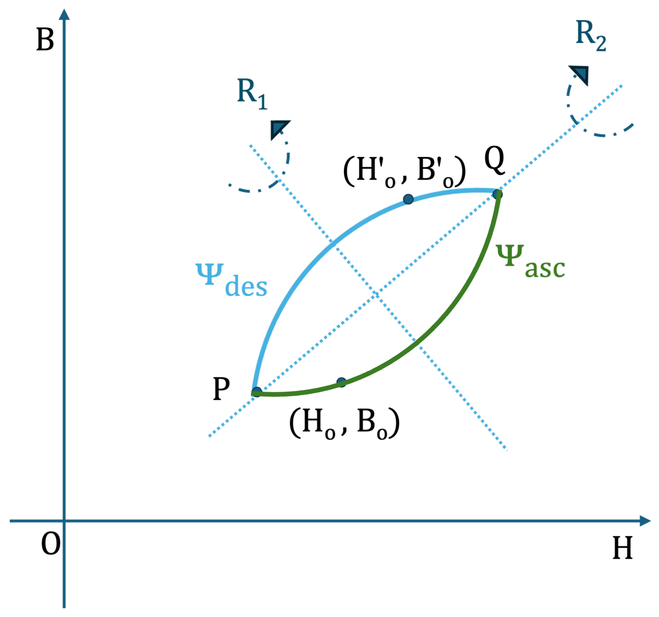
43], this algorithm is able to close a sub-loop operating a transplantation of the points in one branch of the sub-loop. An example is provided in
Figure 2, where the blue branch is obtained from the corresponding points in the green branch.
To conclude, approaches based on NN are able to recognize and associate the proper hysteresis cycle to the specific analysed sample.
Considering therefore the PM, there is the possibility to derive an analytical expression for the Preisach distribution by solving the Everett integral
3 [
9,
44] while, numerically, through various numerical methods ([
45,
46]) or approximating with suitable probability density functions. To reduce the number of parameters required by the model, in [
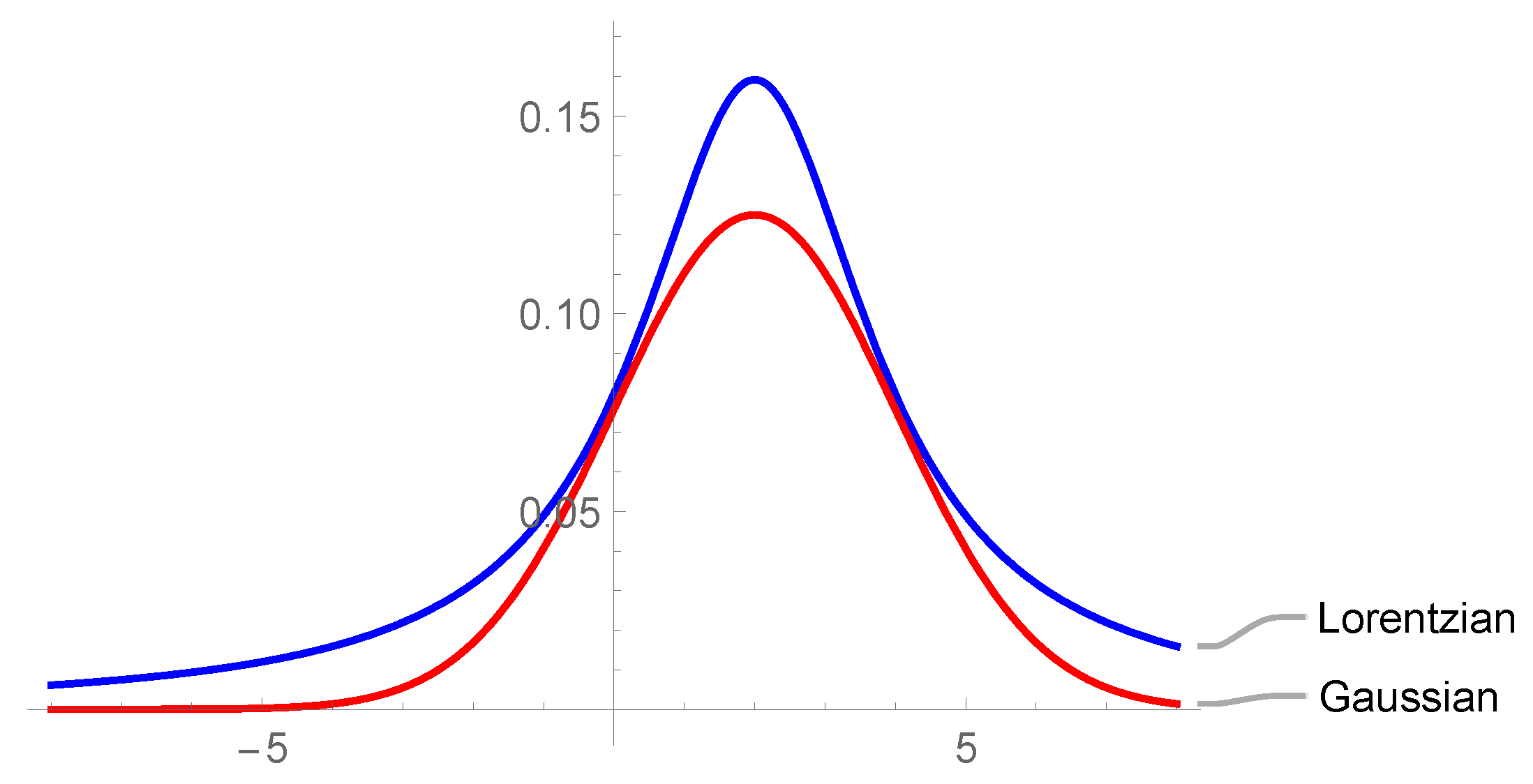
24] a formulation related to the Lorentzian probability density function approximation has been proposed (in
Figure 3 Gauss and Lorentz distributions are compared. The latter was chosen because of its slower diffusion).
The couple
(interaction field and coercive field respectively), identifies the hysterons, which must be distributed in relation to both. The distribution function
can be written by using the principle of variables separation, so obtaining
with
parameters of control of emissions
and
u,
the most likely coercive field of hysteron (related to the material coercive field). An optimized array, structured according specific rules, drives the disposition of hysterons on magnetic field axis and their corresponding
u values. The main problem related to this model is that many hysterons are required to reliably predict the hysteresis loops (
). Eq. (
4) allows instead to reduce the parameters of the model to only three (
). Another important advantage is that, using proper algorithms, there is the possibility to identify the model parameters with a reduced number of measurements (just a limited amount of hysteresis loops is required). In the work, in particular, the authors use 4 cycles of sinusoidal hysteresis for the identification of the PM. The error function
which must be minimized consists of 3 contributions:
MSE error, normalized sample by sample, evaluated considering measured and calculated
B values of the main cycle (
), with
,
where
is the
element of the
sequence of measured and evaluated
B fields.
The second term is the normalized MSE of the error between the measured value maximum and calculated value of the magnetic induction in the vertices of the cycles.
The last term is introduced to improve the accuracy of the model by introducing cycle areas for the calculation of hysteresis losses
with
areas of
calculated and measured hysteresis cycles.
The calculation of the distribution of hysteron can have in general more solutions consists of two stages. Many hours are requested for the first one, since lots of parameter combinations need to evaluated with a cost function. Anyway, using the previously defined function, the probability of obtaining a local minimum cost function is significantly reduced, thus accelerating the next step that involves the optimization algorithm. The identification procedure is quite expensive from computational point of view, especially if
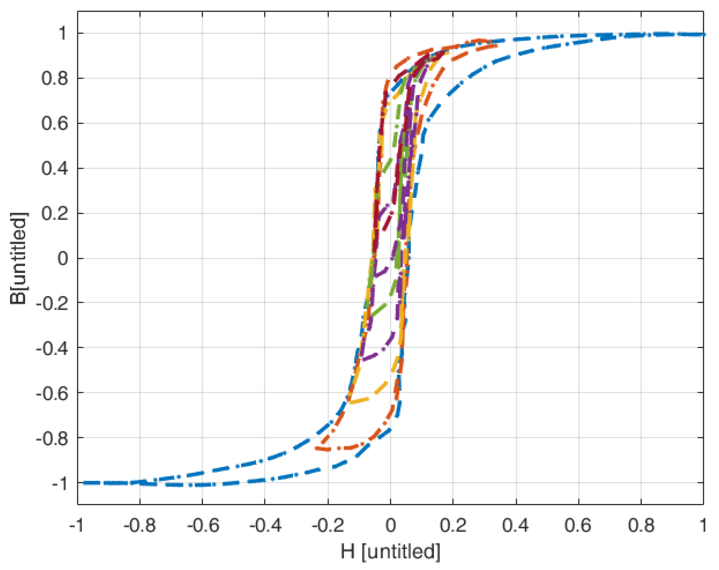
is great, however it must be considered for each material. In
Figure 4 the family of the 20 normalized FORC considered for the training of NN has been reported.
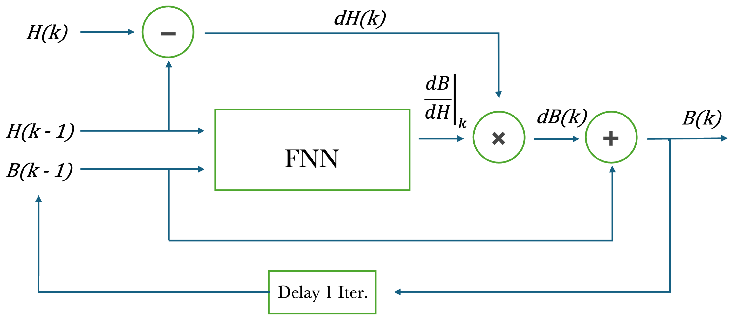
The hysteresis model based on NN is divided into two steps: firstly, the development of a standard FNN able to reproduce the natural memory of magnetic hysteresis, but characterized by a limit in the reproduction of hysteresis loops. Secondly, the usage of specific approaches to stabilize the magnetic accommodation, with the consequent advantage of accurately reproduce the sub-loops. In this way, the resulting model considerably gained more generality, with the possibility to be applied for a large variety of cases. Basically, the model is built as an FNN (structured with two hidden layers each containing 7 neurons (see
Figure 5)) which take in input the magnetic field and the magnetic induction at the instant
, and provides as output the differential permeability at the
k instant. A sigmoid activation function (or hyperbolic tangent) is applied to the hidden layers’ neurons, and a linear transfer function is applied to the output layer. Hyperparameters have been experimentally optimized. From the diagram, it is possible to see that the insertion properties of past data are included in the last step, this process is not intrinsically included in the FNN. The value of the magnetic induction at the
k instant is evaluated as
. As stated in the previous lines, the FNN provides the value of the differential permeability at the
k instant (
). The differential increment of the magnetic field (
) can be easily obtained using the previous and the actual value of the magnetic field. Finally,
. Weights (70), neuron biases (15) and training set (the family of 20
Figure 4) are the only elements influencing the net, which is identified only once for each material. The maximum number of epochs considered is
, while performance evaluation is based on MSE. The network was trained six times and its robustness was tested each time simulating 20 FORC, derived as under sampling (with a factor 8) of those applied for training. This procedure was adopted to avoid local minima of MSE, which could be found as consequence of the training set identification. The best NN obtained a
. The entire procedure was completed within 30 minutes.
If the input CM is characterized by oscillations between and (two chosen ends), and the neural network starts from an arbitrary magnetized state, several periods will be necessary to reach a stable magnetization cycle. This feature is called ’accommodation’, and it is typical just of some kinds of materials. For example, it does not affect electrical steel, where sub loops are practically stable and a simple neural system is sufficient, but where present, requires a high numerical cost. The network used offers a considerable computational advantage thanks to the previously mentioned transplantation technique. Ultimately, PM was used to create a FORC dataset to be used as a dataset for the neural network and it has been proven that the implemented neural model has been able to replicate the behavior of PM asking for lower computation effort and reduced memory storage request.
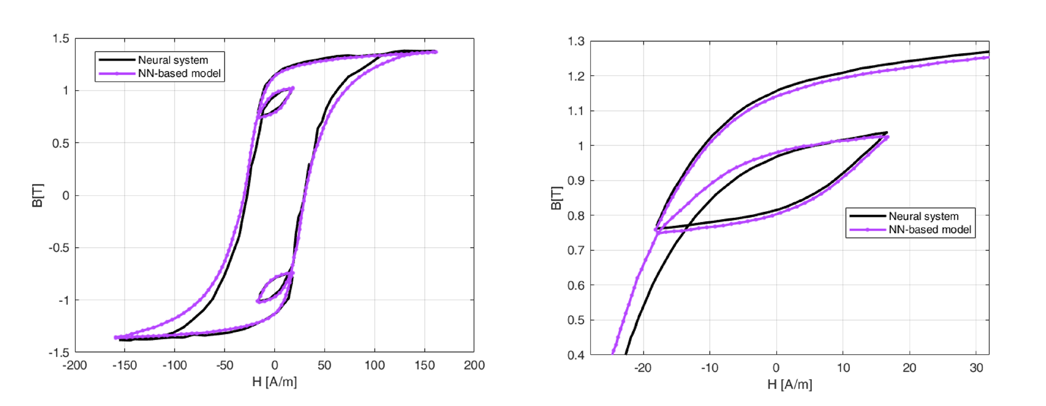
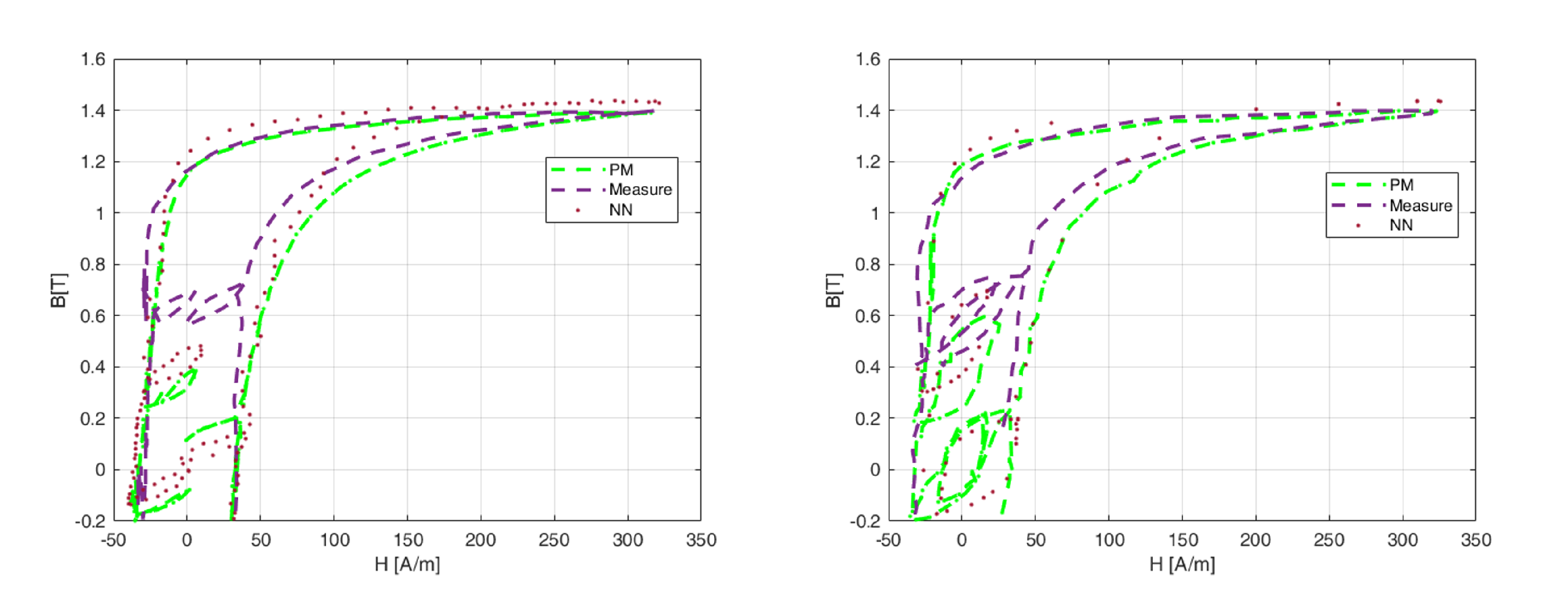
Figure 6 shows the predictions of hysteresis loops, including short loops evaluated with the transplantation technique, comparing a NN-based model and a neural system alone. Different sets of experiment data have been used for similations. Computations and experiments have been showed in
Figure 7, considering the hysteresis cycles of one of the analysed sets. Relatively to this comparison, it is important point out that NN-based model performs worse than PM. Indeed, the maximum percentage error from the experimental reference, is
for the NN model,
for PM. The origin of this inaccuracy is mainly related to a little phase error between simulated
and the applied input magnetic field
. In fact, a phase change in the waveform of the magnetic field is enough to match experimental cycle. Anyway, the phase error is always under 10 degrees, and it can be associated (at least partially) with the accuracy in the measurement of the magnetic field. As it can be seen, an error about the positioning of the sub-loops is committed, even if the resulting area is quite similar. This is because the power losses due to hysteresis evaluated with the two models (NN and PM) agree in a quite good way with measurements. This result, together with the computational advantages, still makes the method worth considering.
Moreover, it should be noted that, since the FNN provides as output the relative differential permeability, the NN-based model can also work in a reversed way (taking B as input and giving H as output), which is exactly what FEM solvers do.
4. Further Neural Architectures
As highlighted in the introductory section, the NN can be varied and in turn combined, depending on the proposed objectives. Within the 4 macro-areas of action (Classification, Regression, Clustering and Anomaly Detection) it is possible to have supervised or unsupervised input and predictive or descriptive logic. Within these, choices of hyperparameters, hidden layers, activation functions or metrics to calculate the error, give rise to infinite possibilities, not least the additions of Reinforcement, Self-Supervised or Contrastive Learning techniques. The DL can also work in combination with the ML or, as seen in the previous sections, with known numerical methods. It is clear that they are compatible with PM, extended PM, or other models of magnetic hysteresis. It is therefore not possible to give an exhaustive framework of the possibilities, but the following is limited to listing some papers belonging to some of the main categories already mentioned.
4.1. Recurrent NN, Diagonal RNN and LSTM
Another important family of neural networks is that of aforementioned Recurring neural networks [
48]. They are designed to work with sequential or temporal data, as they contain loops that allow them to maintain information about past events. They are used when data has a temporal or sequential structure, as in the case of time series. Among these, of particular interest are the Long Short Term Memory (LSTM) (see [
49] and Refs. therein) and the Gated Recurrent Unit (GRU) [
50]. These types of architectures are designed to better manage long-term dependencies in sequential data than traditional RNNs. They are often used in applications where it is necessary to capture long-term dependencies, such as modeling complex time series. The "diagonal RNN" (dRNN) [
29] is a specific type of RNN also used for temporal sequences but, unlike this one in which each recurring unit receives in input its previous outputs and the outputs of the other recurring units in the same temporal passage, dRNN introduces a particular structure in which each recurring unit receives only in input its previous outputs, and not the outputs of the other recurring units. This means that recurring connections across time are limited to a diagonal of the connection matrix instead of involving all units. This design simplifies the network structure, reducing the number of connections needed and improving computational efficiency. They are particularly useful when the long-term relationships between distant time positions are not as relevant as short-term relationships.
An example of such a network’s application to the hysteresis process is given by [
29]. Here, too, PM is used but the authors demonstrate that the rate-independent (RI) PM is in fact a dRNN in which the activation function is binary step. The black box technique is not used but the used activation function is a manipulated tanh. It is also shown that dRNN is also a versatile rate-dependent (RD) hysteresis system under detailed conditions. Relationships are established through direction, shape, symmetry and rate-dependency of hysteresis cycles and dRNN parameters, so that the former can be interpreted through the latter. dRNN formulated in this way can also model RD hysteresis, which are more precise than simple PM and because no additional parameters and changes are introduced to the classic dRNN. The model is trained using experimental data of materials with hysterical behavior and the accuracy is assessed by comparing model predictions with experimental measurements. Training time can be reduced considerably and machine learning frameworks such as PyTorch can be used. Moreover, the method is general, unlike the various adaptations to the various types of hysteresis that are specific to each experiment. The classic NN’s are used for both RI and RD hysteresis models but generally include a single activation function (as we have seen in the previous sections e.g. sigmoid, tanh, Gaussian,...) while hysteresis is a multi-valued phenomenon. The authors, through the use of dRNNs, avoid the common use of enlargement technique of the input space (e.g. in FNN) to expand the action of the model (incorporating e.g. Preisach-type hysterons or other coupling variables, for example of historical type), and do not use RBF-type functions with multiple inputs (common to capture non-linear relationships between historical and current variables). This approach reduces computational complexity and gives to the network the ability to learn time dynamics on its own. The dRNN architecture is more effective while maintaining the possibility to model non-linear behaviors such as magnetic hysteresis.
In [
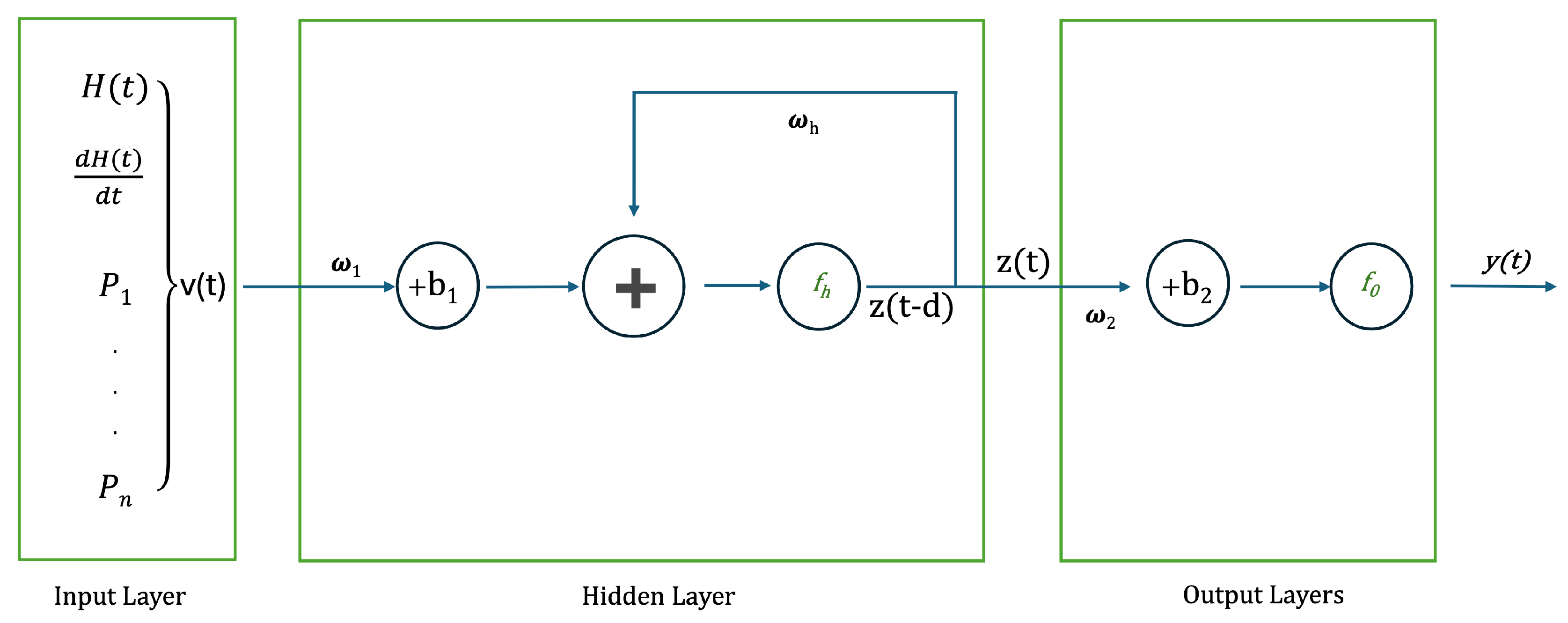
30] a Preisach-RNN model is provided to forecast the dynamic hysteresis in ARMCO pure iron, fundamental soft magnetic material used in particle accelerator magnets, without requiring prior knowledge of the material and its microstructural behavior. The dynamic aspect includes the dependence of the hysteresis cycle on the rate of change due to the interaction between electric and magnetic fields. A novel validation method is suggested to identify the model’s parameters through a RNN coupled with Preisach play operators. In general, a RNN consists, like aforementioned NN, of an input layer, a hidden layer and an output layer. Input and output layers involve feed-forward connections, hidden layer a recurrent ones. The input vector named
is processed at the input layer at each time step
t,. Later,
is summed to the bias vector
and multiplied for
, the input weight matrix. Equally, the internal state
, slowed down by a number of time instants
d, is multiplied by the gain factor
and added to the input state according to the formula
with
activation function (here tanh). The internal state
is then added with bias
, multiplied by the weight
, and the result is passed through a linear activation function
as follows
is the predicted output at time
t. The layers scheme can be seen in
Figure 8. Here, too, the Levenberg-Marquadt algorithm is used as an optimization model for the output layer. It is a non-linear least squares optimization algorithm incorporated into the backpropagation algorithm for training NN [
51]. If
is the real data, algorithm aims to optimize output through the formula
It leads to update the weights according to the following
with
represents the learning rate.
By training with only six different hysteresis loops at three frequencies, the proposed model is able to predict the magnetic flux density of ARMCO pure iron with a NRMSE better than and can predict dynamic behavior for both main and sub cycles. The model’s accuracy in predicting data that has not been measured is demonstrated through its evaluation using ramp-rates that were not utilized in the training procedure. In the field of materials science, the Preisach model, based on a RNN, has been shown to accurately describe ferromagnetic dynamic hysteresis also when trained with a limited amount of data.
In [
35], authors exhibit the ability of an LSTM network to capture the intricate hysteretic dynamics of piezoelectric actuators (PEAs). The network is established to represent the sophisticated motion of PEAs, which incorporates static hysteresis or high-order dynamics. By using data sets of input–output pairs obtained experimentally excitations of various frequencies and amplitudes, the network is trained and evaluated. Preliminary findings indicate that the LSTM network can provide adequate precision in a wide frequency range, even for the simplest topology, such as a single layer with one cell. Thus, LSTM networks may offer a novel approach to approximate the dynamics also in complex engineering systems (see [
49] for more details on LSTM scheme and mathematical model).
In [
52], ordinary differential equations are employed by the authors to model and quantify hysteresis, which is manifested in sequentiality and historical dependence. They propose a neural oscillator, "HystRNN", which is inspired by coupled-oscillatory RNN and phenomenological hysteresis models to update the hidden states (HS). The performance is measured for the purpose of predicting generalized scenarios, which involve 1
st-order reversal curves and minor loops. Results exhibit the capability of HystRNN to generalize its performance to untrained parts (essential feature for hysteresis models), as it has been discussed extensively. The paper drawing attention on the advantage of neural oscillators over the common RNN-based methods in detecting complex hysteresis patterns in magnetic materials, where traditional RD methods are not efficient to catch intrinsic non-linearities. The methology uses a structure similar to RNN with a difference included in the HS upgrade. Indeed, HystRNN apply ODEs for updating them. The procedure engages two inputs,
H and
, which are mapped to
B. The modeling process collects a number
of experimental data points and the number of training point is
. The technique shares some analogies with FNN architectures used for modeling hysteresis, but differs by including a recurrent affinity capturing longer-time dynamics and output dependencies. The cited ODE is a second-order ODE
with
denoting the HS of the HystRNN,
the time derivative,
the second-order time derivative,
and
the weights matrices.
. The aggregated training data corresponds to the time
t.
is the input,
the bias vector,
the activation functions. The authors here introduce a reduction of the differential order by using the auxiliary variable
and obtaining the first order system
They then use an explicit scheme to discretize the system for . The output obtained is finally calculated for each recurring unit. The method is evaluated using four metrics: 1) "L2-norm", for the measure of the Euclidean distance between predicted and real values; 2) "Explained variance score" denotes prediction accuracy, catching variance proportion; 3) "Maximum error" discovers important prediction discrepancies as potential outliers; 4) "Mean absolute error" evaluates mean differences between predictions and real values for general precision.1-3-4 kind of error, together with higher explained variance, imply enhanced performance. The trained architecture is tested in two different eventualities concerning the prediction of 2 FORCs and 2 minor loops. For FORC prediction, 2 different lengths of sequence (199 and 399) are tested. For minor loops prediction, a sequence with a length of 399 each has been used. As with network learning, sequence length tests also depend on data generated by the PM to evaluate the model. HystRNN has been confirmed by predicting 1st-order reversal curves and minor loops, after training the model only with major loop data. The results emphasize the primacy of HystRNN in ably catching intricate non-linear dynamics, best performing conventional RNN architectures such as LSTM or GRU on various metrics. This result is imputable to its faculty to comprehend sequential information, historical dependencies, and hysteretic features, finally reaching generalization competences.
4.2. Convolutional NN and Temporal CNN
Convolutional neural networks (CNN) are an advanced class of artificial neural networks designed for processing and analysis of structured data in matrix form, as images, audio and video. Introduced in [
53] in the ’90s, CNN revolutionized the field of artificial vision by their ability to automatically learn relevant features from raw data. They consist of convolutional layer, the heart of the architecture, composed by several layers in which a series of filters (or kernels) is applied to the input images, generating feature maps [
49]. These filters are able to capture various local features such as edges, corners and textures, essential for understanding the image. After each convolution layer, a pooling layer (usually max pooling) reduces the spatial dimension of feature maps, keeping the most important information and reducing computational complexity. This process makes the model more robust under variations and translations of the image. Finally, fully-connected layers are composed in the same way as those in traditional NN. These layers combine the characteristics learned during the convolutions to carry out the final classification or other recognition activities [
49]. They have been successfully used in a wide range of applications, including image recognition or semantic segmentation. CNNs learn to extract features at different levels of abstraction, from edge detection to complex shapes, share weights, drastically reducing the number of parameters to learn and improving computational efficiency but require large amounts of labeled data for training effective. The training also requires a considerable computational cost or specialized hardware such as a GPU. The high flexibility of the CNN can be adapted for the analysis of multidimensional data, such as magnetic hysteresis data.
In [
32], authors analize the temperature variation modifying the magnetic behavior of ferromagnetic cores and that can have impact on the performance of electrical devices. To build a temperature-dependent hysteresis model to accurately calculate electromagnetic features, in this case , it can have a significant impact. A Temporal convolutional network (TCN) in combination with the Play operator method is developed in the paper. To introduce the temperature effect, the suggested model uses the temperature-dependent spontaneous magnetization intensity as an input. The classical Play model is history dependent and rate independent and designed for static magnetic hysteresis calculations. It can be represented by Eq. (
14) in which a series of operators are integrated under the action of a rate-independent shape function
where
is the saturation magnetic flux density and
the play operator expressed as follows
with
is the value of the previous moment. Such a rate-independent model struggles to predict the dynamic loss accurately. However, the history-dependent Play model integrated with TCN is transformed into a dynamic, rate-dependent magnetic hysteresis model. The performance indicator employed to quantify the error between the model and experimental measurements is the Normalized root mean square error (NRMSE). The process of model validation involves selecting the suitable model hyperparameters and making sure that the model is robust to new data. The Bayesian optimization algorithm is employed to optimize the hyperparameters and improve the accuracy of model training outcomes. Results exhibit that the provided model can accurately forecast the hysteresis features of materials, both under varying temperature and frequency conditions.
In [
33], the problem of how the output force of pneumatic blow-off actuators is critical for their applications is addressed. Its force control poses a great challenge due to the strong asymmetric hysteresis posed by its material’s hyperelasticity and air’s high compressibility. The author propose a hybrid model named CNN - AUPI (Amplitude-dependent Un-parallel Prandtl–Ishlinskii (PI)) based force-position hysteresis modeling method for soft actuators. AUPI is a modified model built on the traditional PI, which is a weighted superposition of the multiple play operators as illustrated in the following
A single play operator is a time-varying equation. The PI superimposed by multiple play operators can only fit symmetric hysteresis curve becuase the symmetry of the play operator. Built on PI, a UPI (Un-parallel PI) is considered to model asymmetric hysteresis. The mathematical formulation is
describing the asymmetric event of the hysteresis loop by multiplying a factor
on the falling edge of the play operator. The UPI model for the soft joint actuator accurately depicts the asymmetric hysteretic behaviour at a specific inflation pressure, but develop into unreliable at varied inflation pressures. It was incorporated that the soft joint actuator’s maximum rotation angle "A" be introduced at each inflation pressure [
58] to assure the model is able to forecast hysteresis at diverse air pressures. AUPI model includes various weighted UPI operators and the constant term
where
y is the AUPI model output and
b a constant to be identified introduced to represent the actuator hysteresis curve features at the starting point. The number of UPI operators, experimentally setted, is
and
is the density coefficient of the UPI operators.
is included ito describe a segmented form involving the loading and unloading process of the hysteresis curve, respectively. Furthermore, 2 non-linear functions frequently used in hysteresis modeling, as density coefficient functions, have been applied to AUPI. Although the AUPI model has the capability to represent the asymmetric hysteresis event and generalize the results, its fitting accuracy is not enough strong under the inflation pressure independent of the training data. For this aim and so further improve accuracy and generalization model capability, a CNN is matched. CNN mechanism obtains the general characteristics of hysteresis information, avoids overfitting and dramatically enhances the composite model’s accuracy and generalization ability. The ReLU activation function provides advantages such as fast convergence and an lack of gradient saturation or disappearance (with respect to common sigmoid and tanh functions). Since the convolution layer only draws the links between local characteristic nodes, the combination of the CNN with an AUPI model obtains the genearl relationships between individual nodes of the feature map. MAE, MSE, maximum relative error, mean output force error and R-square quality of fit are used to quantitatively describe the adventages of the models. By experimentally, it is shown that the CNN–AUPI model has brilliant hysteresis fitting for soft joint actuators, with a maximum relative error of only
and a quality of fit of more than
. Other hysteresis models such as classical PI and improved PI have been compared, and the results provide that the CNN–AUPI mode has a strong modeling accuracy and high prediction ability, so providing a encouraging method for soft actuators hysteresis modeling. Furthermore, it is generalizable and suitable to model asymmetric hysteresis for different kind of soft actuators.
4.3. Generative Adversarial Networks (GAN)
Generative neural networks as, e.g., Generative adversarial networks (GAN), are used to generate new synthetic data which follows the same distribution of input data. They are among the most intriguing ideas in computer science today. An adversarial process is employed to train two models simultaneously. A generator ("the artist") learns to create images that look real, while a discriminator ("the art critic") learns to tell real images apart from fakes [
34]. As training progresses, the generator improves its ability to create images that appear real, while the discriminator improves its ability to distinguish them. The process reaches equilibrium when the discriminator can no longer distinguish real images from fakes. This process trains the GAN to generate real images that may not be found in the original dataset. This approach can be useful to generate additional data to train NN models or to explore the hidden features of magnetic hysteresis data.
In [
59], GAN is discussed as a tool to predict magnetic field values at random points in space using point measurements. Obtaining high-resolution magnetic field measurements may be difficult or impractical, which is why this technique is particularly useful for scientific and real-world applications. The implemented GAN consists of two main neural networks: a generator, which predicts missing magnetic field values, and a critic, which calculates the statistical distance between real magnetic field distributions and generated field. The architecture is shown in
Figure 9 and consist of input, 3D magnetic field (measured in a 2D rectangular area) and output (an inter or extrapolated 3D magnetic field in this region). The fields are multiplied for a binary mask
m during the training, according to the following
4
The two-step generating process is designed in the style of residual learning [
60]
The generator network generates a coarse prediction by applying a sequence of convolutional layers on and the applied mask m. At the start, the input field is reduced to a lower resolution with an increased number of channels. This approach ensures that the same quantity of information is preserved while making successive convolutions computationally less intensive. Later, to enhance the model’s field of view and enable encoding at multiple scales, many convolutions with different scaled filters are executed on the down-sampled image. Lastly, the data is up-sampled with interpolations to the original size, providing a coarse forecasting . Another generator network takes and as input and provides in similar way to . Along with that, the magnetic field is split up into small patches of pixels in a second branch. The reconstruction is improved by calculating the corresponding importance between these patches and missing pixels. The purpose of this kind of contextual attention is to overthrow localization in convolutional layers and enhance it with a comprehensive flow of information from field pixels that are magnetically distant. Convolution and attention branch are linked before up-sampling to the original resolution. On , the losses , , , and can directly be evaluated. For the adversarial loss , we necessitate to employ a critic NN. It needs to split the critic into a global critic network to evaluate the whole image, and a local critic network to determine the quality of the filled-in regions. The model can predict missing magnetic field values by training the generator to minimize this statistical distance, as well as minimizing reconstruction and physical losses based on Maxwell’s equations. The average reconstruction error is with a consistent region of field points and when only a few spot measurements are available. These results prove that the technique can be used effectively to reconstruct missing magnetic fields and could have applications in various fields requiring measurement and the analysis of magnetic fields. This novel method is able to perform not painting tasks, where large parts of the magnetic field calculated, relative to the general measurement area, are missing. Moreover, the physics-informed learning-based method produces better performances when compared to the other common methods. Furthermore, when regions ( pixels) of measurements are given (instead of only ( pixel)), the Gaussian processes outperform the procedure, but with the inference time of magnetic field forecasting being two orders of magnitude higher. In certain applications, such as the simultaneous mapping and localization performed in robotics, the paradigm could be a compromise between accuracy and computational time. Authors suggest that it would be very attractiving to make use of the fact that closed Poisson problems could be solved from the boundary values around the missing field information. Hence, the generator neural network could be trained to predict missing field measurements from only these values in the input layer.
4.4. FNN and Extended PM
As mentioned in the introductory section, various mathematical models and their variants can be exploited to reproduce hysterical behaviour of ferromagnetic materials to be considered. Artificial neural networks as usual NN, involving time-delay, multi-layer perceptron, and RNN, sometimes are inadequate to learn entirely hysteretic behaviors. An appropriate memory to deal with hysteresis as a non-unique non-linear event [
54] is lacking. Basdn on PM and PI hysteresis models, built on hysteresis operators relay, play and stop, in [
56] authors suggested a novel NN, the Prandtl neural network (PINN). It provides only 1 hidden layer with stop neurons. It is a linear combination of many stop operators as in the PI model. The model can be applicable to the hysteresis following Masing rules [
55]. In [
57], the same authors extended PINN by inserting an extra hidden layer with sigmoidal neurons to non-Masing hysteresis based on Preisach neural network (PMNN). Here, the stop neurons in the 1
st hidden layer are mapped into the output layer through a non-linear mapping by the 2
nd hidden layer, like in the PM. Further extension provide a novel hysteresis operator by putting together stop and play operators and using it in a NN called Generalized Prandtl neural network (GPINN), by which non-congruent hysteresis comportment could be mocked. Both PMNN and GPINN are diverse extensions of PNN. In [
31] these extensions are jointed into a new NN called Extended Preisach Neural Network (EPNN). Furthermore, it is improved for RD hystereses that the previous extensions lack. It includes 1 input layer, 1 output layer and 2 hidden layers. Input and output layers consist of linear neurons, the 1
st hidden layer, differently from PMNN, involve Normalized Decaying Stop (NDS) neurons, whose activation mechanism is constructed after the decaying stop processor with a unit threshold (
). This kind of operator can generate non-congruent hysteresis loops. In the input layer is included
, input data and
, rate at which
changes, in order to provide to EPNN the ability of learning RD hysteresis loops. In the 2
nd hidden layer, sigmoidal neurons have been included. They help the NN learn non-Masing and asymmetric hysteresis loops very smoothly. The envisaged technique allows the simulation of both RI and RD hysteresis with either congruent or non-congruent loops and symmetric or asymmetric loops. For the EPNN training, a novel hybridized algorithm has been adopted, built on a combination of GA and the optimization method of sub-gradient with space dilatation. By applying the proposed model to different hystereses processes, from various engineering areas, with different features, the generality of the model has been evaluated. Results indicate the success of the model in the identification of the examined hysteresis and the arrangement with experimental data.
4.5. Deep Operator Networks
Deep Operator Networks (DeepONet) [
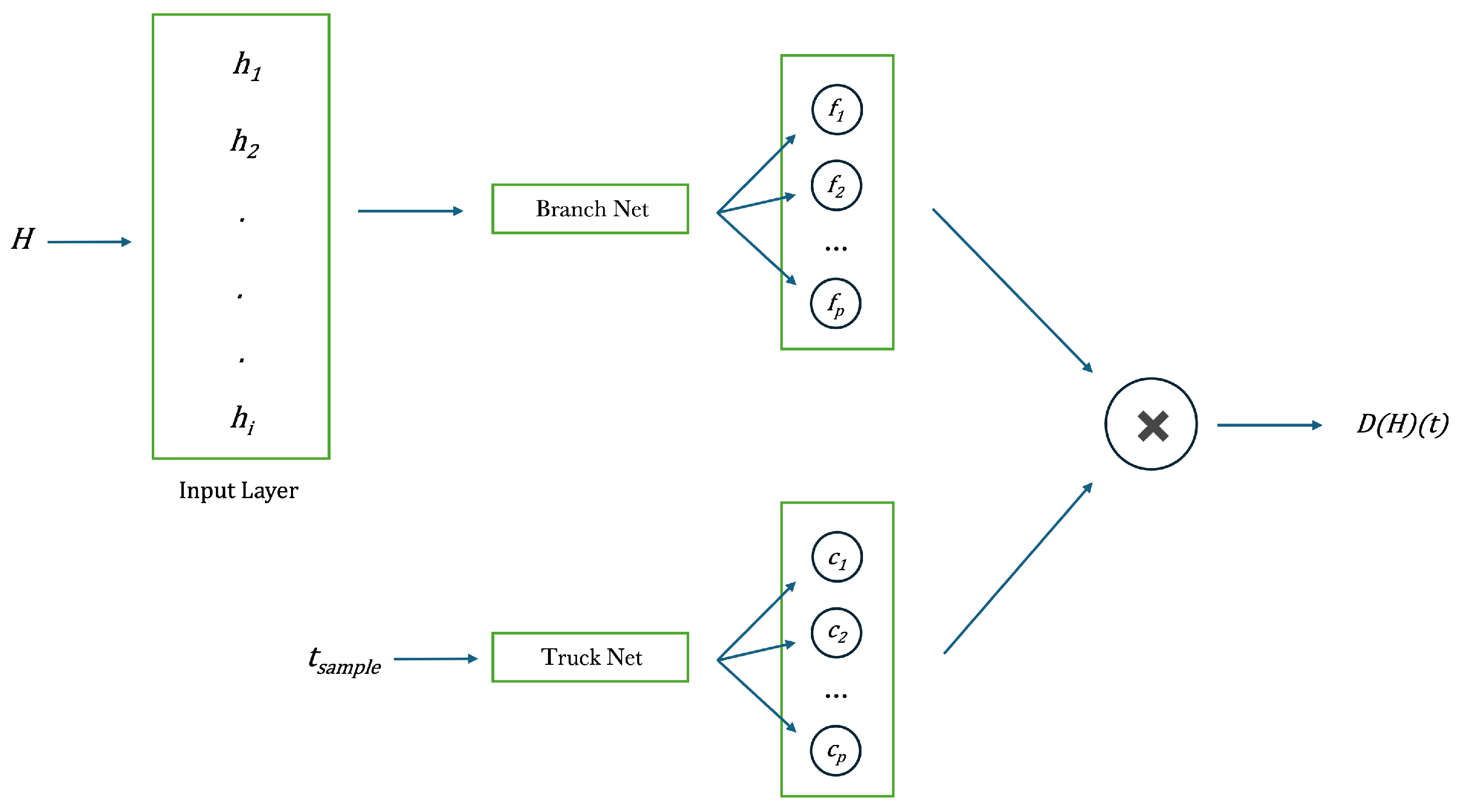
61] are a type of neural network designed to learn nonlinear operators, maps from one functional space to another. This makes them particularly suitable to model the constitutive laws governing complex phenomena such as magnetic hysteresis. In a DeepONet, the input is not a single vector as in a traditional FNN, but a function. The architecture is designed to manage these functions as inputs, so allowing to directly learn the non-linear relationships between entire functional spaces. The architecture includes 3 main sections: the Branch Network, which acquires a function as input and extracts its characteristics; the Trunk Network, captures the coordinates in the target space and transforms them into a representation that can be combined with the output of the Branch Network; the Combining Mechanism in which the output of the two networks is combined to produce the final map between the input function and the target. The structure follows a mathematical model reported in the following Theorem [
61]
Theorem 1 (Universal Approximation Theorem for Operator).
Suppose that σ is a continuous non-polynomial function, X a Banach Space, , are two compact sets in X and respectively, V is a compact set in , G is a nonlinear continuous operator, which maps V into . Then for any , exist constants , with , , , such that
This approximation theorem indicates the potential application of NN to learn non-linear operators from data, in the same way as ordinary NNs, where we learn functions from data but do not get information on how to learn efficiently. The key point is the new operator
G like a neural network, which is able to infer useful information from known and unknown data. The general accuracy of NNs can be described by separating the global error into 3 main types: approximation, optimization and generalization errors (see [
61] and Refs. therein). But, Theorem 1 guarantees a small approximation error for a adequately significant network, also if it does not consider the critical optimization and generalization errors at all, which are often preponderant contributions to the total error in effect. Useful NN should be simple to train, it means to exhibit small optimization error and generalize well to unkonwn data (namely with irrelevant generalization error). To prove the ability and effecacy of learning non-linear operators by NN, the problem is considered as general as possible by using the weakest acceptable restriction on the sensors and training dataset. The DeepONet structure makes it possible to achieve small total error and model complex processes involving whole functions, overcoming the limitations of traditional neural networks when it comes to generalizing new inputs. Applications are in several fields, including modeling of magnetic hysteresis.
The limits of traditional neural architectures, including RNN and appropriate variants (Gru, LSTM and so on), occur from their capability to learn only fixed-dimensional mappings between magnetic fields. Such networks cannot model mappings between functions in continuous domains [
62,
63]. In [
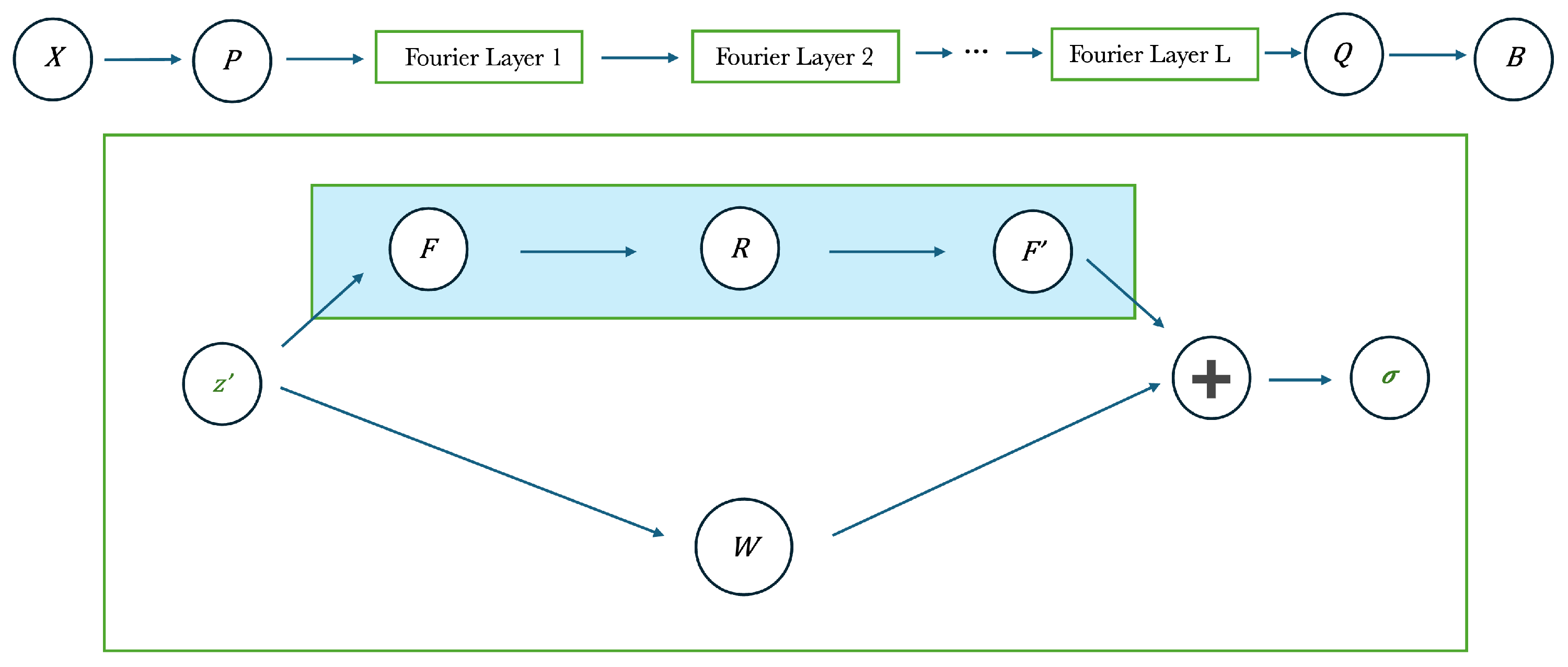
36], authors propose neural operators (NO) to model the hysteresis relationship between magnetic fields, to deal with these challenges. Common NN learn fixed-dimensional mappings, instead NO approximate the underlying operator, building a mapping between H and B fields, to predict material responses (B fields) for new H fields. Precisely, NO can approximate continuum mappings even when used on discrete data, permitting them to generalize to new H fields. More particularly, 2 notable neural operators, DeepONet and Fourier NO (see
Figure 10 and
Figure 11 and [
36] for each detail), are employed to predict new 1
st-order reversal curves and minor loops (new means they do not belong to the training dataset). Furthermore, a RI Fourier NO is proposed to forecast material responses at sampling rates diverse from those utilized during training, to incorporate the RI features of magnetic hysteresis. Numerical experiments presented demonstrated that NO adequately model magnetic hysteresis, overcoming the conventional neural recurrent techniques on different metrics and generalizing to new magnetic fields. The observations underline the benefits of using neural operators for modeling hysteresis under varying magnetic conditions, highlighting their importance in characterizing magnetic material of devices.
Author Contributions
Conceptualization: S.L., M.L., A.S. and A.F.; methodology: S.L.; data curation: S.L., G.A., E.F. and F.V.; validation: S.L., G.A., E.F., F. V., M.L., A.S., F.S., V.B., A.D. and A.F.; formal analysis: S.L., G.A., E.F. and F.V.; writing - original draft preparation: S.L.; writing - review and editing: S.L., G.A., E.F., F.V., M.L., A.S., F.S., V.B., A.D. and A.F.

