1. Introduction
In the wake of artificial intelligence development and factors such as the SARS Covid-19 pandemic, a series of changes have accelerated the transition towards a more digitalized society in many areas of daily life, particularly in those where physical presence has been found unnecessary, and where it is possible to provide quality service remotely.
This technological development has led to an increase in the number of smart devices ("wearables") and remote analysis and diagnostic methods. These are less invasive and more "comfortable" systems for the patient, which can be applied remotely, eliminating the need for an in-person consultation.
The principle underlying most remote monitoring devices is remote plethysmography. Remote plethysmography (rPPG) is a technique used in medicine to assess blood flow and vascular function in different parts of the body, especially the limbs. Plethysmography itself refers to the measurement of changes in the volume of an organ or tissue. In the specific case of monitoring devices, a light source and a sensor or photodetector are typically used to capture these changes in a specific area of the body.
Delving into the principles of video-based remote photoplethysmography, which uses a video camera as a photodetector to measure changes in blood flow in the skin, this paper aims to lay the groundwork for advancing the state of the art in this technique. It seeks to leverage the advantages offered by artificial intelligence, particularly in image and signal processing, to accurately and non-invasively measure heart rate and blood pressure from anywhere using the front camera integrated into smartphone devices. This will bring about a paradigm shift in health and wellness monitoring across all sectors of society, with benefits both economically and in terms of cardiovascular disease prevention.
2. Related Work
One of the initial articles addressing the challenge of extracting heart rate from video images recorded with a webcam is by Poh et al.[
1]. This article serves as the foundation for future work in this field. It introduces video-based remote photoplethysmography as a novel approach that can be applied to color video recordings of the human face, relying on automatic face tracking combined with Blind Source Separation (BSS) of color signals into independent components.
While Poh et al.’s work represented a breakthrough in the state of the art and laid the groundwork for all subsequent studies focused on video-based remote photoplethysmography, it also presented some limitations, particularly concerning ambient light and participants’ skin pigmentation. Consequently, some studies have explored the use of infrared and thermal cameras. Notably, within infrared cameras, S Kado et al.[
2] employed an optical sensor along with infrared and RGB cameras. The main idea of this method is to automatically select appropriate facial patches for heart rate estimation in both the spatial and spectral domains. This spatial and spectral facial patch selection allows for robust heart rate estimation in various situations, including scenarios where existing RGB camera-based methods fail to estimate heart rate accurately.
The work by Yang F et al.[
3] utilizes RGB cameras alongside thermal cameras. They propose a contactless vital signs monitoring system capable of measuring body temperature (BT), heart rate (HR), and respiratory rate (RR) using a thermal camera and an RGB camera. To achieve this, a facial detector based on convolutional neural networks (CNN) was used, and three regions of interest (ROIs) were identified based on facial landmarks for the estimation of vital signs. Heart rate is estimated using Independent Component Analysis (ICA) and a signal selection method based on Empirical Mode Decomposition (EMD).
Regarding blood pressure estimation, one of the early works laying the foundation for extracting blood pressure from video plethysmography is the study by Secerbegovic, A. et al.[
4], proposed in 2016. This study uses time-domain video plethysmography extracted from the forehead and palm of certain subjects to calculate pulse transit time, which is related to blood pressure. The forehead was selected because, according to the author, it is the region of the face that contains the strongest signal.
The aforementioned experiment was quite manual; although it defines a regression model, it is mainly based on signal processing techniques and RGB cameras. As an alternative, incorporating the use of thermal cameras, the work of Iwashita, Y et al.[
5] stands out. The objective of this study was to estimate resting blood pressure from facial thermal images. To achieve this, the components of blood pressure variations in facial thermal images were separated using Independent Component Analysis (ICA). Resting blood pressure was estimated using the independent components extracted through multiple regression analysis.
These findings were later utilized in the work of Luo, H. et al.[
6], who, using TOI (Transdermal Optical Imaging), were able to extract information from different regions of the face simultaneously, providing richer and more accurate data for blood pressure estimation than developments focusing on a single facial region, ROI, and dealing with much more homogeneous plethysmographic information. TOI technology employs advanced plethysmography techniques to extract and process plethysmographic signals. Unlike other technologies, TOI divides each video image into bit planes across the three color channels and uses a machine learning algorithm to extract hemoglobin-rich signals while eliminating melanin signals. The hemoglobin signals are combined to create a map of hemoglobin concentration on the face, generating a video that shows the oscillations of facial blood flow. This methodology offers a robust, low-noise signal, minimizing the influence of skin tone.
Similar to heart rate estimation, the estimation of blood pressure using remote photoplethysmography has also led to studies aiming to reduce the amount of signal processing techniques needed to extract vital signs, taking advantage of the benefits offered by Deep Learning and, more specifically, computer vision. In this regard, although the literature found is rather scarce, the work by Wu, Jiaze, et al.[
7] stands out. Using the PhysioNet dataset, which contains photoplethysmography (PPG) and arterial blood pressure (ABP) signals, they apply a wavelet transform to the PPG signal to draw the scalogram and use this image as input to a convolutional network to try to classify blood pressure more accurately.
3. Method
Video-based remote photoplethysmography (rPPG) analyzes and processes images or videos of human skin illuminated by ambient or dedicated light sources to recover the photoplethysmographic signal from which physiological parameters are extracted. This photoplethysmographic signal is generated from the color changes in the skin that occur due to variations in blood volume during a cardiac cycle.
When the skin is illuminated, two reflection components are generated that, although invisible to the human eye, can be captured by optical sensors like the lens of a digital camera. The first component, the diffuse reflection component, carries the PPG information as it diffuses through the skin, while the second component, the specular reflection component, is scattered across the skin’s surface. Although the specular component does not contain pulse information, the total reflected light observed by the camera depends on the relative contribution of both components.
The precise measurement of both reflection components over time generates a photoplethysmographic signal, from which vital signs such as heart rate, heart rate variability, and respiratory rate can be measured. This is the signal that over which this paper will work on will build upon. To achieve this, the following section defines a set of preprocessing techniques designed to extract this signal from video and prepare it for appropriate processing by the AI models proposed in this paper.
3.1. Preprocessing
Preprocessing encompasses the set of techniques to obtain the plethysmographic signal from the frames that make up the video sequence. This signal serves as input for models responsible for extracting heart rate and blood pressure.
The first step involves extracting the frames from the videos in the dataset. Next, face landmarks are obtained for each frame. We used the Face Landmark Detection model from MediaPipe[
8]. This model uses Convolutional Neural Networks (CNNs) to locate key facial landmarks, allowing the extraction of information from strategic regions. In this case, the right cheek is selected as the region of interest due to its lower detection error.
Once the signal is extracted, it is decomposed into RGB components, as the process for obtaining heart rate uses only the green channel, while blood pressure estimation uses all components separately.
The next step is to filter the signal, since the relevant information for obtaining heart rate and blood pressure is within a specific range of the frequency spectrum. A healthy human pulse ranges between 40 and 240 beats per minute (bpm) [
9], which, converted to seconds, corresponds to 0.67 and 4 beats per second (bps) or Hz. To restrict the information to this range, a Chebyshev Type II filter is used, as it is a low-pass filter characterized by an attenuation band with a ripple zone and a flat passband with a rapid transition. After filtering, a clean and precise signal is obtained, which is essential for the subsequent analysis and extraction of physiological parameters by the estimation models.
3.1.1. Dataset
The dataset consists of two data sets: one composed of employees from our company and the other from the UBFC-rPPG dataset [
10]. In both datasets, most participants reported being normotensive and having a heart rate within normal parameters, that is, between 60 and 100 beats per minute at rest. At the start of the study, participants completed the profile on the specially created iOS app for data collection. The following information was recorded for each participant:
Room temperature (measured with a thermometer in ºC);
Age (determined by date of birth);
Gender (female/male);
Weight (in kg);
Height (in cm);
Disposition (whether the participant is active or relaxed during the measurement);
Body Mass Index (auto-completed with weight and height).
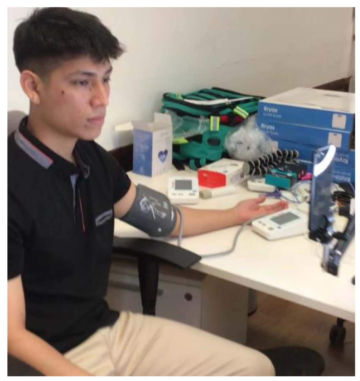
After completing these steps, participants were instructed to take a seat with their feet on the floor and position themselves in front of the tablet, ensuring that their head was centered. The next step involved placing the index finger of the right hand in a pulse oximeter to measure heart rate. A cuff was also applied for blood pressure measurement. Once both devices were properly placed, the video recording began simultaneously with the heart rate measurement. The duration of the video is approximately one minute.
Figure 1.
Recording Process Image.
Figure 1.
Recording Process Image.
3.1.2. Motion Artifacts
During the video recording, the participant is given several instructions, one of which is to remain still in front of the camera. However, small movements or changes in illumination are inevitable. These movements and changes in illumination are known as ’motion artifacts’ and can interfere with the signal of interest in the frequency spectrum. This issue is significant because heart rate is estimated specifically from the peak of highest amplitude. In the case of blood pressure, these movements can lead to errors in the selection of components during the signal segmentation process.
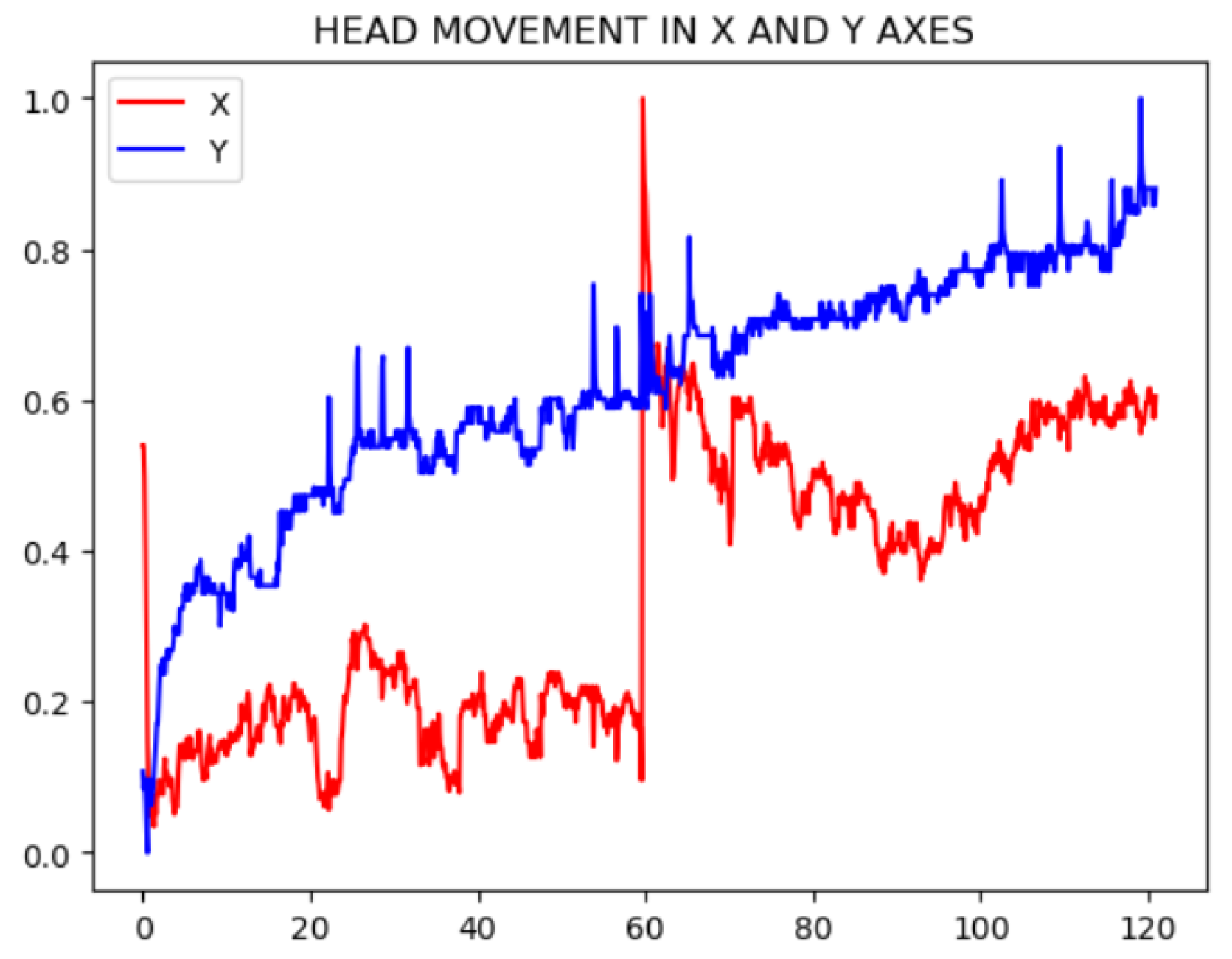
The solution developed to mitigate this disadvantage is to track the face to obtain a movement signal along the X and Y axes [
11]. This strategy involves recording the coordinates of two facial points for each frame and transforming the movement into a signal similar to the plethysmographic signal.
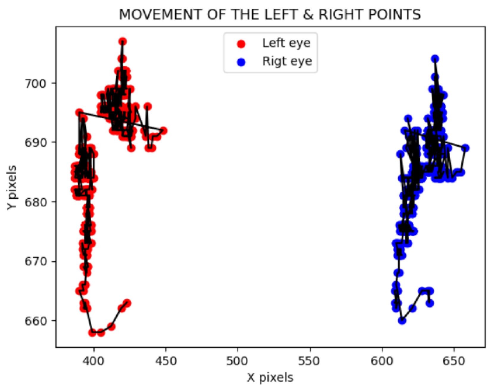
To extract this signal, the movement of each eye is calculated across each video frame, that is, the landmark of each eye in every frame along the X and Y axes -
Figure 2. Once these signals are obtained, one per eye, normalization is performed. The normalization of the signal, prior to the FFT, ensures that the amplitudes of the signals are comparable. A Min-Max normalization has been selected, which allows scaling the signal amplitude data between 0 and 1. The following formula has been applied for this purpose:
Let be the value of the normalized signal, the minimum amplitude value of the signal, and the maximum amplitude value of the signal.
Each movement in the X or Y axis results in two signals, one for each eye. To combine these signals into a single signal per axis, the average of the values from both eyes is calculated for the X axis and the Y axis for each frame. Once the movement signals are obtained, their impact on the plethysmographic signal is evaluated. This signal lies within a specific frequency range, between 0.67 and 4 Hz, corresponding to the human pulse interval. To determine if the previous movement signals interfere within this frequency range, they are converted to the frequency domain using a Fast Fourier Transform (FFT).
To eliminate the effect of movement, the final step will be to subtract this noise signal from the frequency spectrum of the plethysmographic signal of interest. This approach will help to attenuate the peaks generated by the noise and enhance those that contain relevant information for the final estimation.
However, the reduction of noise will depend on each specific signal, requiring more or less attenuation as needed. To determine the amount of reduction required, an Artificial Intelligence (AI) model has been developed to predict the attenuation factor based on the plethysmographic signal. Since the input of the model is the plethysmographic signal in the frequency spectrum, an architecture capable of relating a vector of values to infer patterns and features that help predict the required reduction factor was needed. The chosen architecture was a Convolutional Neural Network (CNN), as it meets all the established requirements.
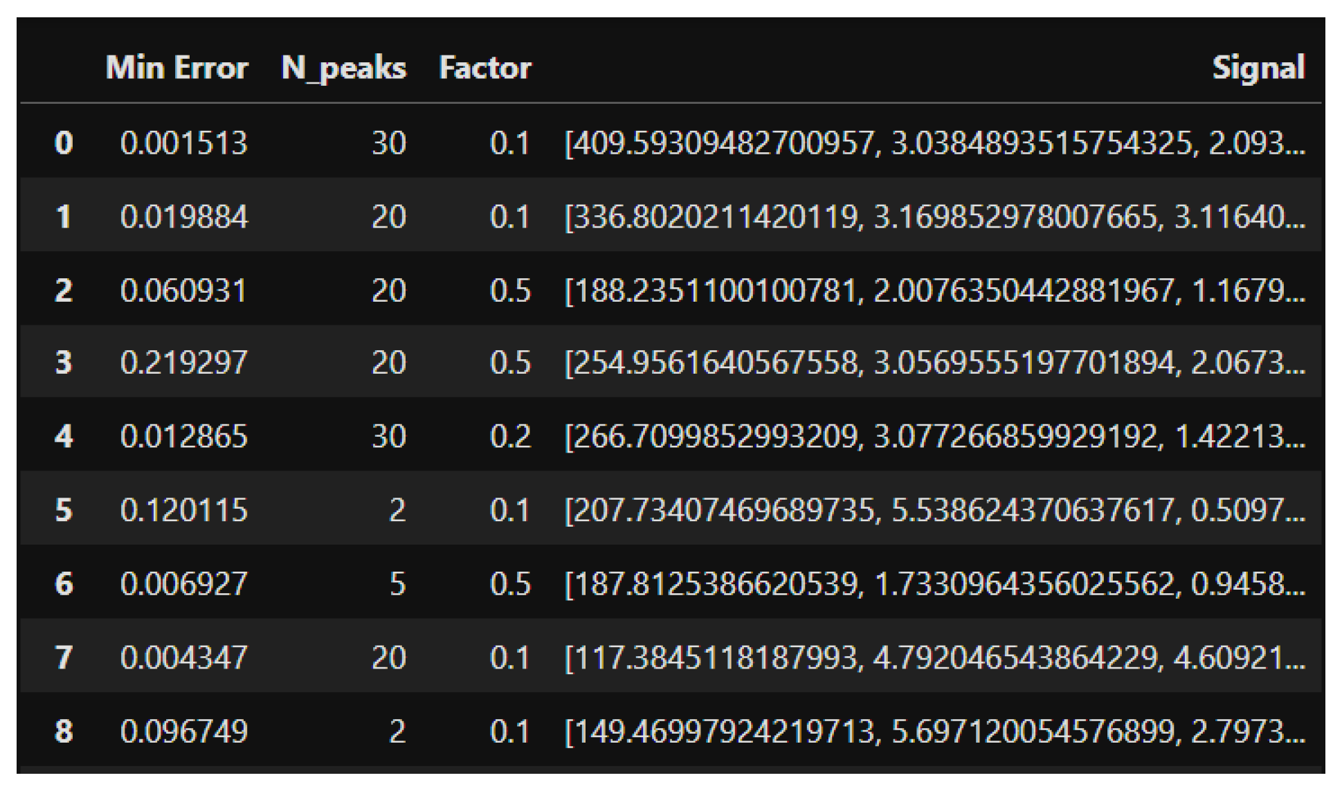
To extract the factor values used for the network’s learning, a Grid Search strategy was followed. This technique involves setting a range of parameter factor values and evaluating it based on the resulting errors of the method. The factor value with the lowest error for each of the input signals was set as the label or ground truth.
Figure 4 shows the input signal values, the target factor value used for training the model, and the error associated with that configuration.
The model training is performed using the Leave-One-Out Cross-Validation (LOOCV) technique [5]. This strategy maximizes data usage and avoids partition bias, as each data point is used in both the training and test sets. The network has the following hyperparameters:
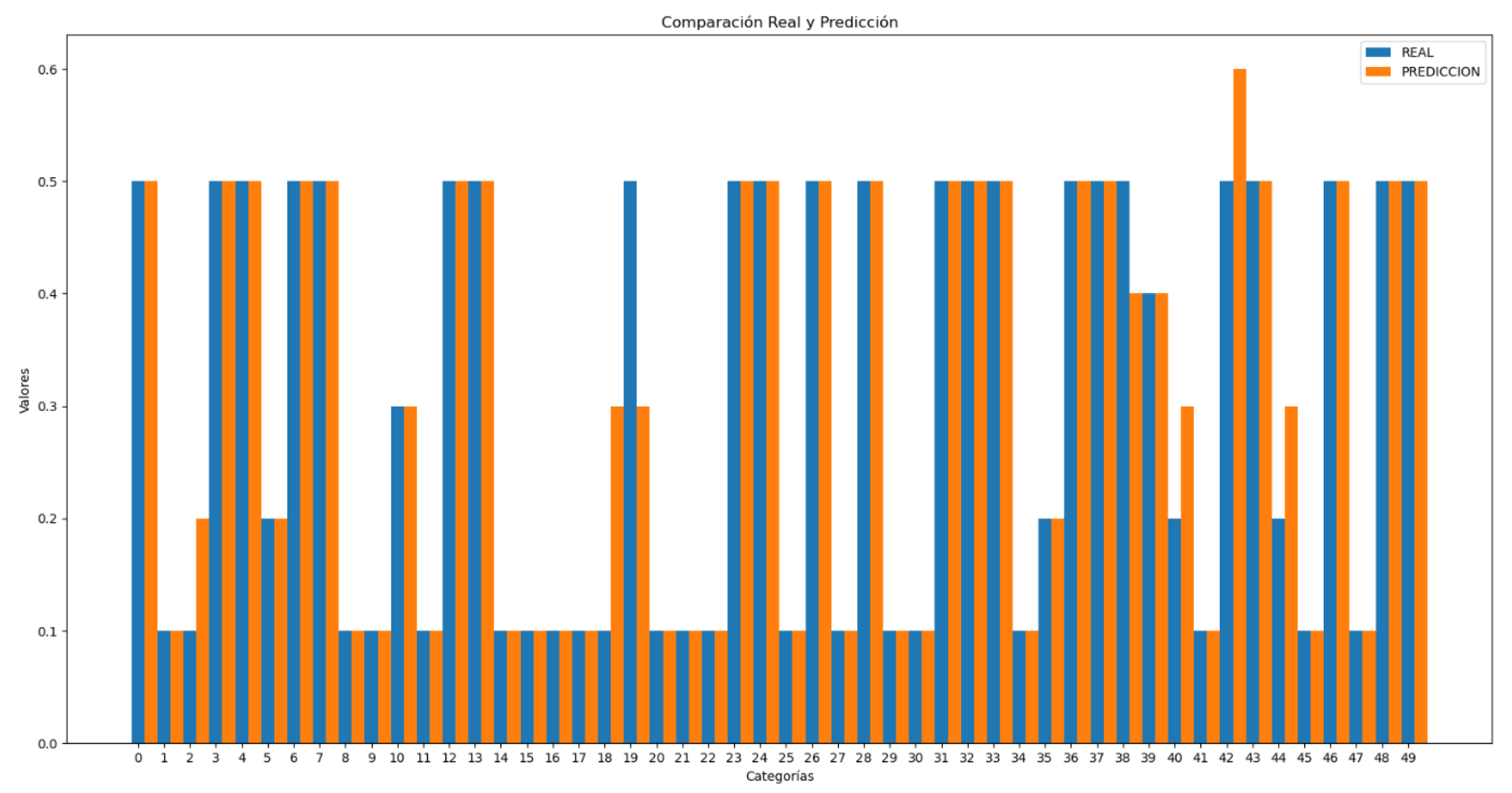
Figure 5 represents the comparison between the actual and predicted factor values by the CNN model for motion artifact removal:
3.1.3. Peaks Average
The preprocessing methods analyzed in the literature generally have the same goal: to process the signal so that, in the frequency spectrum, there is a peak with significantly higher amplitude than the others. This peak, when multiplied by 60, corresponds to the heart rate. The multiplication is necessary because the plethysmographic signal being used is filtered between 0.67 and 4 Hz, which corresponds to the normal human pulse frequency in beats per second. To convert it to the international unit, it needs to be transformed into beats per minute (bpm).
In summary, the frequency with the highest amplitude is chosen, converted to beats per minute (bpm), and selected as the heart rate. This choice is based on the assumption that this frequency represents the subject’s pulse, as it has a stationary component that pulses with considerable consistency. When analyzing the signal in the frequency domain, this consistency manifests as a prominent peak compared to other values [
12].
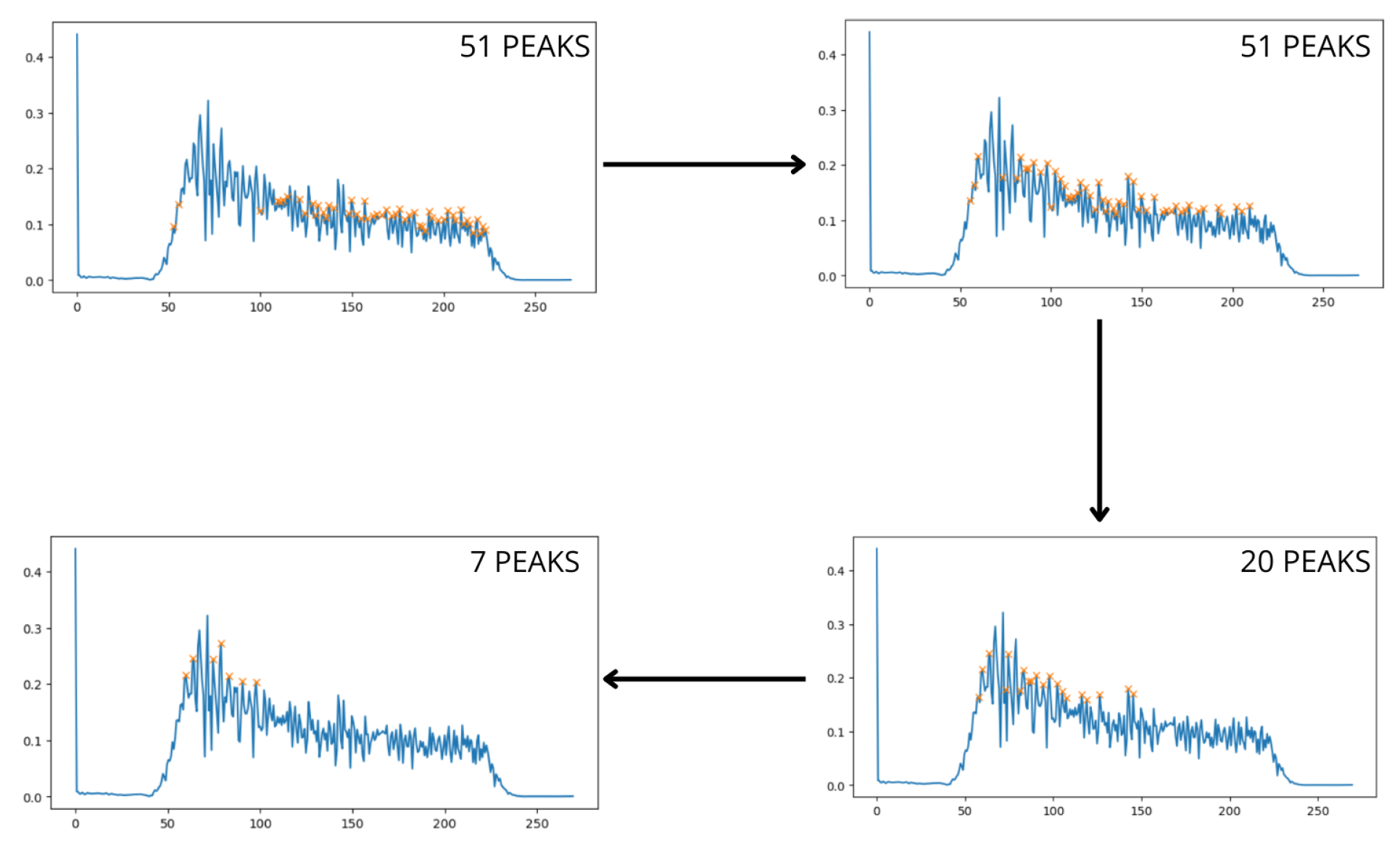
This ideal scenario is rarely encountered in practice, as various sources of noise, such as lighting, movement, and camera quality, can affect the signal. When noise is present, the signal no longer shows isolated and well-defined pulses, and other smaller peaks emerge around the main peak. In such cases, one can either average the frequencies of these peaks to approximate the true result or use the most prominent peak directly. The choice of method depends on the characteristics of the signal, but both approaches can keep the error within acceptable limits. However, the problem arises when, after filtering the signal within the range of interest, multiple high-amplitude peaks appear at disparate frequencies within this band, caused by noise. To address this challenge, an iterative process has been developed to progressively identify the peaks in the signal using a threshold that is iteratively adjusted. Initially, the threshold is set to zero and is progressively adjusted as peaks are detected within a defined range of peak mean ± standard deviation.
Figure 6.
Peak Detection Process
Figure 6.
Peak Detection Process
The process stops once a predetermined number of peaks have been detected [
11]. The higher this value, the more peaks will be considered for averaging, which will affect the final result. To optimize the stopping threshold value, an artificial intelligence (AI) model has been developed to predict the appropriate value, as the number of peaks to be considered will depend on the specific characteristics of the signal. The previous figure shows a real example in which the model has estimated that the most optimal value for peak selection is 7. This averaging allows the prediction to properly adjust to the actual value, resulting in a heart rate of 77.3 bpm, which is very close to the actual value of 79.4 bpm.
Similar to the previous motion noise reduction model, the input to the model consists of the discrete amplitude values of the plethysmographic signal in the frequency domain. Since the input data have different lengths, it is necessary to normalize them to a uniform size. For this task, a Convolutional Neural Network (CNN) is used, capable of identifying complex patterns and accurately estimating the result.
Like the AI model described in the previous section, this one also trains using the Grid Search technique.
Figure 4 shows the input data: on one hand, the plethysmographic signal in the range of interest within the frequency domain, and on the other, the target value,
associated with each signal. This
value represents the optimal number of peaks to consider to obtain the minimum error when estimating the heart rate, and it is therefore the value used as the label or ground truth when training the CNN.
Likewise, the training is carried out using the Leave-One-Out Cross-Validation (LOO-CV) strategy, due to the limitation in the amount of available data. The network has the following hyperparameters:
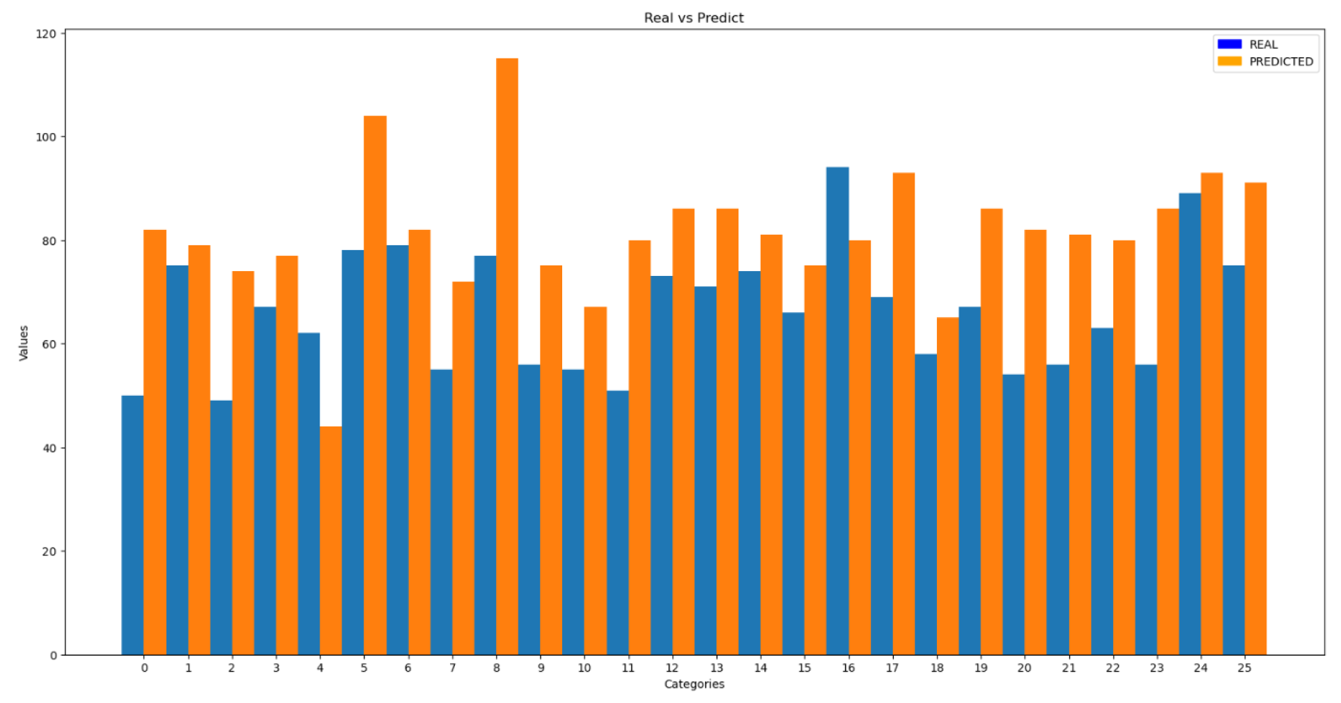
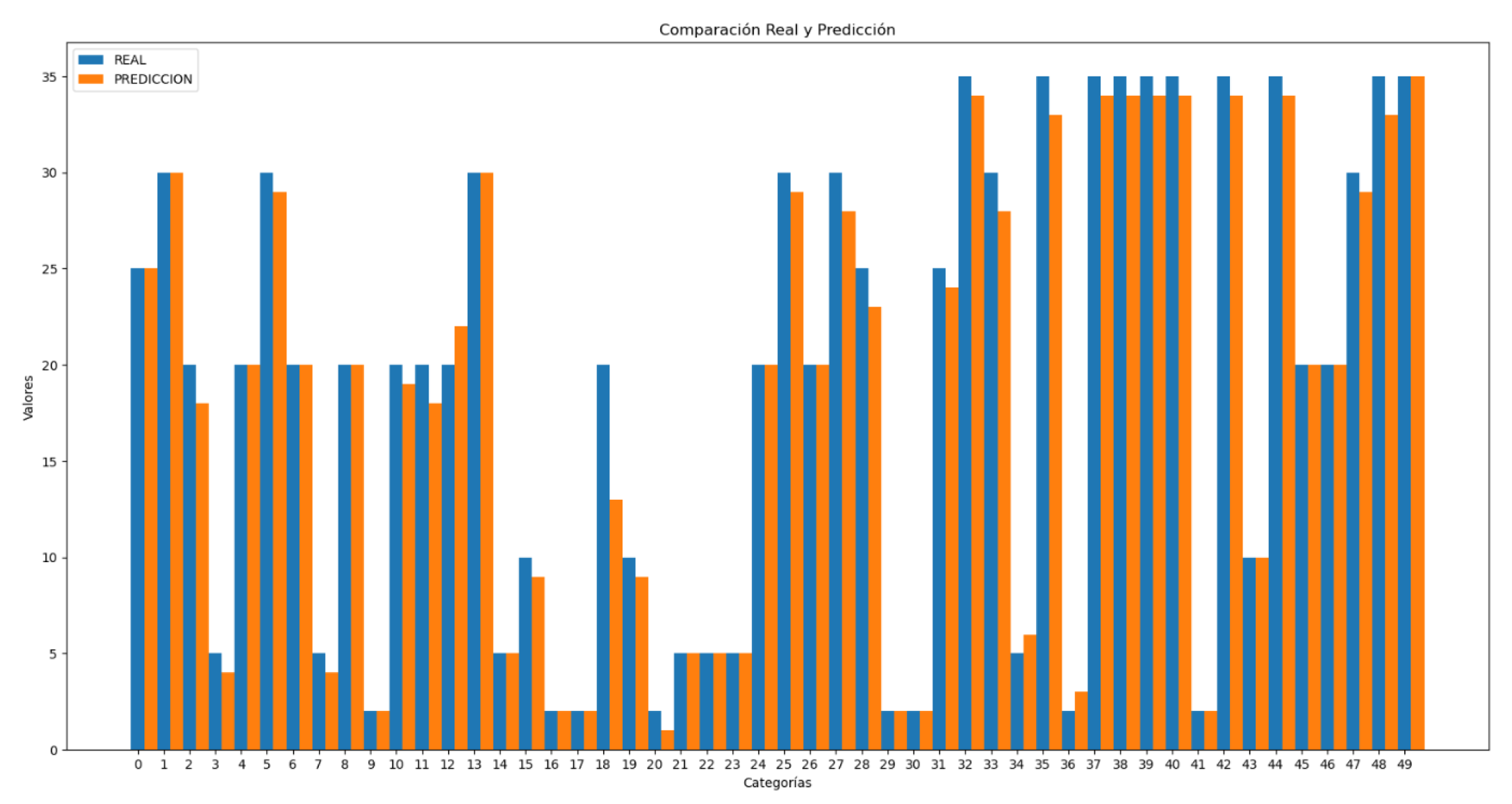
Subsequently, in
Figure 7, some comparisons between the actual values and those predicted by the model are presented.
3.2. Heart Rate
To summarize all the previous processes, the heart rate estimation is performed based on the resulting signal from the green channel of the video. This signal has had the noise caused by motion artifacts (
Section 3.1.2) attenuated, and a peak estimation adjustment (
Section 3.1.3) has been carried out, as these data will be input into the CNN estimation model.
3.2.1. Convolutional Neural Network
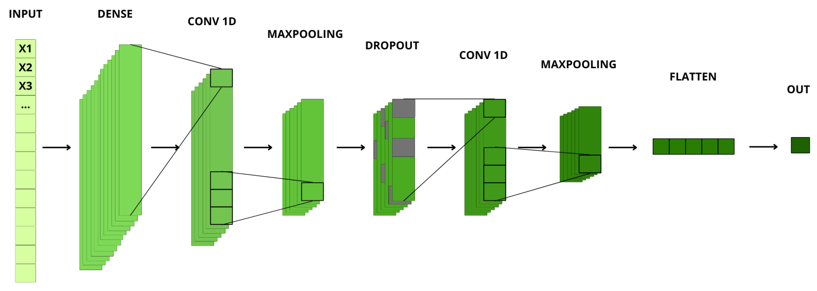
The chosen architecture for this purpose is a one-dimensional Convolutional Neural Network (CNN), as the input data for training is based on data vectors containing different information. Since the peak estimator model (
Section 3.1.3) generates a varying number of peaks depending on the signal, the vectors differ in length. To ensure a uniform length, zero padding is used. This padding helps avoid inconsistencies, ensuring that all input vectors have the same length, even if the number of relevant data points within them varies. After padding, all vectors have a length of 40 dimensions.
The CNN is particularly well-suited for this task due to its ability to identify and learn complex patterns and features in the input data. This capability is crucial because the variability in the plethysmographic signal requires an architecture that can adapt to different data structures while still producing accurate heart rate estimations. The CNN processes these vectors, correlating relevant features and filtering out noise to provide an accurate estimation of the final heart rate value.
Figure 9 shows all the layers that make up the AI model designed to estimate the final heart rate. This Convolutional Neural Network (CNN) is structured into multiple layers, each with specific parameters that contribute to feature extraction and estimation accuracy.
The model was trained using Leave One Out-Cross Validation (LOO-CV) [
13]. This approach allows for a more realistic evaluation metric, as the test set is never used during training. The model has the following hyperparameters:
In detail, the procedure is as follows. If there are a total of 72 videos, the dataset is divided into 72 parts. In each iteration, one video is used as the test set, and the remaining 71 videos are used as the training set. This process is repeated 72 times, changing the test set video in each iteration and recording the evaluation metric. After all iterations are completed, the average of the obtained metrics is calculated, providing an overall evaluation of the model. This strategy maximizes data usage, as every data point in the dataset is used for both training and testing, ensuring the maximum utilization of available information.
3.2.2. Multilayer Perceptron Regressor (MLPR)
After obtaining the initial heart rate estimation based on the CNN model defined in (3.2.1), a Multi-Layer Perceptron (MLP) is employed to refine the accuracy of the estimation. In this step, additional data from the subject, such as gender, age, and Body Mass Index (BMI), are introduced, as these factors can significantly influence heart rate. This final adjustment is made because there is correlation among these physiological parameters and heart rate. For example, heart rate can vary considerably based on an individual’s age, physical condition, and gender, as demonstrated in previous studies [
14].
The Multi-Layer Perceptron Regressor (MLPR) is used in this research to enhance the precision of heart rate estimation by taking into account the subject’s personal characteristics. This machine learning technique allows for continuous value predictions and is particularly useful in this context due to the variability of heart rate according to individual physiological conditions.
Since the research aims to optimize the application and user experience, the overall model needed to be lightweight to avoid long prediction times. For this reason, a pre-trained model from the "Scikit-Learn" [
15] library was utilized.
Scikit-Learn is a widely used machine learning library in Python for implementing and evaluating machine learning models. Within Scikit-Learn, the MLPRegressor is a class that implements a multi-layer perceptron for regression problems.
A multi-layer perceptron is a type of feedforward neural network that consists of one or more hidden layers between the input layer and the output layer. In this research, the Scikit-Learn MLPRegressor was used to fine-tune the heart rate estimation accuracy. This was achieved by incorporating personal data from the subject, such as gender, age, and Body Mass Index (BMI).
Figure 10 shows a summary of the methodology used for heart rate estimation. The peaks are recorded with the necessary information for the CNN model, the first estimation is performed, and finally, the final heart rate is estimated using MLPR
3.3. Blood Pressure
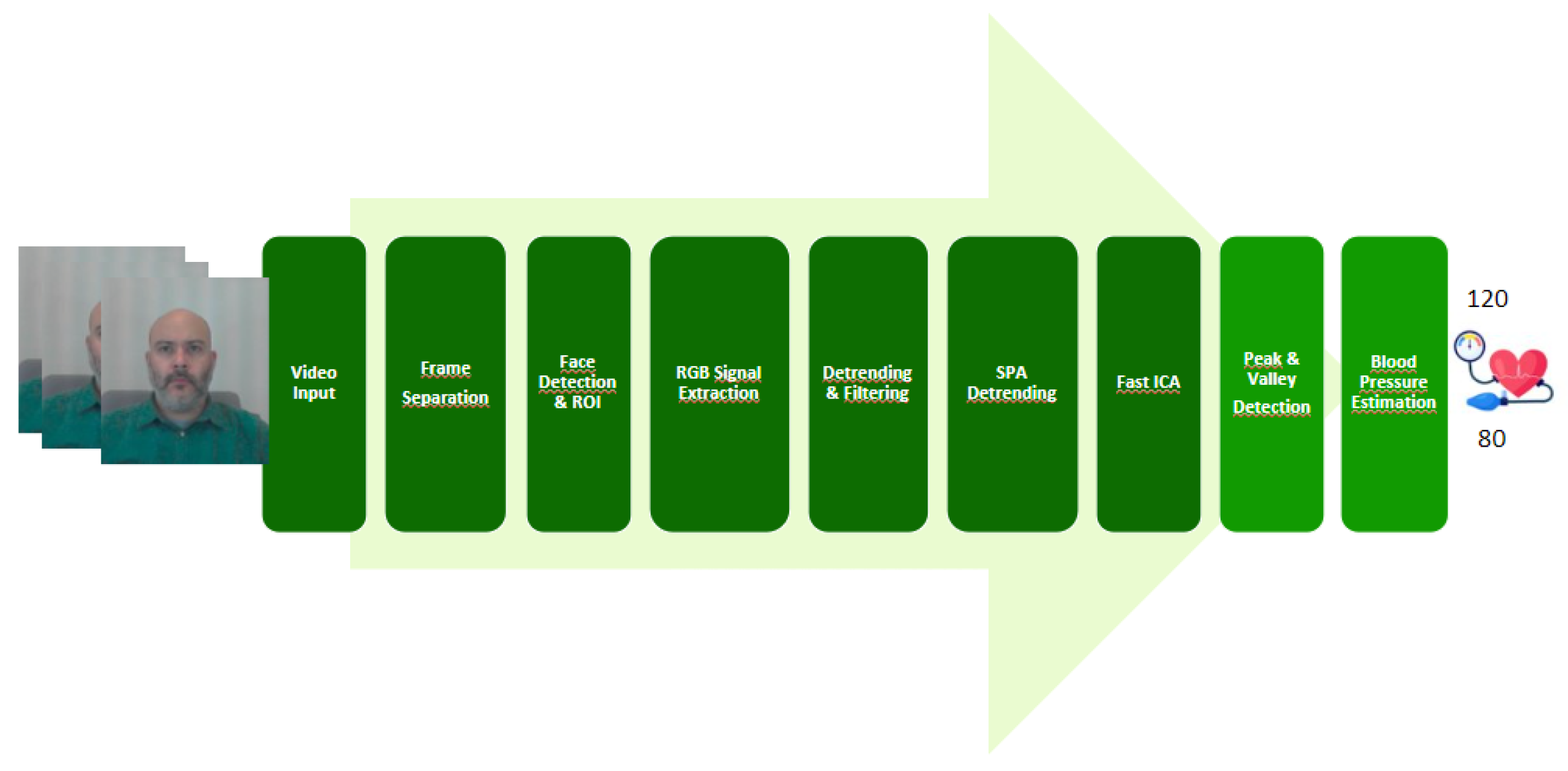
To reduce the effect of motion artifacts as well as other factors that can negatively impact the acquisition of the plethysmographic signal (rPPG), from which blood pressure estimation is derived, this section outlines the set of preprocessing techniques implemented in the AIVA project.
Figure 11 shows a series of processes discussed in section () Preprocessing, as it is common to both the heart rate estimation method and the blood pressure estimation method. However, once the RGB signals are obtained separately, the next step differs from the heart rate model; in this case, a ‘detrending and moving average filtering’ is performed.
3.3.1. Detrending & Moving Average Filtering
According to what is mentioned in [
12], the signals resulting from the decomposition of RGB channels are filtered using a 5-point moving average filter to smooth them, i.e., reduce noise and make the underlying trends more visible. After that, the stationary component is removed using the mean scaling and centering algorithm. The detrending and moving average filtering process is shown in the following equation [
16]:
Where m(t,l) = , with L representing the moving average of L points from the color vectors for channel i (in our case, ).
The primary objective of applying this equation is to eliminate the DC component of the signal in the resultant signals from the RGB channel decomposition, as well as to suppress high-frequency noise, thereby preparing the signal for subsequent analysis.
3.3.2. SPA Detrending
After performing the detrending of the signal as described in the previous section, a more flexible detrending process known as the Smoothness Prior Detrending Approach (SPA) is then applied. This technique, unlike the moving average method which uses a fixed set of points, offers improved accuracy by explicitly modeling the trend, even for complex and nonlinear trends. The procedure is as follows:
-
Definition of the Smoothness Prior:
a. In our case, the smoothness of the signal is penalized using the squared difference of the signal components, that is,
-
Definition of the Detrending Function
a. The detrending function combines the fidelity to the original signal with the smoothness of the trend, and is defined as follows:
i. The first term aims to remove the linear trend or slope of
by subtracting the original signal values
from the estimated values
, where
is the result of modeling
as a linear regression.
ii. The second term represents the square of the second derivative of the function and penalizes rapid variations in the signal.
iii. is the smoothing parameter that controls the balance between the fidelity to the signal and the smoothness of the fit, effectively preventing excessive smoothing of the function.
Figure 12.
SPA Detrending Process
Figure 12.
SPA Detrending Process
To determine the parameter that provided the best performance, a grid search was conducted. Specifically, for a range of values between 0.01 and 0.0001, the model’s performance was evaluated. The results demonstrated that offers the best trade-off between signal fidelity and smoothness of the fit.
Table 1.
Grid Search Results for the Performance Parameter
Table 1.
Grid Search Results for the Performance Parameter
|
value |
0.001 |
0.08 |
0.001 |
0.0015 |
0.0001 |
| Systolic Error |
0.029019 |
0.012015 |
0.059270 |
0.056503 |
0.039644 |
| Diastolic Error |
0.063691 |
0.077609 |
0.032232 |
0.033700 |
0.051969 |
3.3.3. Fast ICA
After removing the trend from the signal using the proposed methods, the next step is to apply Blind Source Separation (BSS) techniques. These techniques enable the extraction of original source signals from a set of mixed signals, where the sources are combined. In other words, from mixed signals that result from a set of source signals, the goal is to recover the original sources from these mixtures, with minimal or no information about the sources or the mixing process.
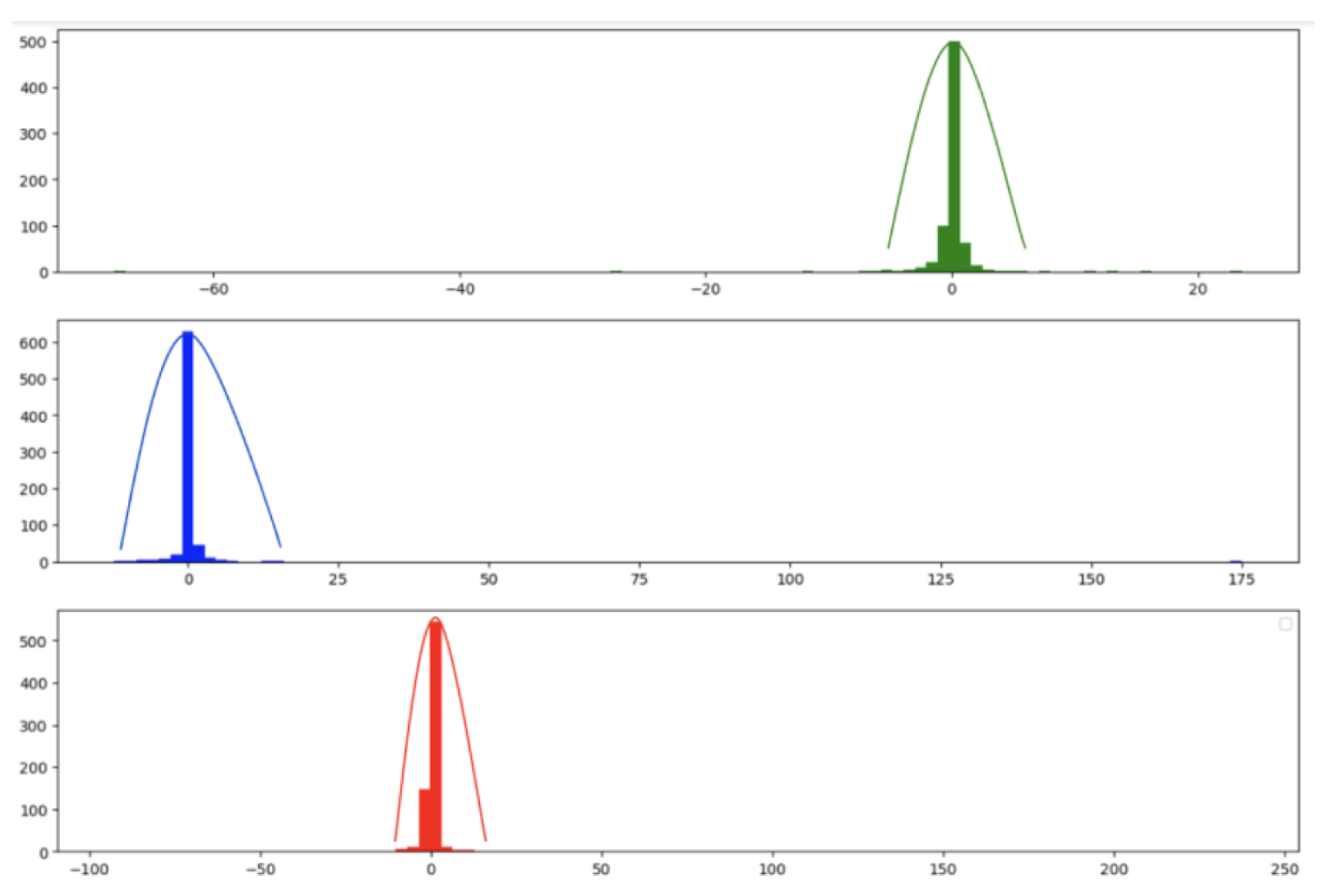
There are various methods for blind source separation. In this paper, we focused on Independent Component Analysis (ICA) as it provided good results and is the most frequently used method in the literature. ICA is a computational method used to separate a mixed signal into additive subcomponents that can potentially reconstruct the original signal. The method starts with the mixed signal, assuming it has a Gaussian-like behavior, and applies techniques to reduce the Gaussianity of this mixed signal, under the assumption that the subcomponents are non-Gaussian and statistically independent. The following figure shows the distribution functions of the amplitudes of the R, G, and B channel signals before applying FastICA, and it is observed that they exhibit some Gaussian behavior.
Figure 13.
Gaussianity of Signals Before Applying Fast ICA
Figure 13.
Gaussianity of Signals Before Applying Fast ICA
Several versions of ICA exist; however, we have focused on the Fast ICA algorithm [
17]. This algorithm is an optimized version that makes the ICA process faster and more efficient. In our case, Fast ICA is applied to the extracted signal RGB channels (3.1), resulting in 3 components. To determine which component represents the PPG signal and which are sources of noise, each of these components is transformed into the frequency domain using FFT and filtered within the range of interest using a Chebyshev Type II filter, as it is a low-pass filter characterized by an attenuation band with a ripple zone and a flat passband with a rapid transition. The component with the most prominent peak in the frequency band of interest is selected as the one containing the photoplethysmography information.
Figure 14.
Independent components
Figure 14.
Independent components
3.3.4. Peak and Valley Detection
After applying FastICA and selecting the component with the maximum peak within the frequency spectrum, this stage involves counting the peaks and valleys of the signal.
According to the Radial Resonance Theory [
18], the arterial system can be considered similar to a blood wave transmission system. This approximation allows for the development of a model capable of predicting blood pressure based on equations and properties of the arteries. Using the captured frames, the arterial pulse signal can be filtered, and the peaks and valleys, which are considered systolic and diastolic pressures, can be continuously estimated.
Along with the periodic cardiac contraction activities, the light incident on the face is absorbed and attenuated by the skin, muscles, and blood, so that the intensity of the reflected light detected by the optical receiver is weakened. During heart contraction, the volume of peripheral blood is greater, leading to significant light absorption, and the detected light intensity is at its minimum; whereas when the heart is in a diastolic state, in contrast, the detected light intensity is at its maximum.
Figure 15.
Blood Pressure signal
Figure 15.
Blood Pressure signal
Using the BMI measure [
19] as a correction coefficient and fitting an equation described in the Radial Resonance Theory, where the heart is described as a cyclic pressure pump, the following equation is obtained:
Where
is the function to be fitted;
is the BMI correction coefficient; and
x is the average of all peaks or valleys in the signal. The averages of peaks and valleys are extracted using the following equations:
Where
and
represent the number of peaks and valleys, respectively;
and
are the amplitude values of the peaks and valleys. When counting the number of peaks and valleys, those whose separation is less than the following equation have been omitted:
Where represents the beats per second of the subject, derived from the heart rate, and represents the frames per second at which the video is captured.
According to the experiments defined in [
20], the parameters
of the function
have been determined using a least squares fit of the blood pressure measurements present in our dataset, resulting in the following equations for systolic blood pressure (SBP) and diastolic blood pressure (DBP):
4. Results and Discuss
To obtain the final results, two evaluation metrics were used. First, the CNN model used to estimate the heart rate was trained with the mean squared error (MSE) loss function, which is the mathematical function that evaluates the discrepancy between the model’s predictions and the actual values. It is a quantitative measure that indicates how well the model is performing its task. Its equation is as follows:
Additionally, for the final evaluation of heart rate (at the output of the MLPR) and for the blood pressure prediction, the Absolute Relative Error (ARE) was used as the evaluation metric. This metric measures the relative error between predicted and actual values, providing a measure of the model’s accuracy in relative terms.
This approach has enabled a comprehensive and accurate evaluation of the model, ensuring that the estimated performance accurately reflects its generalization ability. By using ARE, it has been possible to clearly and precisely quantify how much the model’s predictions differ from the actual values, thereby providing a robust metric for the final evaluation of the model.
In order to demonstrate the capability of the models for blood pressure and heart rate estimation, we compared the results from our models to a blood pressure monitor. This comparison was carried out with 10 participants aged between 25 and 40 years. Each participant underwent between two and three tests conducted over several days and at different times, thus maximizing the variability and representativeness of the measurement conditions. To compare the estimation, the actual measurements of heart rate and blood pressure were collected simultaneously with the video using a sphygmomanometer.
The following figure shows the results of the predictions compared to the actual data.
Figure 16.
Comparison of Results for Heart Rate
Figure 16.
Comparison of Results for Heart Rate
To quantitatively verify the results, the Average Relative Error (ARE) was used, yielding an error of 28%, which is considerably higher than the error obtained with the test set in previous trials. In addition to the ARE, the standard deviation of the results was calculated, resulting in a value of 12.9.
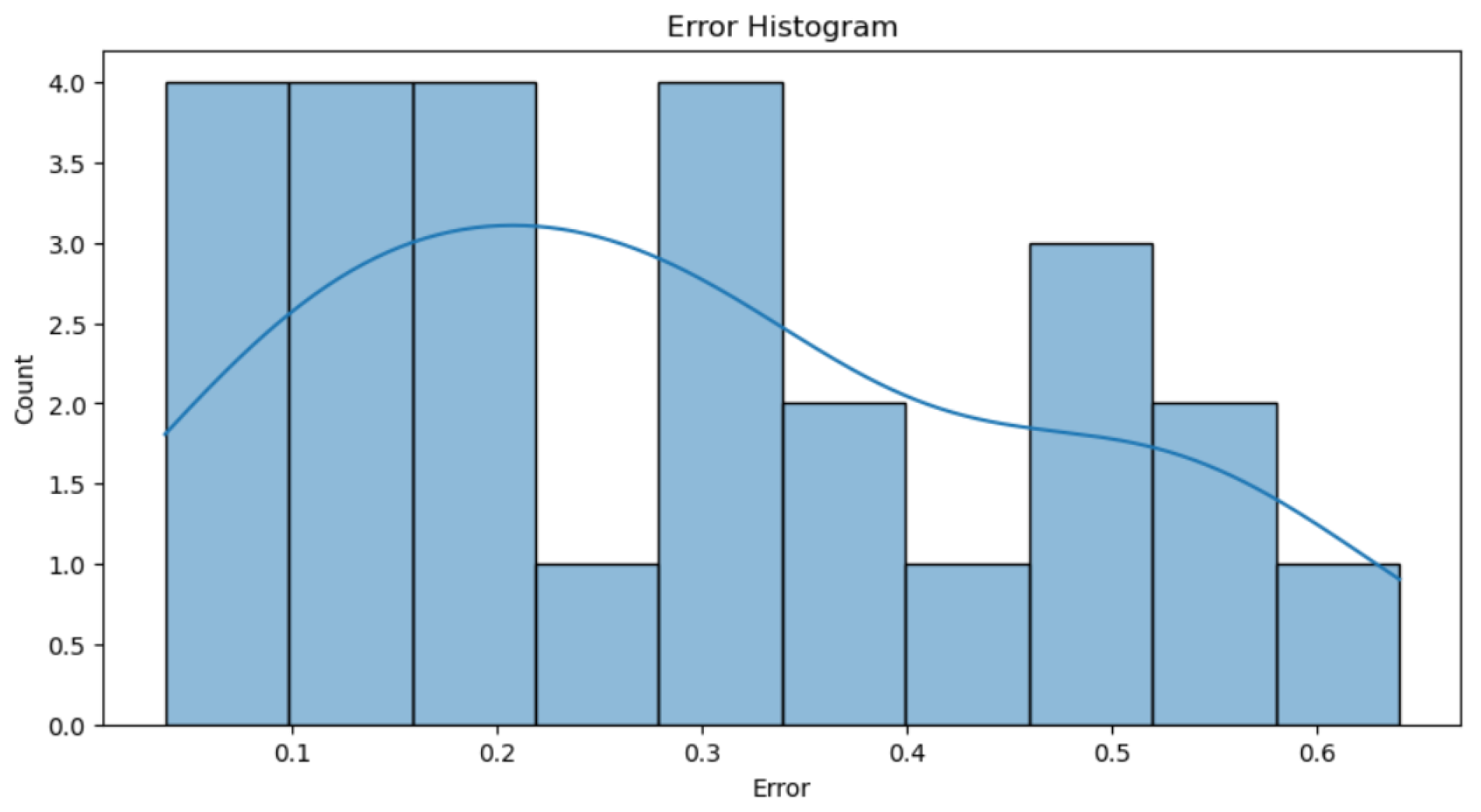
Analyzing the errors shown in
Figure 17, it is observed that the percentage of error obtained is largely due to those values with an error greater than 0.4, as these significantly penalize the total error. Beyond this threshold, there are few cases with considerably higher errors compared to the rest, but these cases have a notable impact on the total error computation. The trend line indicates that there are more errors near an error of 0. Additionally, it suggests that while most predictions are reasonably accurate, large and isolated errors disproportionately increase the average error metric, highlighting the need to improve the model to better handle these outliers.
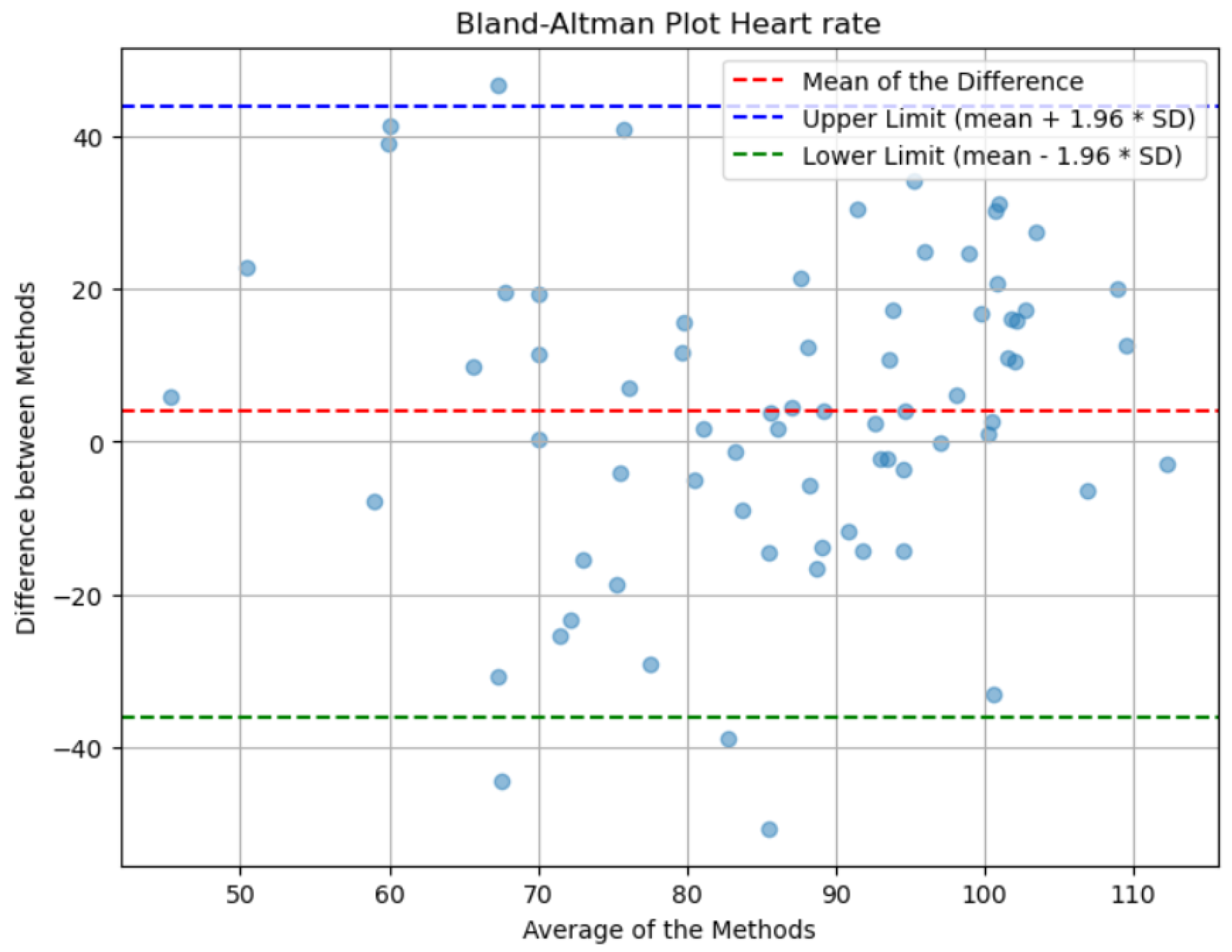
Lastly, the analysis of the Bland-Altman plot presented in
Figure 16 shows that the mean of the differences between the actual and predicted values is close to zero, indicating that, on average, there is no significant discrepancy between the actual measurements and the model’s estimates. This suggests that the predictions do not exhibit a systematic bias towards higher or lower values. Additionally, the dispersion of the points across the range of measurements reflects consistent variability, which is indicative of a uniform distribution of errors throughout the spectrum of evaluated values. It is worth noting that the lines of agreement, which show the range within which most differences fall, are too wide due to the method’s error.
Blood pressure prediction has been divided into systolic (high) and diastolic (low) pressures, with values estimated separately.
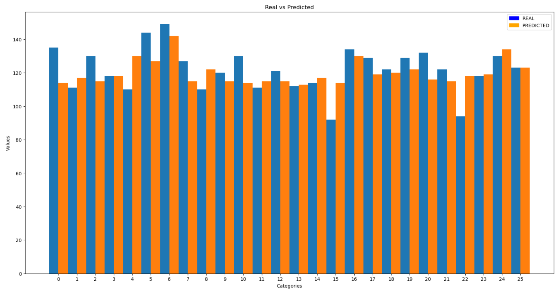
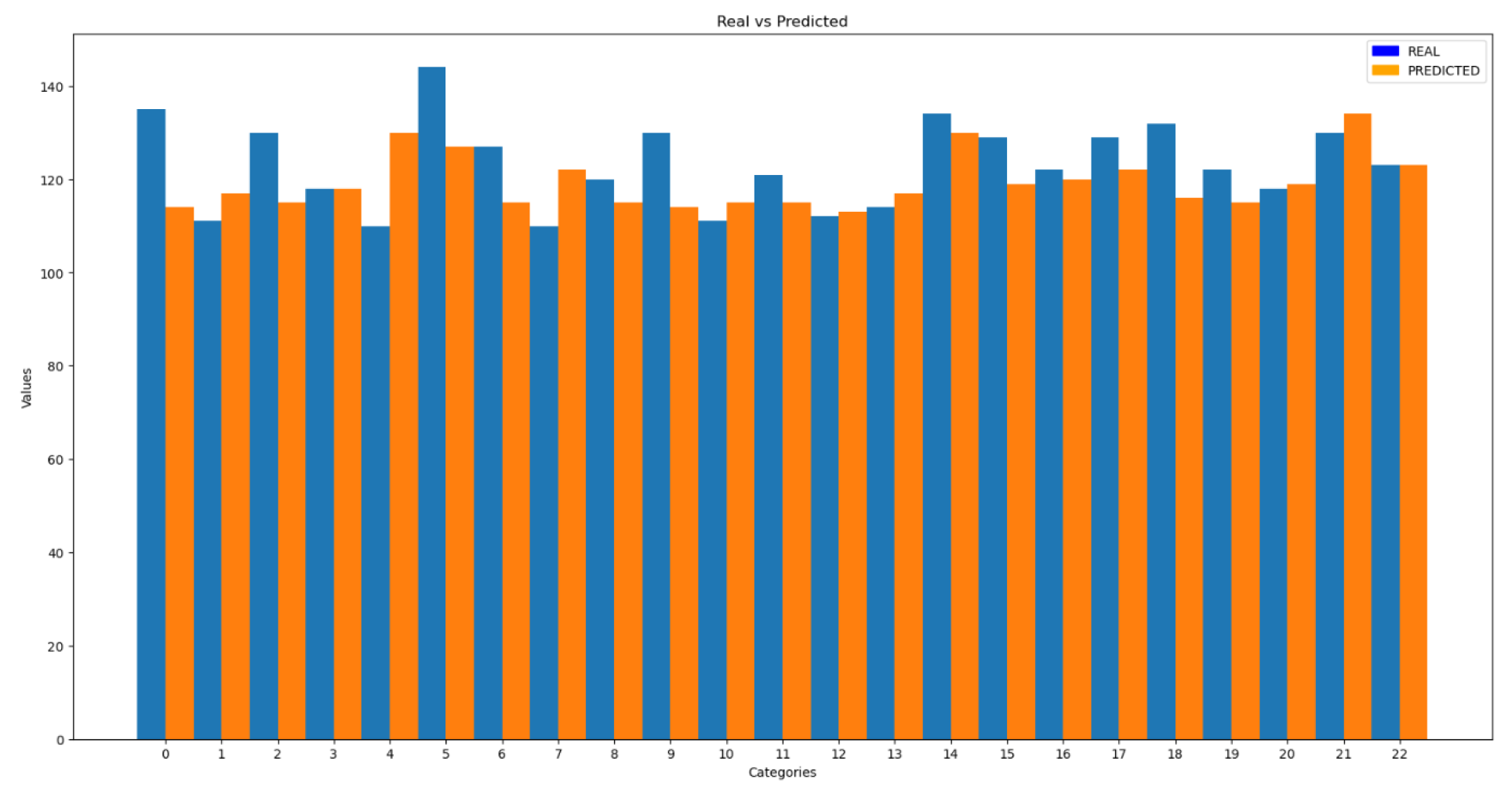
The comparisons between real and predicted values shown in
Figure 19 and 20 are much more accurate than the heart rate comparison shown in
Figure 16.The results obtained for systolic blood pressure show an error of 7.8%, while for diastolic blood pressure the error is 9.5%. These values are comparable to the errors observed in the test set, indicating consistency in the model’s performance. Additionally, the standard deviation of the predictions was calculated, with values of 11.65 for systolic pressure and 9.62 for diastolic pressure.
In these graphs (
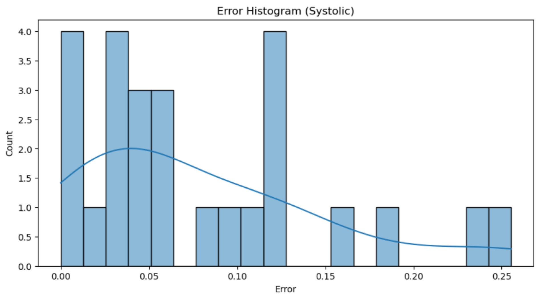
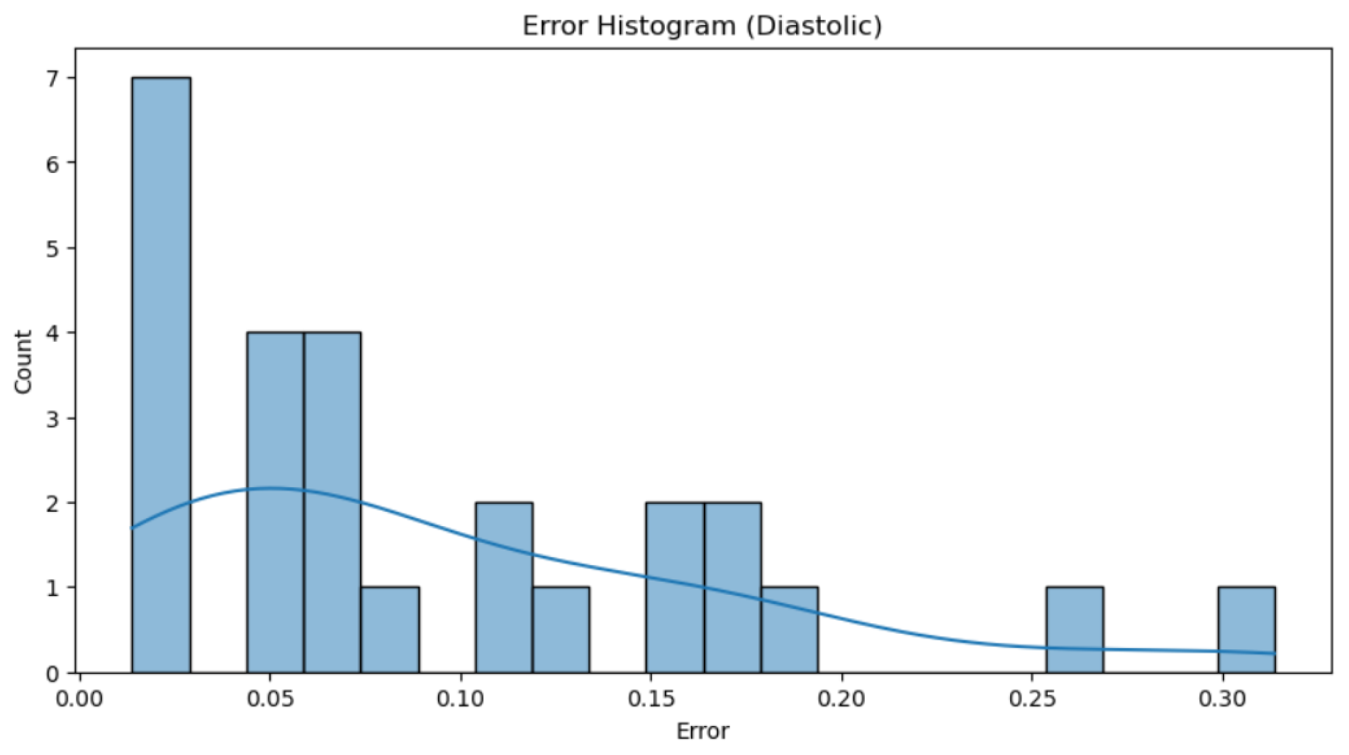
Figure 21 and 22), it can be observed that the majority of individual errors, both in systolic and diastolic pressure, are very close to zero. Although there are some errors that are more distant and disproportionately impact the total error, these are very few, especially in the case of diastolic pressure. This observation is clearly supported by the trend line representation, which visually shows the concentration of most errors near the zero value. From values of 0.15 in the first graph and 0.2 in the second, isolated errors appear, which can be attributed to exceptional cases such as reading errors.
Figure 21.
Histogram of Systolic Blood Pressure Errors
Figure 21.
Histogram of Systolic Blood Pressure Errors
Figure 22.
Histogram of Diastolic Blood Pressure Errors
Figure 22.
Histogram of Diastolic Blood Pressure Errors
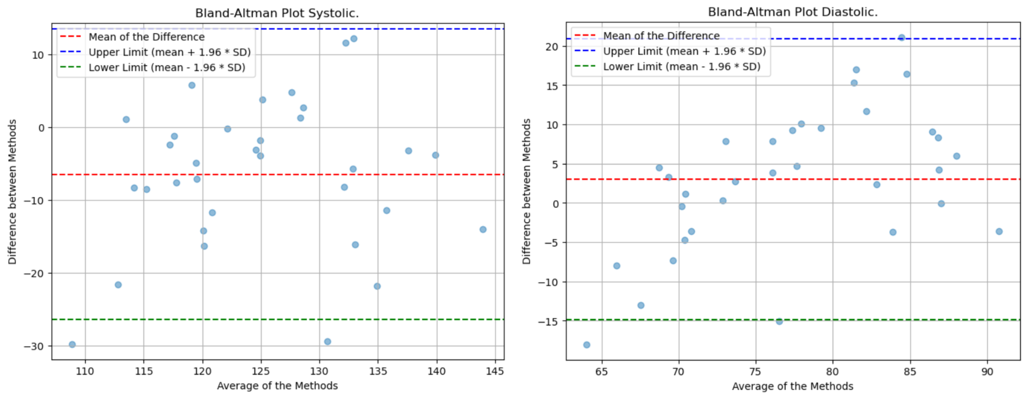
Figure 23.
Bland-Altman Blood Pressure
Figure 23.
Bland-Altman Blood Pressure
It is important to note that the average of the predicted values is very similar to the average of the actual values, indicating the absence of a systematic trend in the predictions towards higher or lower values. Additionally, the limits of agreement for systolic and diastolic pressure are significantly narrower compared to those for heart rate. This suggests that the deviation of values from the average is relatively small.
Table 2 summarizes the conclusion of errors and standard deviation for heart rate and blood pressure.
5. Conclusions
In this paper, a detailed evaluation was conducted of the artificial intelligence models designed for estimating heart rate and blood pressure through remote photoplethysmography (rPPG). The results provide a comprehensive view of the performance of these models under practical conditions.
The comparison among the estimated values and those from a blood pressure monitor demonstrated that the models can offer reasonably accurate estimates under a variety of conditions. However, significant limitations were also identified, particularly in predicting extreme values of heart rate and blood pressure. This phenomenon is largely attributed to the scarcity and imbalance of training data in those specific ranges.
The result of the heart rate evaluation, using the ARE metric, was 28%, notably higher than the 13% obtained in the test set, highlighting the need for a more balanced and representative dataset. On the other hand, systolic and diastolic blood pressure predictions showed errors of 7.8% and 9.5%, respectively, values similar to those obtained during the test phase, indicating good consistency in these predictions.
When comparing these results with those obtained in other references, it is noteworthy that our heart rate model shows greater deviation compared to traditional methods such as ICA or PCA. These methods were evaluated in the project and did not provide better results in our study, mainly due to the limitations of our dataset.
References
- Poh, M. Z. , McDuff, D. J., & Picard, R. W. Non-contact, automated cardiac pulse measurements using video imaging and blind source separation. Optics express, 2010, 18, 10762–10774. [Google Scholar]
- Kado, S. , Monno, Y., Moriwaki, K., Yoshizaki, K., Tanaka, M., & Okutomi, M. Remote heart rate measurement from RGB-NIR video based on spatial and spectral face patch selection. In 2018 40th annual international conference of the IEEE engineering in medicine and biology society (EMBC), 2018, 5676–5680.
- Yang, F.; He, S.; Sadanand, S.; Yusuf, A.; Bolic, M. Contactless measurement of vital signs using thermal and RGB cameras: A study of COVID 19-related health monitoring. Sensors 2022, 22, 627. [Google Scholar] [CrossRef] [PubMed]
- Secerbegovic, A. , Bergsland, J., Halvorsen, P. S., Suljanovic, N., Mujcic, A., & Balasingham, I. Blood pressure estimation using video plethysmography. In 2016 IEEE 13th international symposium on biomedical imaging (ISBI), 2016, 461–464.
- Iwashita, Y. , Nagumo, K. , Oiwa, K., & Nozawa, A. Estimation of resting blood pressure using facial thermal images by separating acute stress variations. Artificial Life and Robotics, 2021, 26, 473–480. [Google Scholar]
- Luo, H. Yang, D., Barszczyk, A., Vempala, N., Wei, J., Wu, S. J., ... & Feng, Z. P. Smartphone-based blood pressure measurement using transdermal optical imaging technology. Circulation: Cardiovascular Imaging,2019, 212(8).
- Wu, J. , Liang, H., Ding, C., Huang, X., Huang, J., & Peng, Q. Improving the accuracy in classification of blood pressure from photoplethysmography using continuous wavelet transform and deep learning. International journal of hypertension, 2021,2021.
- Google (2010). Mediapipe [Computer Software]. Google. Available online: https://ai.google.dev /edge/mediapipe/solutions/guide?hl=es-419.
- Bousefsaf, F. , Maaoui, C., & Pruski, A. Continuous wavelet filtering on webcam photoplethysmographic signals to remotely assess the instantaneous heart rate. Biomedical Signal Processing and Control, 2013, 8(6), 568–574.
- S. Bobbia, R. S. Bobbia, R. Macwan, Y. Benezeth, A. Mansouri, J. Dubois. Unsupervised skin tissue segmentation for remote photoplethysmography. Pattern Recognition Letters, 2017.
- Wu, B. F. , Huang, P. W., Lin, C. H., Chung, M. L., Tsou, T. Y., & Wu, Y. L. Motion resistant image-photoplethysmography based on spectral peak tracking algorithm, 2018, 6, 21621–21634. [Google Scholar]
- A. Bhattacharjee and M. S. U. Yusuf. A Facial Video based Framework to Estimate Physiological Parameters using Remote Photoplethysmography, 2021, 1–7.
- S. Hara et al. Optimización de parámetros del sensor de frecuencia cardíaca basado en PPG con cancelación de artefactos de movimiento mediante validación cruzada, 2017, 6, 73–76.
- Sánchez, G. L. Sánchez, L. L., & Suárez, A. D. Composición corporal y variabilidad de la frecuencia cardiaca: relaciones con edad, sexo, obesidad y actividad física. SPORT TK-Revista EuroAmericana de Ciencias del Deporte, 2015, 4(2), 33–40.
- Pedregosa, F. , Varoquaux, Ga"el, Gramfort, A., Michel, V., Thirion, B., Grisel, O., … others. (2011). Scikit-learn: Machine learning in Python. Journal of Machine Learning Research, 12(Oct), 2825–2830.
- Gerard de Haanand Vincent Jeanne. "Robust Pulse Rate from Chrominance-Based rPPG”, IEEE Transactions on Biomedical Engineering, 2013, 2873–2886.
- A. Hyvärinen and E. Oja. A Fast Fixed-Point Algorithm for Independent Component Analysis. Neural Computation, 1997, 9(7), 1483-1492.
- Wang, Y. Y. L. , Jan, M. Y., Wang, G. C., Bau, J. G., & Wang, W. K. Pressure pulse velocity is related to the longitudinal elastic properties of the artery. Physiological Measurement, 2004, 25(6), 1397.
- M. Higuchi, K. Sorachi, and Y. Hata. Health checkup data analysis focusing on body mass index, 2017, 8, 1634–1641.
- Yimin Zhou, Member, IEEE, Haiyang Niy, Qi Zhang and Qingtian Wu, Member, IEEE. The Noninvasive Blood Pressure Measurement based on Facial Images Processing, 2015, 14, 1–11.
|
Disclaimer/Publisher’s Note: The statements, opinions and data contained in all publications are solely those of the individual author(s) and contributor(s) and not of MDPI and/or the editor(s). MDPI and/or the editor(s) disclaim responsibility for any injury to people or property resulting from any ideas, methods, instructions or products referred to in the content. |
© 2024 by the authors. Licensee MDPI, Basel, Switzerland. This article is an open access article distributed under the terms and conditions of the Creative Commons Attribution (CC BY) license (http://creativecommons.org/licenses/by/4.0/).
