1. Introduction
Tribology is fundamental to the development and improvement of materials used in mechanical, automotive, aerospace, and energy industries. Within this field, the tribological performance of composite materials is of particular interest due to their diverse applications and the ability to tailor their properties for specific uses. The tribological performance of these materials is primarily evaluated using two key parameters: the friction coefficient and specific wear rate, which describes the volume loss of the base material relative to the sliding distance and normal force. These indices provide crucial insights into the efficiency and durability of materials under various working conditions. Determining these coefficients typically involves analyzing data from tribological experiments over various periods. Nowadays, tribological tests at the model test level, such as pin-on-disk or block-on-ring tests, are usually carried out at a constant pv level over a period of around 24 hours. The tribological characteristic values such as coefficient of friction and wear rate are calculated integrally from all the data measured during this period. However, it's often overlooked that the system undergoes a running-in phase before transitioning to a stationary phase, where the coefficient of friction and wear rate remain constant. The duration of this running-in phase can significantly affect the traditionally calculated characteristic values. Therefore, it's advisable to distinguish between the running-in phase and the stationary phase when determining the tribological characteristic values.
Many researchers now manually identify the so-called “stationary phase” from the data or using analytical mathematical methods. However, the manual process is very time-consuming and subject to human error, as the time required to reach stable states varies with different materials and experimental conditions and the mathematical methods are often subject to errors, so a manual follow-up check is necessary. Recent advances in computational power and machine learning technologies have significantly enhanced the capabilities of artificial neural networks (ANNs), expanding their application across various scientific and engineering disciplines, including tribology. In 1997, Jones et al. [
1] attempted to use commercial artificial neural networks to predict the outcomes of pin-on-disc experiments involving composite materials and steel. Their models, utilizing various network architectures, achieved a prediction accuracy with R
2 values of approximately 0.9 for the Pin-on-Disc experiments. Subsequent ANN tribology studies [
2,
3,
4,
5,
6,
7,
8,
9] have built upon this pioneering work, as well as our own research [
10,
11,
12,
13], by refining ANN architectures and selecting appropriate algorithms. These efforts have demonstrated the feasibility of using ANN technology for predicting the tribological performance of both pure and reinforced polymers. In recent decades, the development of neural network technology has led to significant improvements in predicting the tribological performance of tribomaterials, particularly regarding the friction coefficient and wear rate. In 2011, Gyurova et al. [
6] employed the Variable Learning Rate Backpropagation Algorithm (GDX) to predict the friction coefficient (CoF) of polyphenylene sulfide (PPS), achieving an accuracy with a Mean Relative Error (MRE) of approximately 0.1. Subsequently, in 2013, Busse et al. [
14] enhanced this predictive accuracy by about 40% using the Levenberg-Marquardt Algorithm (LM), resulting in an MRE of approximately 0.059 for the same material and experimental data. In our previous study [
15], a series of PEEK-based composites with varying filler proportions were optimized for their tribological performance. And the material formulations were also included as input features during the construction and training of the neural network. Ultimately, the tribological performance of materials that had not undergone any actual tribological experiments was predicted based solely on their formulations and loading conditions. A comparison between the predicted results and the experimental data showed that the well-trained neural network achieved a high prediction accuracy, with an CoF-MRE of 0.062.
The aforementioned studies have primarily focused on the simulation and prediction of the tribological performance of materials, which is indeed one of the most critical objectives and outcomes in the field of tribology. These applications of neural networks are based on experimental data, utilizing different backpropagation optimization algorithms to construct and train the network models. Essentially, these are regression problems aimed at solving the task of mapping various inputs to their corresponding outputs. However, the functionality of neural networks extends far beyond regression tasks. Various types of neural networks are highly effective in handling tasks such as clustering, image recognition, and natural language processing. Despite the broad capabilities of neural networks, research in tribology has rarely explored applications beyond predicting tribological performance [
16,
17,
18,
19]. For instance, Aiordachioaie D. et al. [
20] utilized adaptive linear neural networks (ADALINE) and recurrent neural networks (RNN) to process and learn from acoustic signals of rolling mills, providing an effective tool for fault detection and structural changes in industrial processes through spectrum compression and classification. Yin F. et al. [
21,
22] employed a convolutional neural network-long short-term memory (CNN-LSTM) model to learn the friction coefficient variation over time for different friction pairs under seawater lubrication conditions, achieving predictive capabilities that save experimental time and costs. Motamedi N, in his study [
23], used convolutional neural networks (CNN) for stability classification of contact surfaces in tribological systems, recurrent neural networks (RNN) to analyze and predict contact surface temperature variations, and generative adversarial networks (GAN) to simulate and predict the evolution of contact surface roughness. These applications demonstrate the potential of neural networks in optimizing system performance and reducing experimental costs and time.
In the present study, artificial neural networks (ANNs) are innovatively applied for the batch analysis and processing of experimental data. Utilizing the capabilities of long short-term memory (LSTM) networks, which specialize in handling time series data, the network is trained based on experimental data from polymer-based composites and steel friction pairs. This enables the efficient and accurate identification of the so-called stationary phases in the experimental data, from which relevant tribological characteristics, such as friction coefficients (CoF) and specific wear rate (ws), can be extracted. Unlike neural networks designed to predict the tribological performance of tribomaterials under various working conditions, this study extends beyond focusing on specific materials and aims to establish a general tool for processing experimental data within the field of tribology. It is anticipated that this research will significantly enhance the efficiency of experiments and subsequent data processing, achieving automation from experimental execution to the production of analytical results.
2. Methodology
2.1. Task Definition and Network Choose
Two key parameters are typically used when characterizing
the performance of tribomaterials: the coefficient of friction (CoF) and the
specific wear rate (w
s). These parameters are derived from the data
recorded during tribological tests. In this study, a large amount of
tribological test data was utilized, originating from previous experiments on
polymer-based tribomaterials paired with steel counterparts. The CoF and w
s
are calculated from the time-dependent curves of the CoF and sample height
loss.
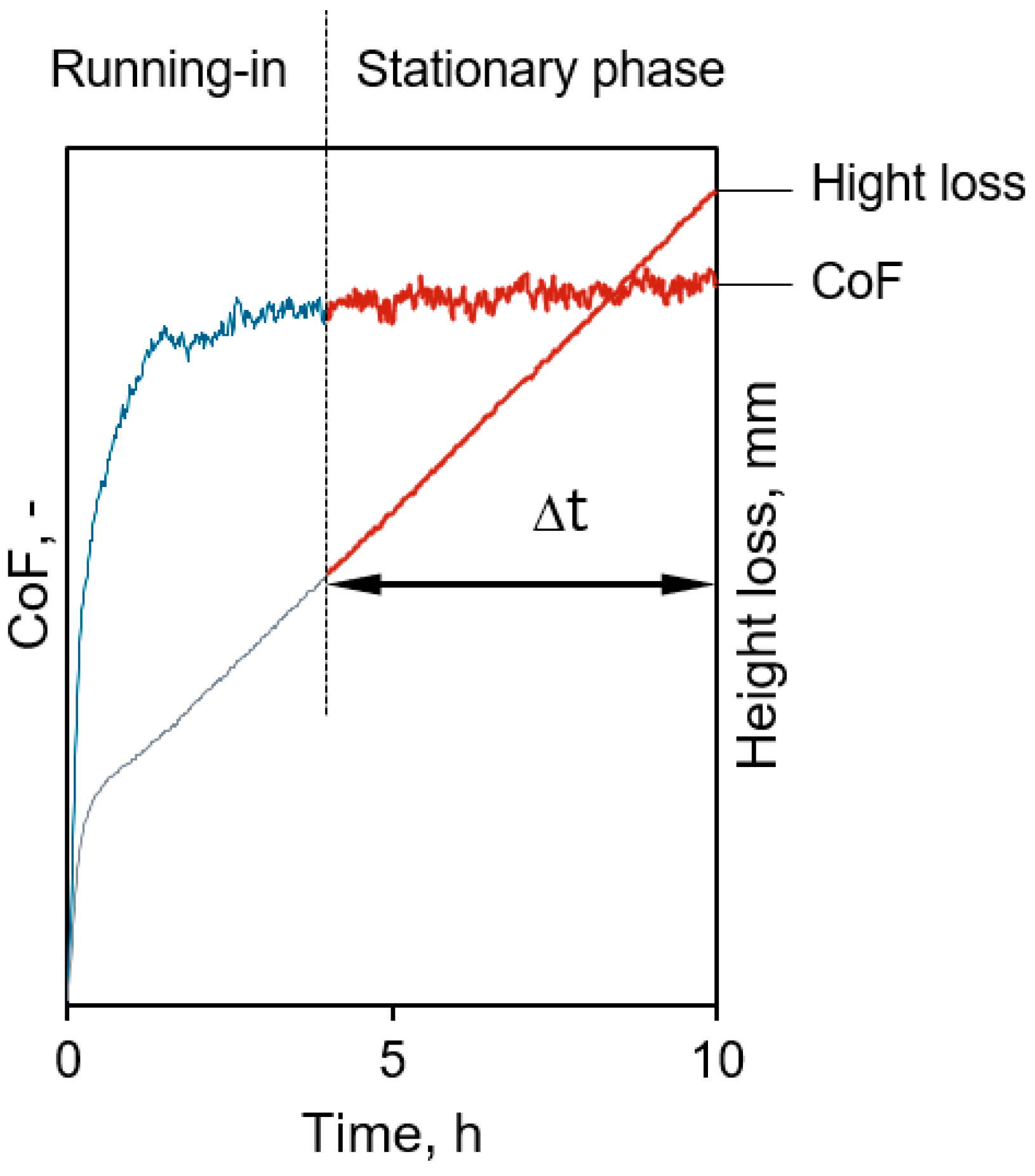
Figure 1 illustrates a typical
tribological test curve, showing that after an initial period, the CoF curve
and the slope of the height loss curve stabilizes within a narrow range,
continuing until the end of the experiment. This part of the curve is defined
as the stationary phase of this test whereas the part before reaching this
phase is termed the running-in phase, as described in DIN ISO 7148-2:2014-07 [
24]. The final CoF for this test is determined as
the average CoF during the stationary phase, the height loss during this phase
is used to calculate the wear rate according to the following equation:
where ∆h is the sample height loss in the stationary phase, p denotes the surface pressure, v is the sliding speed, and ∆t connotes the duration of the stationary phase.
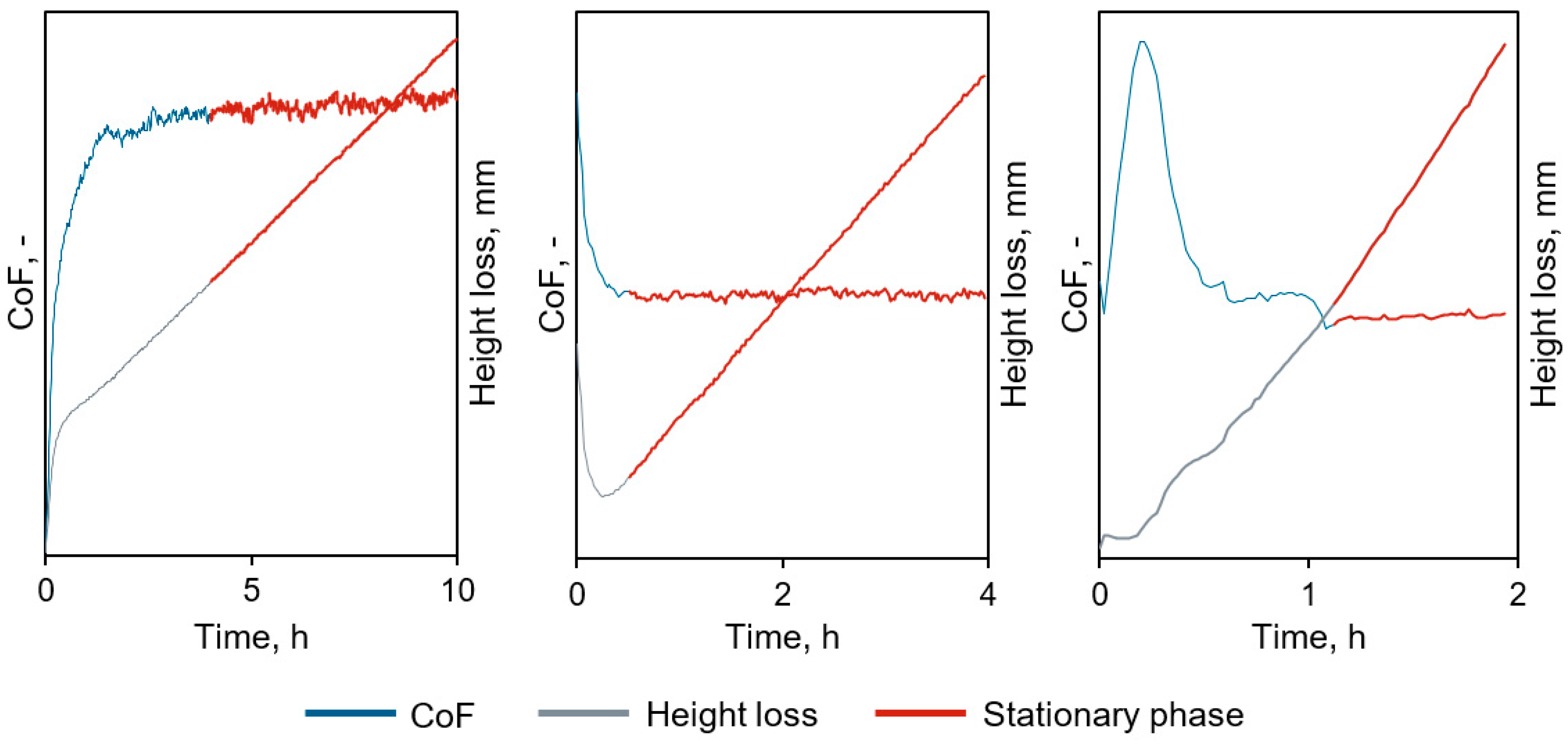
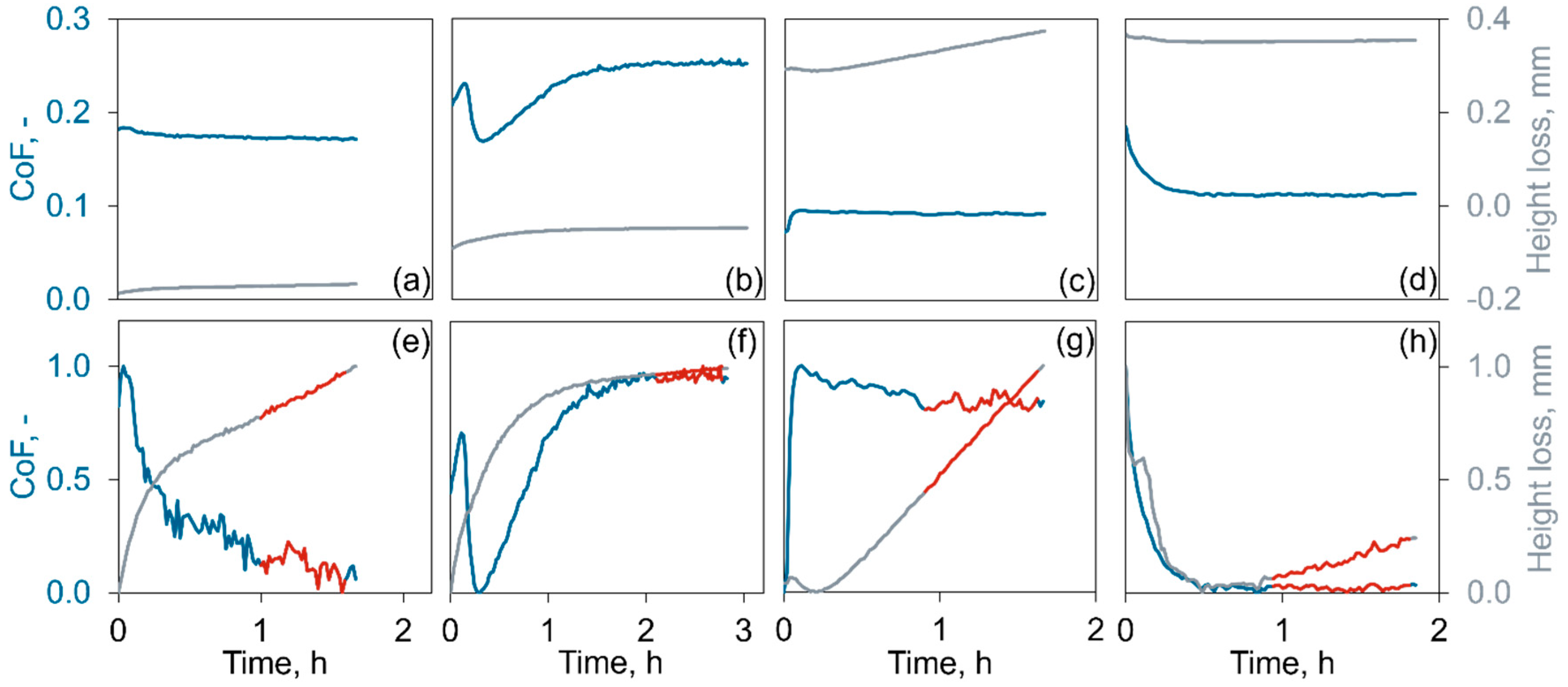
However, with different tribological materials and test conditions, such as load spectra, the data obtained from tribological measurements show distinct time patterns and significant short-term fluctuations (see
Figure 2). Consequently, it becomes more than challenging to reliably determine the stationary phase using straightforward mathematical methods, such as calculating the first derivative.
As a result, the identification of the stationary phase in the subsequent data processing of all tribological tests in currently performed manually. Furthermore, due to the lack of a clear mathematical definition and standard for the stationary phase, different individuals may have different interpretations of the same experiment’s stationary. Such tasks, which lack a clear definition, are precisely where artificial neural networks thrive.
In the domain of neural network applications, problems involving the analysis of data patterns are often categorized under image recognition or image processing. This category is well-suited for Convolutional Neural Networks (CNNs) due to their effectiveness in handling two-dimensional image data [
25,
26,
27,
28]. However, unlike typical two-dimensional images, experimental curves from tribological tests are one-dimensional and lack RGB color information. These curves are inherently time-dependent, capturing variations over a continuous time scale. Thus, in the context of neural network tasks, this problem should be categorized under time series data classification rather than image processing. Compared to CNNs, Long Short-Term Memory networks (LSTMs) are highly effective in capturing long-term dependencies within time series data and retaining essential information. This capability allows LSTMs to establish connections over extended periods and to handle data of varying lengths more flexibly and efficiently [
29,
30,
31,
32]. Consequently, LSTMs are better suited for identifying the stationary phase in tribological experiment data.
2.2. Long Short-Term Memory Network Structure
2.2.1. LSTM Cell and Cell State
The concept of LSTM network was first introduced by Sepp Hochreiter and Jürgen Schmidhuber in 1997 to address the limitations of traditional recurrent neural networks (RNNs) in handling long-term dependencies [
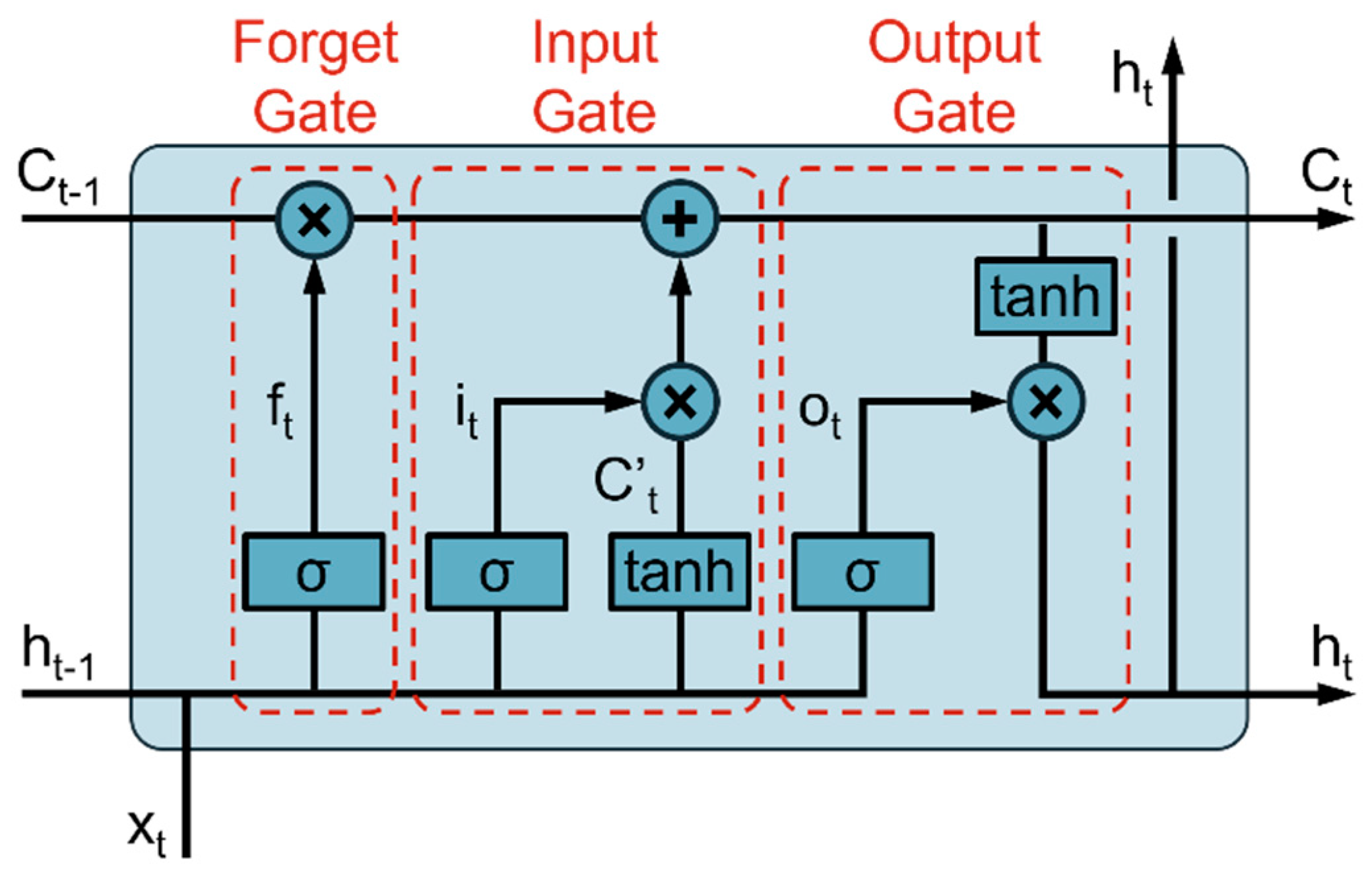
29]. Traditional RNNs suffer from the vanishing or exploding gradient problems, which make them inefficient for learning from data with long-range temporal dependencies. LSTM networks were designed to overcome these issues by introducing a more complex architecture capable of learning and retaining information over extended periods. LSTM networks extend the architecture of standard RNNs by incorporating a memory cell, which is capable of maintaining its state over long sequences. The core of the LSTM architecture is the cell state, which is regulated by three main components called gates: the input gate, the forget gate, and the output gate. These gates control the flow of information into, out of, and through the cell state, allowing the network to selectively remember or forget information (
Figure 3).
The forget gate f
t determines which information from the previous cell state (Long-Term Memory) C
t-1 should be forgotten. It is computed by applying a sigmoid function σ to the weighted sum of the previous hidden state (Short-Term Memory) h
t-1 and the current input x
t, plus a bias b
f:
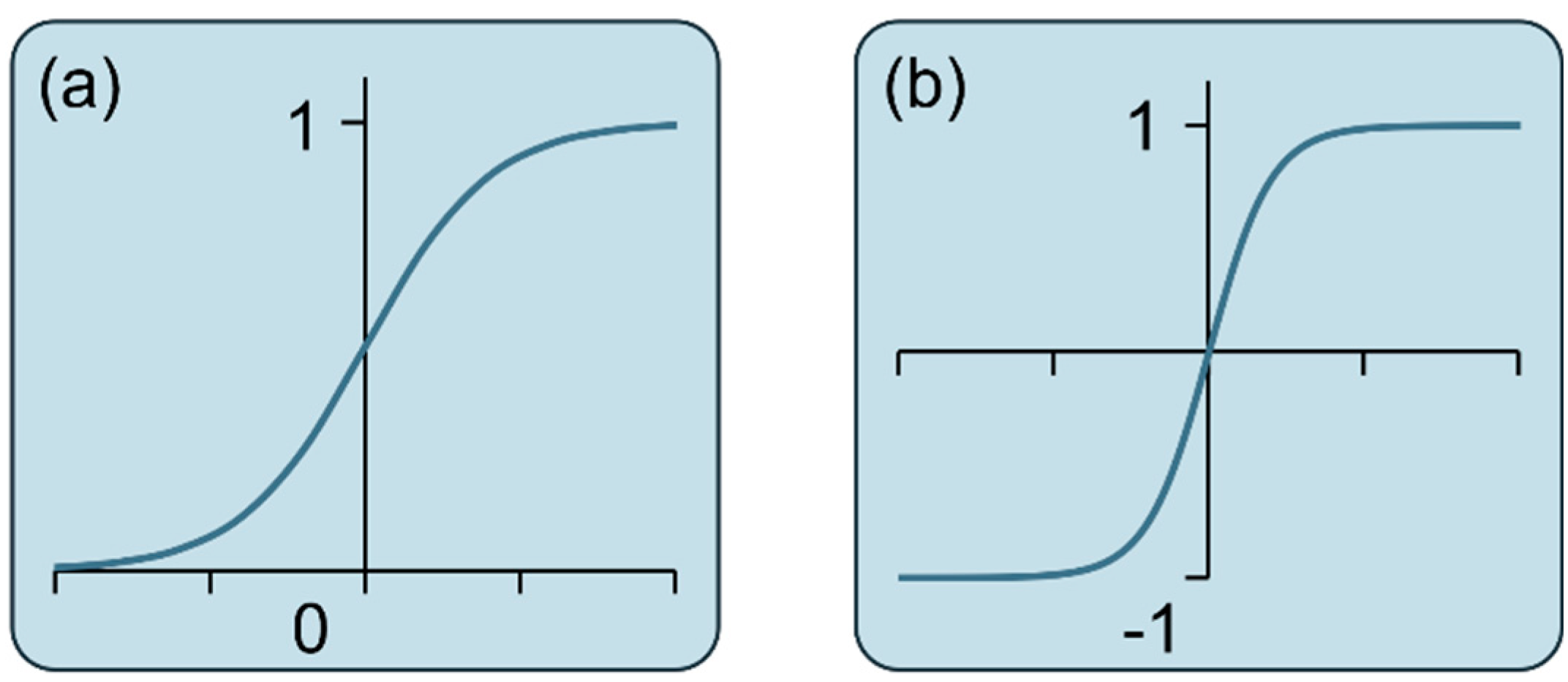
The sigmoid (σ) function squashes the input to a value between 0 and 1, allowing the forget gate to control the extent to which information is retained or discarded. It is defined as (
Figure 4a):
The input gate i
t controls the amount of new information to be added to the cell state. It is calculated similarly to the forget gate using a sigmoid function. The candidate cell state C’
t, which represents the new information to be added, is computed using a hyperbolic tangent (tanh) function that scales the input to a value between -1 and 1:
The tanh function squashes the input to a value between -1 and 1, providing a normalized range for the candidate cell state. It is defined as (
Figure 4b):
The cell state C
t is then updated by combining the previous cell state C
t-1 scaled by the forget gate f
t and the candidate cell state C’
t scaled by the input gate i
t:
The output gate o
t determines the output of the LSTM cell. It is computed by applying a sigmoid function to the weighted sum of the previous hidden state h
t-1 and the current input x
t, plus a bias b
o. The hidden state h
t is then calculated by applying a tanh function to the updated cell state C
t and scaling it by the output gate o
t:
The primary advantage of LSTM networks lies in their ability to maintain long-term dependencies by preserving gradients across many timesteps. This capability is made possible through the forget gate f
t, which controls the extent to which information from the previous cell state C
t-1 is retained. Mathematically, the gradient of the cell state can be expressed as:
Since the forget gate ft is typically close to 1, the gradient remains substantial over time, effectively mitigating the vanishing gradient problem that plagues traditional RNNs. This allows the network to maintain and learn from long-term dependencies in time series data. Therefore, LSTM networks address the fundamental limitations of traditional RNNs, particularly in tasks involving extended temporal sequences Their architecture, characterized by memory cells and gating mechanisms, equips them to handle complex temporal patterns effectively, making them a powerful tool for a wide array of sequence learning applications.
2.2.2. LSTM Network Architecture
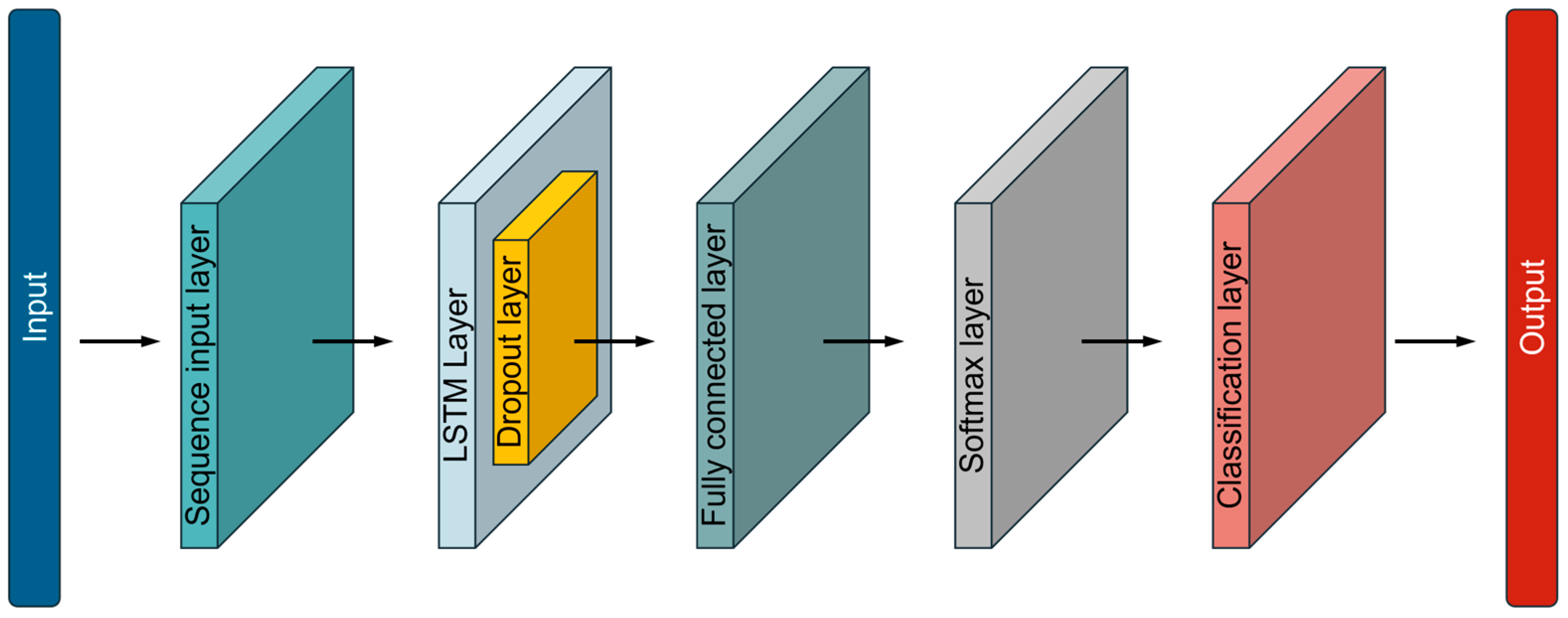
The proposed LSTM network architecture is a structured sequence of layers specifically designed to process and classify time series data, leveraging the strengths of Long Short-Term Memory (LSTM) networks (
Figure 5). This architecture is composed of several essential layers, each serving a distinct function within the overall model. The network begins with a
sequence input layer. This is crucial as it forms the entry point for sequential data, allowing the model to process inputs with varying lengths and multiple features, which in this study, are CoF and height loss. The sequence input layer ensures that the network is adaptable to different types of time series data, making it well-suited for tasks such as analyzing CoF, height loss, and other possible time-dependent tribological phenomena. Central to the architecture is the
LSTM layer, which is the heart of the network. The LSTM layer is designed to capture both short-term fluctuations and long-term trends in the data through its unique cell structure and gating mechanisms. Enabling the network to effectively retain important information over extended sequences. To prevent overfitting, which is a common challenge in deep learning models, a
dropout layer is incorporated into the architecture. The dropout layer functions as a regularization technique, randomly deactivating a subset of neurons during the training process. This prevents the network from becoming too specialized to the training data and enhances its ability to generalize to new, unseen data. By reducing the risk of overfitting, the dropout layer contributes to the robustness and reliability of the model’s predictions. Following the LSTM and dropout layers is the
fully connected layer, also known as the dense layer. This layer acts as an integrator, combining the high-level features extracted by the LSTM layer into a format suitable for classification. The fully connected layer serves as a bridge between the learned temporal features and the output classes, making it a critical component for mapping the extracted information to specific categories. The final stages of the network include the
softmax layer and the
classification layer. The softmax layer converts the outputs from the fully connected layer into a probability distribution over the classes. This probability distribution allows the model to assign confidence levels to each class, indicating how likely the input sequence belongs to each possible category. The classification layer then takes this probabilistic output and makes the final decision, selecting the class with the highest probability as the predicted label. This LSTM-based architecture is designed to handle complex time series data effectively, leveraging the strengths of LSTM networks for sequence modeling. The combination of memory capabilities, regularization techniques, and robust classification layers makes this network well-equipped for a variety of sequential data tasks. The design not only captures intricate temporal patterns but also ensures that the model remains generalizable and resistant to overfitting.
2.2.3. Training Data Preparation
In preparation for training the LSTM network, extensive work was carried out on the data, ensuring that it was suitably structured for effective model learning. Data were selected from a wide range of previous tribological experiments, specifically focusing on tests involving polymer-based tribocomposites and steel counterparts. Polymer-based tribocomposites were chosen due to their excellent self-lubricating properties, which facilitate the formation of transfer films on the surface of counterpart under various experimental conditions, thereby stabilizing the friction coefficient and reducing wear rate [
33,
34]. The dataset encompasses a diverse array of conditions, including varying tribomaterials, load conditions, experimental temperatures and test durations. This diversity in the data was crucial to capturing the full spectrum of tribological behaviors, thereby enhancing the generalizability of the neural network [
35,
36,
37]. Given that the experimental data was processed by different researchers, the dataset inherently reflects variations in the judgment of stationary phase during the tribological tests. This variability is advantageous for the neural network as it introduces a level of complexity that fosters the development of robust, generalizable models capable of interpreting a wide range of stationarity criteria.
To efficiently handle the data, a custom script was developed to automatically label each data point according to the stationary phase identified by the researchers during their analysis. The script categorizes all data points into two classes: “stationary” and “other”. This binary classification simplifies the data and ensures that the neural network can focus on learning the critical distinctions between stationary and running-in phases. Additionally, all data was normalized along the Y-axis to a range oof 0 to 1 (
Figure 6). This normalization step is essential as it accelerates the convergence of the neural network during training, improves model stability, and enhances generalization. However, the X-axis (time-axis) was deliberately left unnormalized. Given the LSTM network’s inherent ability to manage sequences of varying lengths, normalizing the time axis could potentially obscure temporal patterns that are vital for accurate feature extraction.
In total, 3364 datasets were prepared for training, with experiment durations ranging from 0.5 hours to 19 hours, although most experiments lasted less than 5 hours. This comprehensive data preparation ensures that the LSTM network is well-equipped to learn from a diverse set of conditions, thereby enhancing its ability to generalize across different tribological scenarios.
2.2.4. Hyperparameters Optimization
The performance of Long Short-Term Memory networks, as well as other types of neural networks, is heavily influenced by the choice of hyperparameters. Hyperparameters, such as the number of layers, the number of neurons in each layer, learning rate, dropout rate, and mini batch size, play a crucial role in determining the model’s ability to learn from data and generalize to unseen data. Selecting optimal hyperparameters is a crucial task due to the vast search space and the complex interactions between different parameters. In hyperparameter optimization, the goal is to find the set of hyperparameters that minimizes or maximize a specific objective function, typically a measure of model performance like validation accuracy or loss. Several methods exist for hyperparameter optimization, including grid search, random search, and more advanced techniques like Bayesian optimization. In this study, Bayesian optimization was employed for hyperparameter tuning due to its efficiency in exploring the hyperparameter space with fewer evaluations compared to traditional methods. Unlike grid search, which exhaustively searches the entire space, or random search, which samples the space randomly, Bayesian optimization uses probabilistic models to predict the performance of hyperparameter configurations. This allows it to focus the search on promising regions of the hyperparameter space, thereby reducing the computational cost.
At the heart of Bayesian optimization lies the construction of a surrogate model to approximate the true objective function. The surrogate model, most commonly a Gaussian Process (GP), models the objective function as a distribution over possible functions, with any finite set of function values following a multivariate normal distribution. This allows the GP to provide a mean prediction of the objective function at any point (here means a certain combination of hyperparameters) in the hyperparameter space, along with a corresponding uncertainty or variance . This dual capability is crucial for making informed decisions about where to evaluate the objective function next, thereby optimizing the process.
This dual capability is crucial for making informed decisions about where to evaluate the objective function next, thereby optimizing the process [
38]. Given the vast number of hyperparameters and the exponential growth in the number of possible combinations, the challenge in hyperparameter optimization lies in efficiently exploring this high-dimensional space. The goal of Bayesian optimization is to find the optimal configuration within a limited number of evaluations, as evaluating every possible combination is computationally infeasible. To achieve this, the optimization process begins with evaluating the objective function at a set of initial points, known as seed points, which are selected either randomly or based on prior knowledge. They provide the Gaussian Process with a broad initial understanding of the hyperparameter space, enabling the model to start building a surrogate that can effectively guide the search towards promising regions. A critical component to Bayesian optimization is the acquisition function, which guides the selection of the next point
in the hyperparameter space to evaluate. In this study, the Expected Improvement (EI) acquisition function was employed. The EI function is defined as:
where
is the best observed value of the objective function so far, and
is the predicted value at a new point. The EI function balances the need to explore regions of the hyperparameter space where the GP’s predictions are uncertain (exploration) with the need to refine known good regions (exploitation). By maximizing the EI, the optimization process avoids getting trapped in local minima, a common issue in high-dimensional spaces and systematically improves the objective function. After evaluating the new point
, the result is used to update the GP, refining the surrogate model’s predictions. This iterative process continues until a predefined stopping criterion is met, such as a maximum number of evaluations or when improvements become negligible [
39,
40]. In this study, the optimization was conducted over 100 evaluations, allowing the model to progressively converge toward an optimal hyperparameter configuration. Considering the total evaluations of 100, the number of seed points was set to be 30, ensuring that the initial exploration phase was sufficiently broad to capture diverse regions of the hyperparameter space before the model began to focus on refining the search in subsequent iterations.
During the optimization, each evaluation of the surrogate model involves training the network with a specific set of hyperparameters and assessing its performance. However, the training process for neural networks is inherently stochastic, meaning that even with the same set of hyperparameters, the resulting model performance can vary significantly due to factors such as random initialization of weights and the stochastic nature of gradient descent. This variability can make it difficult to accurately evaluate the true performance of a given hyperparameter configuration. To mitigate the impact of this randomness and obtain a more reliable estimate of model performance, K-fold cross-validation was employed. K-fold cross-validation divides the data into K subsets and performs training and validation K times, each time using a different subset as the validation set and the remaining subsets as the training set. By averaging the validation results across all folds, this approach provides a robust estimate of model performance, reducing the risk of overfitting to any single data split. To reduce the impact of randomness in training and avoid the excessive time costs associated with repeated training, the K-value was set to 5. All 3364 data samples were randomly split into two sets: 3350 samples were allocated for training and validation, and 14 samples were reserved for testing. This division aimed to ensure that a sufficient amount of data was available for training and validation, which is crucial for preventing overfitting, while retaining a small portion of the data for testing to verify the network’s generalizability. Based on this strategy, the objective function in the Bayesian optimization process was defined as the reciprocal of weighted average of validation accuracy and test accuracy, with weights of 0.6 and 0.4, respectively, as defined by the following equation:
where
is the objective (network performance),
stands for validation accuracy and
stands for test accuracy. Thus, throughout the Bayesian optimization process, a total of 100 hyperparameter configurations were evaluated. Each configuration was subjected to K-fold cross-validation, where the network was trained and evaluated five times. The mean value of objective across these five evaluations was used as the final performance metric for each hyperparameter configuration. The configuration with the lowest objective was selected as the optimal set of hyperparameters.
2.2.5. LSTM-Network Optimization
As mentioned in former chapter, the training of neural networks is inherently stochastic. Therefore, after selecting the optimal hyperparameter configuration via Bayesian optimization, we conducted 500 additional training runs on the LSTM network using the same training dataset. This extensive training was designed to reduce or mitigate the randomness inherent in the training process, allowing us to identify the network with the best performance. The evaluation of the network’s performance was not solely relied upon the validation accuracy and test accuracy, which was defined as the percentage of correctly labeled data out of the total number of data points. Additionally, the friction coefficient and specific wear rate values identified by the LSTM network during the stable phase were calculated as
and
and then compared with the corresponding values derived from manually processed data by the researchers, denoted as
and
. The relative error between these values was computed as defined by the following equation:
where
represents the relative error, and
represents either the friction coefficient (
) or the specific wear rate (
). This approach was employed to ensure that the network trained through this entire process could be used effectively as a replacement for manual data processing, enabling rapid and efficient batch processing of experimental data.
3. Results and Discussion
3.1. Chosen Hyperparameter from Bayesian Optimization
In accordance with the methods described in Chapter 2, several hyperparameters that significantly impact the training of LSTM networks were selected as optimized variables. These included the number of LSTM layers, the number of neurons per layer, Dropout Rate, Initial Learning Rate, Learning Rate Drop Factor, Learning Rate Drop Period, and MiniBatch Size. To ensure that the parameters are chosen within a sufficiently broad range while balancing the time and computational resources required, these hyperparameters were optimized within their predefined ranges. For example, considering the data volume, the number of feature variables, and the complexity of the data, the number of LSTM layers was limited to either one or two, with the number of neurons per layer constrained between 50 and 150, among other settings. The selection of these hyperparameter ranges was not arbitrary but was determined based on the specific task requirements, data volume, training strategies, and the experience of the researchers. The optimized hyperparameters and their respective ranges used in this study are summarized in
Table 1.
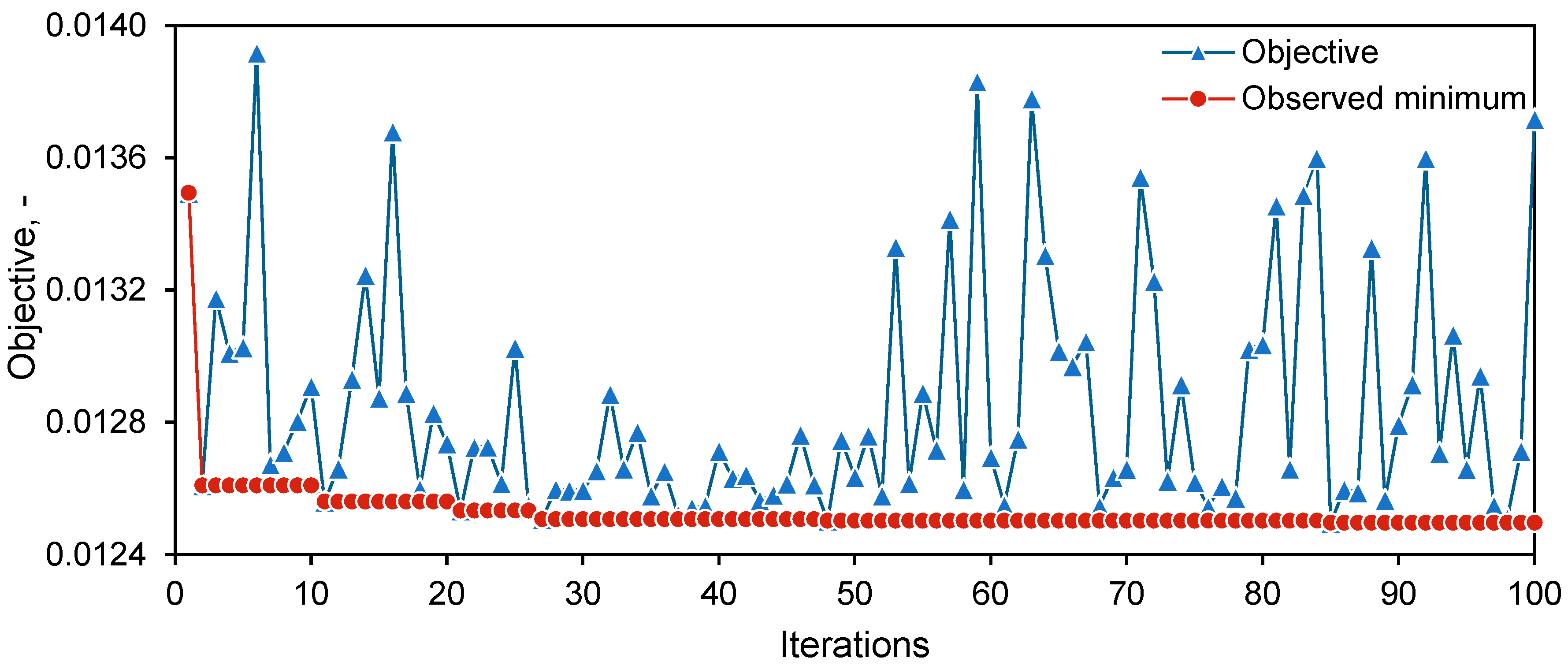
After nearly 29 hours and 500 evaluations of the LSTM network, the 85
th hyperparameter configuration was identified as the optimal result obtained so far. The 100 objectives and observed minimums throughout the optimization process are illustrated in
Figure 7. As depicted, Bayesian optimization not only focuses on exploring the known optimum by selecting nearby points but also intermittently explores unknown regions of the hyperparameter space. This strategy is designed to search for potential global optima and avoid getting trapped in local minima. Additionally, the range of results from the first 30 randomly selected hyperparameter configurations already encompasses most of the range observed throughout the entire optimization process. This suggests that these 30 random points broadly constructed the surrogate model over the hyperparameter space.
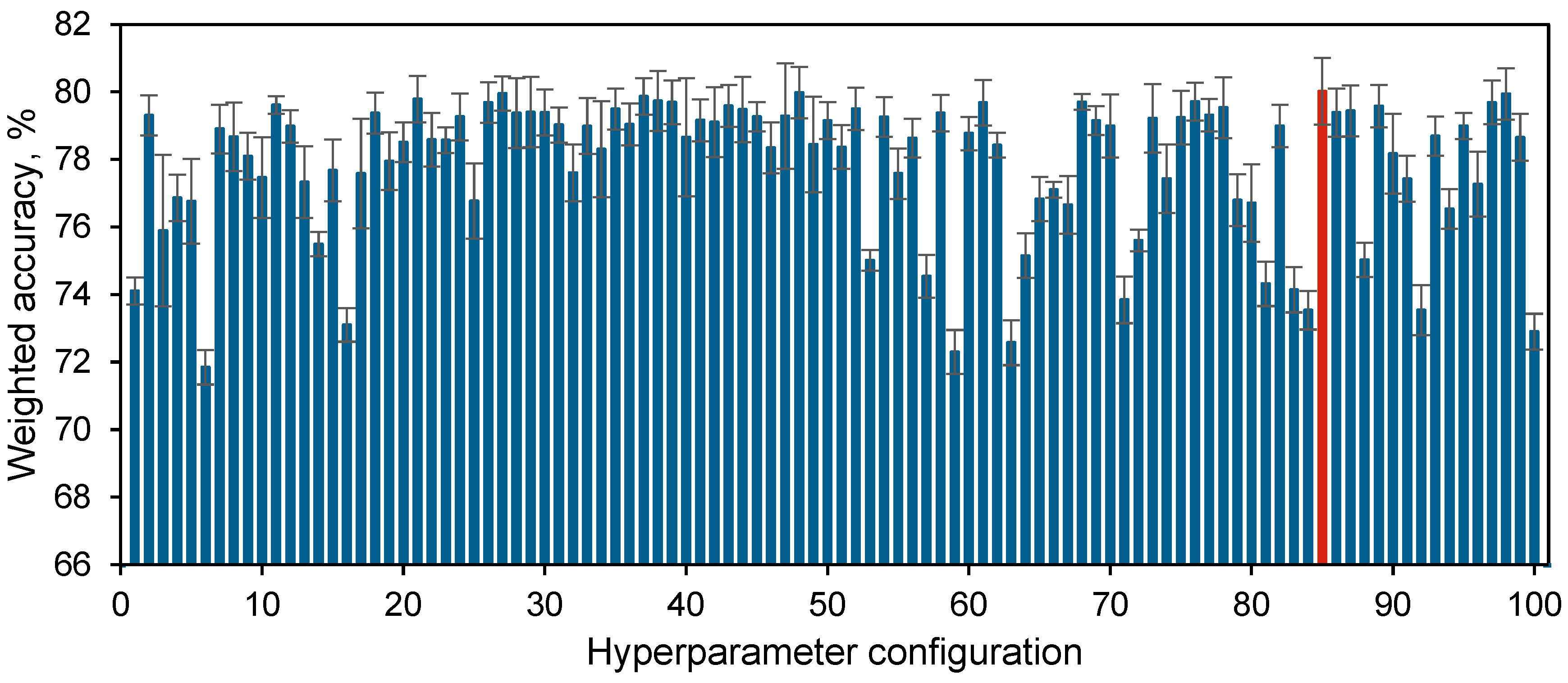
Figure 8 illustrates the weighted average accuracy of each hyperparameter configuration corresponding to the Bayesian optimization objectives. It is evident that the LSTM network trained with the 85
th hyperparameter configuration (marked in red) achieved a weighted average accuracy of 80.02%, with an average validation accuracy of 80.44% and an average test accuracy of 79.38%. Additionally, it can be observed that different hyperparameter configurations significantly impact the network’s performance. For instance, some configurations resulted in network accuracy as low as 70%, nearly 10% lower than the optimal solution, which would have a substantial impact on the final prediction results.
The values of this optimized hyperparameter set are listed in
Table 2. These specific hyperparameter means, that this optimized LSTM network consists of one LSTM layer (Number of layers = 1) with 59 neurons (Number of neurons per layer = 59). During each iteration, 10.2% of the LSTM layer’s neurons (Dropout Rate = 0.0102) were deactivated to prevent overfitting. The initial learning rate was set to 0.0097 (Initial Learning Rate = 0.0097), and after every 18 epochs (Learning Rate Drop Period = 18), the learning rate was reduced to 60.07% of its previous value (Learning Rate Drop Factor = 0.6007). Additionally, each iteration used 16 data samples (MiniBatch Size = 16) for training the network. In summary, the entire network training process was defined and shaped by these hyperparameter.
3.2. LSTM-Network Training
After the hyperparameter configuration was selected through Bayesian optimization, the LSTM network training process defined by this configuration was repeated 500 times to reduce the impact of randomness on the training results.
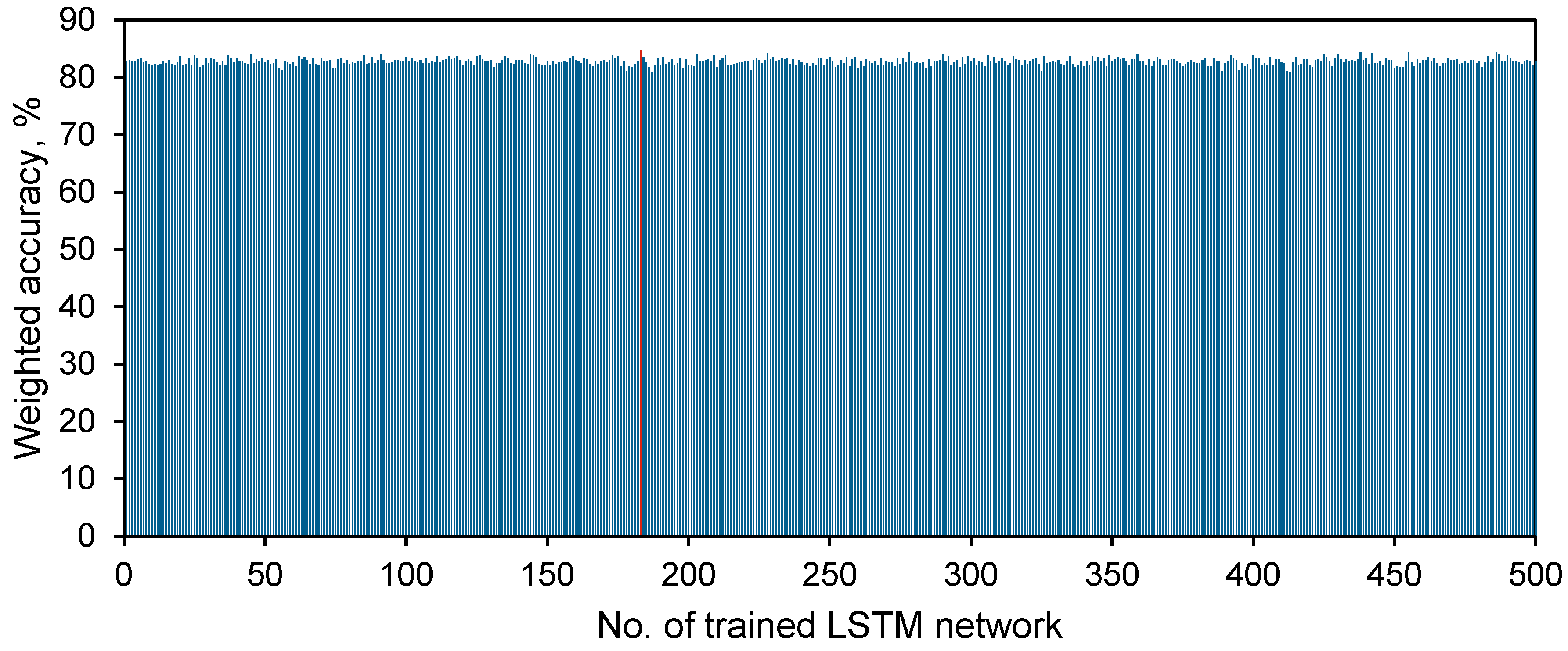
Figure 9 illustrates the weighted accuracy of all 500 trained networks. The training data and network performance evaluation methods used were consistent with those employed during the Bayesian optimization process. As shown in the figure, even when affected by the inherent randomness of training, the network's performance remained relatively stable, with all networks achieving a weighted accuracy above 80%. This demonstrates that the strong performance of this hyperparameter configuration during Bayesian optimization was not merely a result of fortunate randomness but indeed positively influenced the network training outcome. Ultimately, the network trained during the 183rd iteration (marked in red) was selected as the final model, achieving a weighted average accuracy of 84.64%, with validation and test accuracies of 83.18% and 86.83%, respectively.
As mentioned in Chapter 2, accuracy is defined as the ratio of correctly classified data points to the total number of data points. While this parameter reflects the LSTM network's performance in data classification, it does not fully capture the practical significance of the data processing, specifically, how closely the data processed by the LSTM network resembles the data processed manually by researchers, and how different the resulting CoF and w
s. To address this, the results of the 14 test data sets identified by the trained LSTM network were specifically visualized and analyzed, and the CoF and w
s derived from these results were calculated.
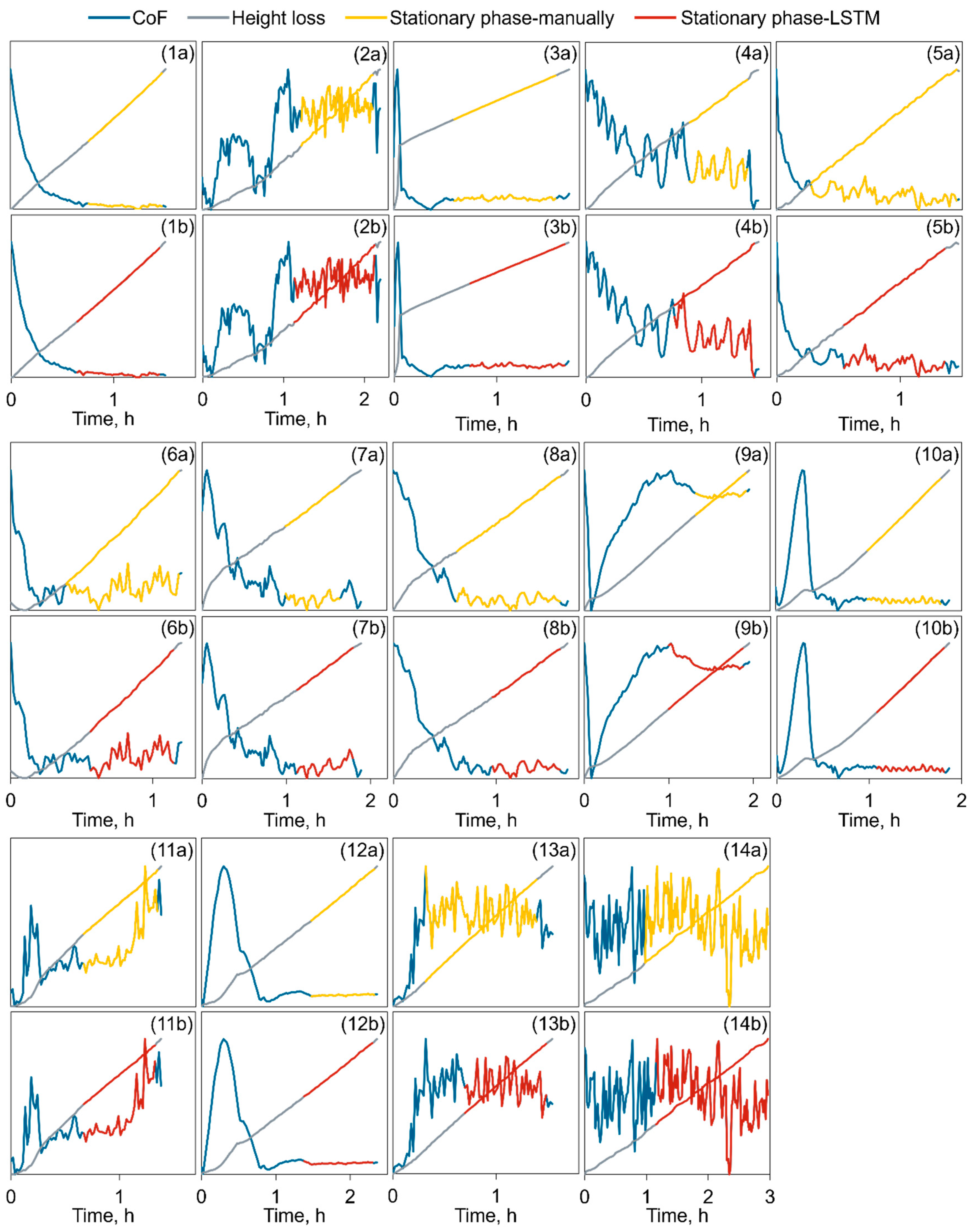
Figure 10 presents the stationary phase identified by both the researchers and the LSTM network for all 14 test data sets. The comparison shows that, although there are slight differences between the LSTM network's selections and those made manually, the LSTM network's choices are largely consistent with the definition of a stationary phase, with some even being more reasonable than the manual selections.
Correspondingly, the CoF and w
s calculated from the stationary phases identified by the LSTM network were compared with those manually computed by the researchers.
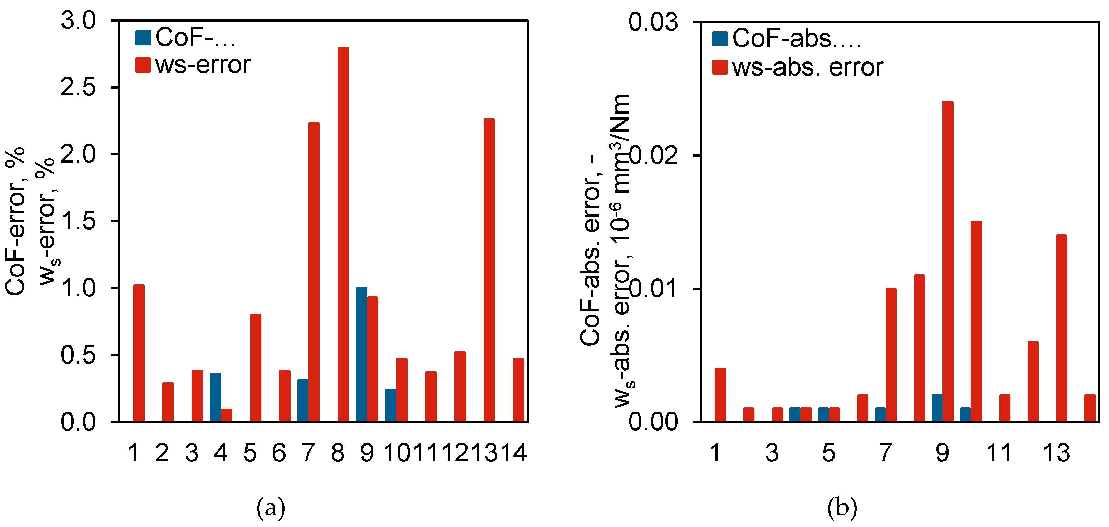
Figure 11 illustrates the differences between these two sets of values, including both the percentage differences and the absolute differences. As shown in the diagram, the discrepancies between the results identified by the LSTM network and those processed by the researchers are minimal. This is particularly evident in the CoF, where the highest percentage difference is merely 1% (
Figure 11a), corresponding to an absolute difference of just 0.002 (
Figure 11b). Given that friction coefficients are typically measured with precision only to two decimal places, this difference is practically negligible. For w
s, the error is slightly higher than that for CoF, but the maximum percentage difference is still only 2.79%, with a corresponding absolute difference of 0.024.
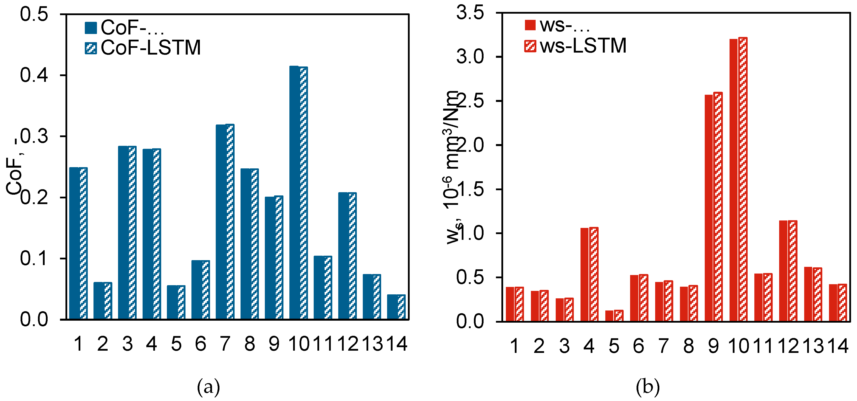
When directly comparing the CoF and w
s identified by the LSTM network with those determined manually, the values are almost identical (
Figure 12). This suggests that a well-trained LSTM network, developed using appropriate methodologies, can effectively identify the stationary phases in tribological experiment data, serving as a viable alternative to manual analysis and data processing.
4. Conclusion
In this study, we developed and optimized an LSTM network specifically designed for analyzing time-series data and identifying stationary phases in tribological experiment datasets. Through the application of Bayesian optimization, we systematically fine-tuned several critical hyperparameters, including the number of LSTM layers, neurons per layer, dropout rate, and learn rate parameters. This approach led to the discovery of an optimal configuration, significantly improving the network's ability to accurately process the data.
The results were promising, with the optimized LSTM network demonstrating robust performance. It achieved a weighted average accuracy of 84% across various training iterations. The differences observed between the stationary phases detected by the LSTM and those determined manually were minimal, with the friction coefficient (CoF) showing a maximum discrepancy of 1%, and the specific wear rate (ws) displaying similar discrepancies. The LSTM network's ability to identify CoF and ws values that were nearly identical to those calculated manually further emphasized its precision and reliability.
Moreover, the combination of Bayesian optimization and K-fold cross-validation effectively reduced the impact of training randomness and ensured that the selected hyperparameters were generalizable across different data subsets. This integrated strategy provided a reliable method for optimizing the network while maintaining the stability and consistency of the results.
In summary, our study demonstrates that a well-trained and optimized LSTM network can serve as a dependable instrument for automating the detection of stationary phases from tribological data determined in experiments. This method facilitates the effective and accurate extraction of conclusions from the measured data, making it invaluable for the reliable assessment of tribological systems and in the realm of material development.
Acknowledgments
We acknowledge the German Research Foundation (DFG) for the financial support of the research through grant 399606374.
References
- Jones, S.P.; Jansen, R.; Fusaro, R.L.: Preliminary investigation of neural network techniques to predict tribological properties. Tribology Transactions 40(2), 312–320, 1997. [CrossRef]
- Jiang, Z.; Zhang, Z.; Friedrich, K.: Prediction on wear properties of polymer composites with artificial neural networks. Composites Science and Technology 67(2), 168–176, 2007. [CrossRef]
- Zhang, Z.; Friedrich, K.; Velten, K.: Prediction on tribological properties of short fibre composites using artificial neural networks. Wear 252(7–8), 668–675, 2002. [CrossRef]
- Zhang, Z.; Klein, P.; Friedrich, K.: Dynamic mechanical properties of PTFE based short carbon fibre reinforced composites: Experiment and artificial neural network prediction. Composites Science and Technology 62(7–8), 1001–1009, 2002. [CrossRef]
- Zhang, Z.; Barkoula, N.M.; Karger-Kocsis, J.; Friedrich, K.: Artificial neural network predictions on erosive wear of polymers. Wear 255(1–6), 708–713, 2003. [CrossRef]
- Gyurova, L.A.; Friedrich, K.: Artificial neural networks for predicting sliding friction and wear properties of polyphenylene sulfide composites. Tribology International 44(5), 603–609, Elsevier, 2011. [CrossRef]
- Gao, G.; Gong, J.; Qi, Y.; et al.: Tribological Behavior of PTFE Composites Filled with PEEK and Nano-ZrO2. Tribology Transactions 63(2), 296–304, Taylor & Francis, 2020. [CrossRef]
- Zakaulla, M.; Parveen, F.; Amreen; Harish; Ahmad, N.: Artificial neural network based prediction on tribological properties of polycarbonate composites reinforced with graphene and boron carbide particle. Materials Today: Proceedings 26, 296–304, Elsevier Ltd., 2019. [CrossRef]
- Velten, K.; Reinicke, R.; Friedrich, K.: Wear volume prediction with artificial neural networks. Tribology International 33(10), 731–736, 2000. [CrossRef]
- Jiang, Z.; Gyurova, L.; Zhang, Z.; Friedrich, K.; Schlarb, A.K.: Neural network based prediction on mechanical and wear properties of short fibers reinforced polyamide composites. Materials and Design 29(3), 628–637, 2008. [CrossRef]
- Jiang, Z.; Gyurova, L.A.; Schlarb, A.K.; Friedrich, K.; Zhang, Z.: Study on friction and wear behavior of polyphenylene sulfide composites reinforced by short carbon fibers and sub-micro TiO2 particles. Composites Science and Technology 68(3–4), 734–742, 2008. [CrossRef]
- Gyurova, L.A.; Miniño-Justel, P.; Schlarb, A.K.: Modeling the sliding wear and friction properties of polyphenylene sulfide composites using artificial neural networks. Wear 268(5–6), 708–714, 2010. [CrossRef]
- Gyurova, L.; Jiang, Z.; Schlarb, A.K.; Friedrich, K.; Zhang, Z.: Study on the Wear and Friction of Short Carbon Fiber and/or Nano-TiO2 Reinforced Polyphenylene Sulfide Composites using Artificial Neural Networks. Friction, Wear and Wear Protection 417–422, 2009. [CrossRef]
- Busse, M.; Schlarb, A.K.: A novel neural network approach for modeling tribological properties of polyphenylene sulfide reinforced on different scales. Tribology of Polymeric Nanocomposites: Friction and Wear of Bulk Materials and Coatings: Second Edition 779–793, 2013. [CrossRef]
- Zhao, Y.; Lin, L.; Schlarb, A.K.: Artificial neural network accomplished prediction on tribology – A promising procedure to facilitate the tribological characterization of polymer composites. Wear 532–533(May), 205106, Elsevier B.V., 2023. [CrossRef]
- Frangu, L.; Ripa, M.; Multi, I.I.; Perceptron, L.: Artificial Neural Networks Applications in Tribology – A Survey. Construction (October), 2001.
- Sose, A.T.; Joshi, S.Y.; Kunche, L.K.; Wang, F.; Deshmukh, S.A.: A review of recent advances and applications of machine learning in tribology. Physical Chemistry Chemical Physics 25(6), 4408–4443, 2023. [CrossRef]
- Paturi, U.M.R.; Palakurthy, S.T.; Reddy, N.S.: The Role of Machine Learning in Tribology: A Systematic Review. Springer Netherlands, 2023. [CrossRef]
- Zhang, Z.; Friedrich, K.: Artificial neural networks applied to polymer composites: A review. Composites Science and Technology 63(14), 2029–2044, 2003. [CrossRef]
- Aiordachioaie, D.; Ceanga, E.; Roman, N.; Mihalcea, R.: Pre-processing of acoustic signals by neural networks for fault detection and diagnosis of rolling mill. (440), 7–9, 1997.
- Yin, F.; He, Z.; Nie, S.; Ji, H.; Ma, Z.: Tribological properties and wear prediction of various ceramic friction pairs under seawater lubrication condition of different medium characteristics using CNN-LSTM method. Tribology International 189(July), 108935, Elsevier Ltd, 2023. [CrossRef]
- Yin, F.; Luo, H.; Nie, S.; Ji, H.; Ma, Z.: Physics-Informed machine learning for tribological properties prediction of S32750/CFRPEEK tribopair under seawater lubrication via PISSA-CNN-LSTM. Tribology International 199(June), 109965, Elsevier Ltd, 2024. [CrossRef]
- Motamedi, N.: Towards the prediction and understanding of To cite this version : 2023.
- o. A.: DIN ISO 7148-2:2014-07. Gleitlager - Prüfung des tribologischen Verhaltens von Gleitlagerwerkstoffen - Teil 2: Prüfung von polymeren Gleitlagerwerkstoffen (ISO 7148-2:2012) 2014.
- LeCun, Y.; Boser, B.; Denker, J.S.; et al.: Backpropagation Applied to Handwritten Zip Code Recognition. Neural computation 1(4), 541–551, 1989. [CrossRef]
- LeCun, Y.; Bottou, L.; Bengio, Y.; Haffner, P.: Gradient-Based Learning Applied to Document Recognition. Proceedings of the IEEE 86(11), 2278–2324, 1998. [CrossRef]
- Platt, J.C.; Nowlan, S.J.: A convolutional neural network hand tracker. Proc. Adv. Neural Inf. Process. Sys 901–908, 1995.
- Lawrence, S.; Giles, C.L.; Tsoi, A.C.; Back, A.D.: Face Recognition: A Convolutional Neural-Network Approach. IEEE transactions on neural networks 8(1), 98–113, 1997. [CrossRef]
- Hochreiter, S.; Schmidhuber, J.: Long Short-Term Memory. Neural computation 9(8), 1735–1780, 1997. [CrossRef]
- Karim, F.; Majumdar, S.; Darabi, H.; Chen, S.: LSTM Fully Convolutional Networks for Time Series Classification. IEEE Access 6(c), 1662–1669, 2017. [CrossRef]
- Karim, F.; Majumdar, S.; Darabi, H.: Insights into lstm fully convolutional networks for time series classification. IEEE Access 7, 67718–67725, IEEE, 2019. [CrossRef]
- Sadouk, L.: CNN Approaches for Time Series Classification. Time Series Analysis - Data, Methods, and Applications 1–23, 2019. [CrossRef]
- Zhao, S.; Hua, C.; Zhao, Y.; Sun, C.; Lin, L.: Casting of regulable nanostructured transfer film by detaching nanofiller from the composite into the tribosystem – A strategy to customize tribological properties. Tribology International 195(March), 109597, Elsevier Ltd, 2024. [CrossRef]
- Zhao, Y.; Lin, L.: Dependence of the tribological performance of PEEK-based sustainable composites on the temperature. Materials Today Sustainability 25(October 2023), 100625, Elsevier Ltd, 2024. [CrossRef]
- Chong, S.Y.; Tiňo, P.; Yao, X.: Relationship between generalization and diversity in coevolutionary learning. IEEE Transactions on Computational Intelligence and AI in Games 1(3), 214–232, 2009. [CrossRef]
- Yang, J.; Zeng, X.; Zhong, S.; Wu, S.: Effective neural network ensemble approach for improving generalization performance. IEEE Transactions on Neural Networks and Learning Systems 24(6), 878–887, 2013. [CrossRef]
- Ortega, L.A.; Cabañas, R.; Masegosa, A.R.: Diversity and Generalization in Neural Network Ensembles. Proceedings of Machine Learning Research 151, 11720–11743, 2022.
- Mockus, J.: The Bayesian Approach to Global Optimization. In Springer Science and Business Media, 1981.
- Pelikan, M.; Goldberg, D.E.; Cantú-Paz, E.: Hierarchical problem solving by the Bayesian optimization algorithm. In Proceedings of the 2nd Annual Conference on Genetic and Evolutionary Computation, 2000.
- Pelikan, M.; Goldberg, D.E.: Research on the Bayesian Optimization Algorithm. IlliGAL Report (2000010), 2000.
|
Disclaimer/Publisher’s Note: The statements, opinions and data contained in all publications are solely those of the individual author(s) and contributor(s) and not of MDPI and/or the editor(s). MDPI and/or the editor(s) disclaim responsibility for any injury to people or property resulting from any ideas, methods, instructions or products referred to in the content. |
© 2024 by the authors. Licensee MDPI, Basel, Switzerland. This article is an open access article distributed under the terms and conditions of the Creative Commons Attribution (CC BY) license (http://creativecommons.org/licenses/by/4.0/).
