Preprint
Article

Swarming Insects May Have Finely Tuned Characteristic Reynolds Numbers

Altmetrics

Downloads

41

Views

17

Comments

0

A peer-reviewed article of this preprint also exists.

This version is not peer-reviewed

Submitted:

30 September 2024

Posted:

30 September 2024

You are already at the latest version

Alerts
Abstract
Over the last few years there has been much effort put into the development and validation of stochastic models of the trajectories of swarming insects. These models typically assume that the positions and velocities of swarming insects can be represented by continuous jointly Markovian processes. These models are first-order autoregressive processes. In more sophisticated models, second-order autoregressive processes the positions, velocities and accelerations of swarming insects are collectively Markovian. Although it is mathematically conceivable that this hierarchy of stochastic models could be extended to higher orders, here I show that such a procedure would not be well-based biologically because some terms in these models represent processes that have the potential destabilize insect flight dynamics. This prediction is supported by an analysis of pre-existing data for laboratory swarms of the non-biting midge Chironomus riparius. I suggest that the Reynolds number is a finely tuned property of swarming, as swarms may disintegrate at both sufficiently low and sufficiently high Reynolds numbers.
Keywords: 
Subject: Biology and Life Sciences  -   Biophysics

1. Introduction

Mating swarms of flying insects typically show a high degree of spatial cohesion and are a form of collective animal behaviour; albeit one different from flocks and schools as they do not display ordered collective movements [1,2,3,4,5]. Flying insects do not circulate around the centre of the swarm in an orderly fashion but instead have more complicated erratic flight patterns [1,2,6,7]. Over the last years there has been much effort put into the development and validation of stochastic models of the trajectories of swarming insects [8,9,10,11,12]. These models account for numerous observations including the emergence of dynamical scaling and correlations in perturbed swarms, the emergence of macroscopic mechanical properties like tensile and the ability of swarms to be driven through ‘thermodynamic cycles’ by external perturbations [13,14,15,16,17,18]. These models typically assume that the positions and velocities of swarming insects can be represented by continuous jointly Markovian processes, or more rarely that the positions, velocities and accelerations of swarming insects are collectively Markovian. Mathematically these models can be seen to be the lowest levels in a hierarchy that could be extended to higher orders. Physically, the hierarchy corresponds to the inclusion of a timescale representative of the largest scales of motion at first order, and to the addition of a second time scale representative of smallest scales of motion at second order. This is directly analogous to stochastic models of the trajectories of tracer particles in high Reynolds number turbulence, wherein the Reynolds number, R = T t 2 2 , which is determined by the ratio of a timescale representative of the energy-containing scales, T, and the Kolmogorov time scale, t 2 , representative of the dissipative scales of motions appears as a parameter at second order [19]. Although it is mathematically conceivable that this hierarchy of stochastic models could be extended to higher orders [20,21,22], in the case of high Reynolds number turbulence is it not apparent that such a procedure would be well-based physically since there is no obvious relevant timescale smaller than the Kolmogorov timescale [19]. Here in the case of swarming insects I show that the procedure is not well-based biologically.

2. Materials and Methods

Third-order one-dimensional models for the positions, x , velocities, u , accelerations, A , and jerks, J , of swarming insects are given by
d J = a J , A , u , x d t + b d W t
d A = J d t
d u = A d t
d x = u d t
where a J , A , u , x is features in the Fokker Planck equation
P 3 t + u P 3 x + A P 3 u + J P 3 A = J a P 3 + b 2 2 2 P 3 J 2 ,
P 3 J , A , u , x , t is the joint distribution of J ,   A ,   u ,   x and time, t , b is the magnitude of the driving noise and d W i ( t ) is an incremental Wiener process with correlation property d W t d W t + τ ¯ = δ τ d t [20]. The prescription of a J , A , u , x guarantees that statistical properties of the simulated trajectories are distributed according to P 3 J , A , u , x , t which a model input. The deterministic term a J , A , u , x takes the form
a = b 2 2 J l n J + ϕ P 3
where
ϕ J = P 3 t + u P 3 x + A P 3 u + J P 3 A
Integrating Equation (2) over all J gives an equation for the average jerk strength
0 = P 2 t + u P 2 x + A P 2 u + J P 2 A
where P 2 A , u , x , t is the joint distribution of   A ,   u ,   x and time, t .
Integrating Equation (6) over all J gives an equation for the average acceleration
0 = P 1 t + u P 1 x + A P 1 u
where P 1 u , x , t is the joint distribution of     u ,   x and time, t .
The least biased choice for P 3 J , A , u , x , t and the one adopted here is a multivariant Gaussian. The resulting stochastic models for the simulation of swarming insects are minimally structured (maximum entropy) models. It follows from Equations (3)–(6), that for stationary swarms with Gaussian statistics that
A = σ u 2 σ x 2 x
J = σ A 2 σ u 2 + σ u 2 σ x 2 u
S ϕ P 3 = σ J 2 σ A 2 + σ A 2 σ u 2 + σ u 2 σ x 2 A σ J 2 σ A 2 σ u 2 σ x 2 x

3. Results

The predicted average acceleration towards the center keeps the swarm intact and is a defining feature of insect swarms [2]. As observed this effective force increases linearly as distance from the swarm center increases. Individuals in real and in simulated swarms therefore behave on the average as if they are trapped in elastic potential wells. Model predictions, Equation (7b), for the average strength of the jerks are in quantitative agreement with observations of asymptotically large swarms [Puckett and Ouellette 2014] containing on average 15 to 94 individuals [23]. This correspondence indicates that swarming insects are described by second- or higher-order models.
The average strength of the snaps, S , is seen to enter the model formulation at third order. One contribution to this quantity is aligned with acceleration vector which itself tends to be aligned with the position vector (Equation (7a)). The other contribution to S is manifestly aligned with the position vector. This contrasts the average strength of the jerks which enter model at second order are aligned with the velocity vector, i.e., is aligned with the direction of travel and so aligned with the major axis of the insect. Such alignment minimizes the impact that jerks can have on flight dynamics. This is not the case with snaps that can momentarily be aligned with the minor axis of the insect, thereby maximizing their disruptive impact of flight dynamics. This suggests that swarming insects are at most described by second order models.
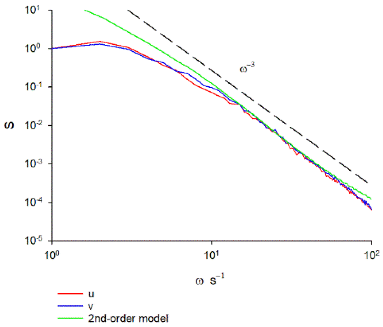
Experimental support for this prediction hinges on the fact that the velocity spectra for swarming insects is compatible with predictions from second-order models. Free roaming trajectories are predicted by first- and second-order models to be characterized by velocity spectra that decrease respectively as ω 2 and as ω 4   at high frequencies, whereas spectra decreasing faster than ω 4   can only be captured by third- or higher-order models [19,20]. Confinement within a swarm does not change these scaling behaviours (Appendix A). Instead, the quantity σ u σ x determines the position of the peak in the velocity spectra. The velocity spectra characterizing the trajectories of swarming non-biting midge Chironomus riparius recorded in quiescent conditions in the laboratory decreases approximately as ω 3 at the highest frequencies accessible (Figure 1). This scaling cannot arise in first order models but as illustrated, does arise at low frequencies in second order models when R ~ O ( 100 ) . This scaling is obtained for 19 different containing on average 15 to 94 individuals. Third-order processes are not evident.

4. Discussion

Herein it was argued that the trajectories of swarming insects like the trajectories of tracer particles in turbulence are at most described by second order models in which the position, velocity and acceleration of an insect are collectively Markovian, since higher-order processes even if present are not significant. This strengthens previously identified correspondences between swarming insects and the Lagrangian properties of high Reynolds number turbulence [23]. Their acceleration statistics have similar conditionally dependencies on velocity. These conditional dependencies only become apparent for u > 2 σ u and their occurrences may be attributed to occasional energetic rotations. The small size of this Reynolds number, R ~ O ( 100 ) , may be consequence of the fact that the average strength of the jerks, Equation (7b), increases with increasing Reynolds number: Equation (7b) can be rewritten as J = R 1 / 2 T 2 + σ u 2 σ x 2 u . At sufficiently high Reynolds numbers, jerks, like snaps, may have the potential to destabilize flight dynamics thereby causing the swarm to disintegrate. Indeed, the smallness of the estimate for the Reynolds number may be indicative of the susceptibility to swarming midges are to the disruptive impact of jerks. The swarm may also disintegrate at sufficiently low Reynolds numbers following a disordered-order phase transition [12], if the confining potential, a collective emergent property of disordered swarms [1,2], cannot emerge in ordered swarms or it may lose its collective properties if individuals remain in the vicinity of the swarm marker (a visually prominent marker over which swarm form). If this line of reasoning is correct, then the Reynolds number may be the result of fine tuning, as are other emergent properties of swarming [Reynolds 2024]. Jerks may also be particularly disruptive in swarms that are not asymptotically large (Appendix B).

Funding

The work at Rothamsted forms part of the Smart Crop Protection (SCP) strategic programme (BBS/OS/CP/000001) funded through the Biotechnology and Biological Sciences Research Council’s Industrial Strategy Challenge Fund.

Data Availability Statement

Data sharing not applicable to this article as no datasets were generated during the study.

Conflicts of Interest

The author declares no conflicts of interest.

Appendix A

Power spectra for first- and second-order autoregressive models of swarming insects
Here I show that the power spectra predicted by first- and second-order autoregressive models of the trajectories of swarming insects decrease respectively as ω 2 and ω 4 at high frequencies. That is, I show that confinement within a swarm does not upset the scaling behaviours obtained by Sawford [19] for freely roaming trajectories.
First-order autoregressive models of swarming insects
Okubo [1] classic one-dimensional model for the positions, x , and velocities, u , of swarming insects is given by
d u = u T d t σ u 2 σ x 2 x d t + 2 σ u 2 T d W
d x = u d t
where T is a velocity correlation timescale, σ x 2 is the position variance, σ u 2 is the velocity variance and d W i ( t ) is an incremental Wiener process with correlation property d W t d W t + τ ¯ = δ τ d t .
Okubo [1] showed that according to this model the velocity autocorrelation function is given by
R τ = e t 2 τ c o s ω 1 τ 1 2 ω τ s i n ω 1 τ
where ω 1 = σ u 2 σ x 2 1 4 T 2 1 / 2 .
It follows that the velocity power spectra is given by
f ω = 0 R τ c o s ω τ d τ = ω 2 / T 1 4 T 2 + ω 1 ω 2 1 4 T 2 + ω 1 + ω 2
At sufficiently high frequencies f ω ω 2 .
Second-order autoregressive models of swarming insects
The simplest second-order one-dimensional model for the positions, x , velocities, u , and accelerations, A , of swarming insects is given by
d A = 1 T + 1 t 2 A + σ u 2 σ x 2 x d t σ A 2 σ u   2 + σ u 2 σ x   2 u d t + 2 σ A   2 1 T + 1 t 2   d W
d u = A d t
d x = u d t
where   σ A 2 = σ u 2 / T t 2 is the acceleration variance and t 2 is a timescale representative of the smallest scales of motion [25].
It follows that for this model the velocity autocorrelation is a solution of the equation,
d 3 R d t 3 + 1 T + 1 t 2 d 2 R d t 2 + σ A 2 σ u   2 + σ u 2 σ x   2   d R d t + 1 T + 1 t 2 σ u 2 σ x 2 R = 0
The simplest solutions are single exponentials     e ξ τ where the inverse timescales ξ are solutions of the equation,
ξ 3 1 T + 1 t 2 ξ 2 + σ A 2 σ u   2 + σ u 2 σ x   2 ξ 1 T + 1 t 2 σ u 2 σ x 2 = 0
Typically, one solution, ξ 1 , is real whilst the other two, ξ 2 ± i Ω , are a pair of complex conjugate pair. In this case the general solution to Equation (A5) therefore takes the form,
R τ = A   e ξ 1 τ + 1 A   e ξ 2 τ c o s Ω τ B s i n Ω τ
where A and B are weighting factors.
It follows that,
f ω = A ξ 1 ξ 1 2 + ω 2 + 1 2 1 A ξ 2 ξ 2 2 + Ω ω 2 + ξ 2 ξ 2 2 + Ω + ω 2 + B ξ 2 Ω ξ 2 2 + Ω ω 2 + ξ 2 + Ω ξ 2 2 + Ω + ω 2
At sufficiently high frequencies
f ω c 2 ω 2 + c 4 ω 4 + O ω 6
where c 2 = A ξ 1 + 1 A ξ 2 + 1 A B Ω and c 4 = A 1 A B 3 ξ 2 2 Ω 3
Because the complexity of the general analytic expressions for ξ in terms of the model parameters, T , t 2 , and σ u 2 / σ u 2 precludes their application, here I present illustrative examples.
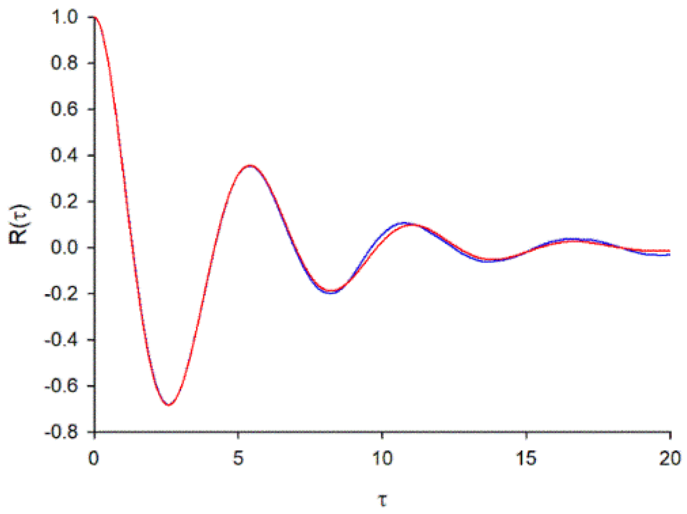
For T = t 2 = 1 , σ u 2 σ u 2 = 1 , ξ 1 1.54 , ξ 2,3 0.23 ± 1.12 i . The weighting factors A and B were found by minimizing the mean square difference between the predicted form of velocity autocorrelation, Equation (A7), and form obtained from simulation data obtained using Equation (A4) (Figure A1). This gave A = 0.24 and B = 0.065 . Consequently, c 2 0 and f ω ω 4 . The same scaling was obtained for T = t 2 = 1 , σ u 2 σ u 2 = 1 / 2 and for T = t 2 = 1 , σ u 2 σ u 2 = 2 .
Figure A1. Predicted form the velocity autocorrelation, Equation (A7), matches that obtained in numerical simulations. The trajectories of 10000 swarming insects were simulated by numerically integrating Equation (A4). Results are shown for T = t 2 = 1 , σ u 2 σ x 2 = 1 a.u.
Preprints 119832 g0a1

Appendix B

Jerks may destabilize small swarms
Reynolds [26] showed that the positions of the non-biting midge Chironomus riparius in laboratory swarms are maximally anticorrelated. In this case the average strength of the jerk experienced by the ith midge is given by
J i = σ A 2 σ u 2 δ i j + σ u 2 σ x 2 Λ i j u j
where Λ i j are elements of the inverse of the normalized position covariance matrix, the subscripts denote different individuals, and where there is summation of over repeated indices. The average strength of the jerk experienced by the ith midge therefore depends on the velocities of all individuals in the swarm, and so is unlikely to be aligned with the direction of travel (the major axis of the insect). If it were aligned, then the impact that jerks can have on flight dynamics would be minimized (see main text). This misalignment is, however, small in asymptotically large swarms which on average contain 10 or more individuals [5]. This is because u = 2 π σ u N 1 / 2 and because Λ i j = 1 when   i = j and Λ i j = 1 / N when   i j . Consequently,
J i = σ A 2 σ u 2 + σ u 2 σ x 2 u i σ u 3 σ x 2 O N 1 2
Despite their disruptive influence in small swarms, the maximal positional anticorrelations appear to dictate the approach to the asymptotic state (Appendix C).

Appendix C

Maximal anticorrelated positions and the asymptotic regime
Puckett and Ouellette [27] reported that once swarms contain order 10 individuals, all statistics saturate, and that the swarms enter an asymptotic regime. Puckett and Ouellette [27] also reported that the influence of the swarm marker (a visually prominent feature over which swarms nucleate) on the swarm morphology decays on a similar scale. Their results provide a strong constraint on how rapidly swarm models must produce collective states. Here I show that the observations of Puckett and Ouellette [27] together with the occurrence of maximal anticorrelated positions [26] are consistent with each individual in the swarm being on average located at a position that is mirror opposite to the average position of all other individuals, so that the average position of the ith individual in a swarm containing N individuals is given by x i = 1 N 1 j = 1 j i N x j . With this specification the least biased (maximum entropy) choice for the distribution of positions is the multivariant Gaussian
p x 1 , x 2 , x 3 , x N = 2 π σ c 2 N / 2 e x p 1 2 σ c 2 i = 1 N x i x i x i x i
where σ c 2 is a measure of the mean square size of the swarm. This can be rewritten as
p x 1 , x 2 , x 3 , x N = 2 π σ c 2 N / 2 e x p 1 2 σ c 2 x i Λ i j x j
where Λ i j = N N 1 if i = j and Λ i j = 3 N 4 N 1 2 if i j , and where there is summation of repeated subscripts. The distribution, Equation (A11), is realizable ( Λ i j   is positive definite) when N 3 .
Normalized positional covariances are, to good approximation, given by σ i j = 1 if
i = j and σ i j = 1 / N if i j , which is indicative of maximal anticorrelated positions.
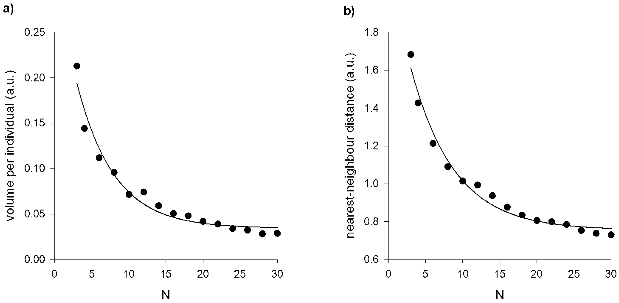
If the volume of the swarm, σ c 3 , is proportional to the population size, N, of the swarm then the volume per individual is predicted to saturate when swarms contain order 10 individuals, as observed by Puckett and Ouellette [27]. Puckett and Ouellette [27] found that the approach to the asymptotic state can be accurately represented by a decaying exponential function of the form V i n d = A e x p N N 0 + B where the characteristic scale N 0 = 3.1 ± 0.8 quantifies the rate of approach with increasing swarm size. Like the observations, model predictions are found to be accurately represented by the decaying exponential function albeit with N 0 1 .But in the presence of a swarm marker of size σ s = 1 (a.u.), the modelling predicts that N 0 5 (Figure A2). In such cases the distribution of positions becomes
p x 1 , x 2 , x 3 , x N = 2 π σ c σ s N e x p 1 2 σ c 2 x i Λ i j x j e x p 1 2 σ s 2 x i 2
Puckett and Ouellette [27] also reported on a related though distinct measure of how the midges arrange themselves in space, namely the average distance from an individual to its nearest neighbour. Puckett and Ouellette [27] found that like the volume per individual, the nearest-neighbour distance falls off rapidly with swarm size for small swarms, but eventually saturates. This behaviour is predicted by stochastic models of the 3-dimensional trajectories of swarming insects which by construction are exactly consistent with the multivariant distributions of positions, Equation (11). As observed [27] the characteristic scale, N 0 2 , is larger than for the volume per individual but is less than the observed characteristic scale, N 0 = 8.6 ± 2.0 . But in the presence of a swarm marker of size σ s = 1 (a.u.) the modelling predicts that N 0 6 (Figure A2).
Finally, the stochastic modelling predicts that the anticorrelation of spatial positions results in correlated accelerations, as evidenced in an analysis of pre-existing data (Figure A3). Such correlations have until now gone unnoticed, despite numerous attempts to uncover order in the dynamics of swarming insects [2,3,15,28,29].
This analysis leaves open the question as to how the velocity statistics approach the asymptotic regime.
Figure A2. a) Predicted volume per individual as a function of the number of individuals in the swarm. The solid line is an exponential fit, V i n d = A e x p N N 0 + B with N 0 5 . Puckett and Ouellette [27] reported that N 0 = 3.1 ± 0.8 . b) Predicted average distance from a given individual to its nearest neighbour as a function of the number of individuals in the swarm. The solid line is an exponential fit, d n n = A e x p N N 0 + B with N 0 6 . Puckett and Ouellette [27] reported that N 0 = 8.6 ± 2.0 .
Preprints 119832 g0a2
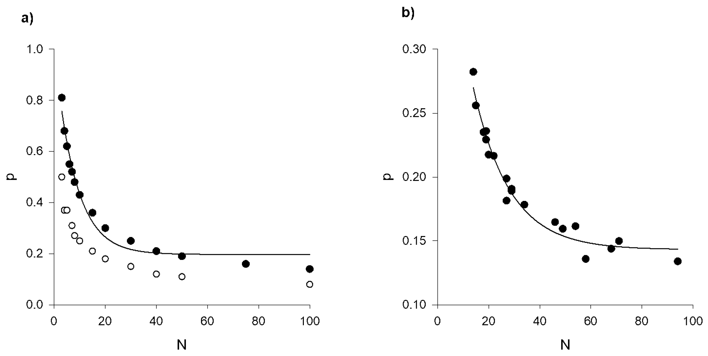
Figure A3. a) Predicted and b) observed net polarizations of acceleration as a function of the number individuals in the swarm (●). The polarization p = i = 1 N A i A i / N where A i is the acceleration of the ith individual and where the angular brackets denote a time average. Predictions were obtained using the stochastic model of Reynolds [26]. The experimental data is taken from Sinhuber et al. [24]. The solid lines are exponential fits, p = A e x p N N 0 + B with a) N 0 8 and b) N 0 14 . The average polarizations are significantly larger than the average polarizations that are predicted to arise sporadically in swarms of individuals with uncorrelated positions (o).
Preprints 119832 g0a3

References

  1. Okubo, A. Dynamical aspects of animal grouping: swarms, schools, flocks, and herds. Adv. Biophys. 1986, 22, 1–94. [Google Scholar] [CrossRef] [PubMed]
  2. Kelley, D.H. & Ouellette, N.T. Emergent dynamics of laboratory insect swarms. Sci. Rep. 2013, 3, 1073.
  3. Attanasi, A.; et al. Collective behaviour without collective order in wild swarms of midges. PLoS Comp. Biol. 2014, e1003697. [Google Scholar] [CrossRef]
  4. Attanasi, A.; et al. Finite-size scaling as a way to probe near-criticality in natural swarms. Phys. Rev. Lett. 2014, 113, 238102. [Google Scholar] [CrossRef]
  5. Puckett, J.G. and Ouellette, N.T. Determining asymptotically large population sizes of insect swarms. J. Roy. Soc. Int. 2014, 11, 20140710. [CrossRef]
  6. Sullivan, R.T. Insect swarming and mating. Florida Ent. 1981, 64, 44–65. [Google Scholar] [CrossRef]
  7. Cavagna, A.; et al. Characterization of lab-based swarms of Anopheles gambiae mosquitoes using 3D-video tracking. Sci. Rep. 2023, 13, 8745. [Google Scholar] [CrossRef]
  8. Reynolds, A.M., Sinhuber, M. & Ouellette N.T. Are midge swarms bound together by an effective velocity-dependent gravity? Euro. Phys. J. E 2017, 40, 46.
  9. Reynolds, A.M. Langevin dynamics encapsulate the microscopic and emergent macroscopic properties of midge swarms. J. Roy. Soc. Inter. 2018, 15, 20170806. [Google Scholar] [CrossRef]
  10. Reynolds, A.M. On the emergence of gravitational-like forces in insect swarms. J. Roy. Soc. Int. 2019, 16, 20190404. [Google Scholar] [CrossRef]
  11. Reynolds, A.M. Mosquito swarms shear harden. Eur. Phys. J. E. 2023, 46, 126. [Google Scholar] [CrossRef] [PubMed]
  12. Reynolds, A.M. Why insect swarms seem unduly complicated. Eur. Phys. J. Plus 2024, 139, 610. [Google Scholar] [CrossRef]
  13. Ni, R. & Ouellette, N.T. On the tensile strength of insect swarms. Phys. Biol. 2016, 13, 045002.
  14. van der Vaart, K., Sinhuber M., Reynolds, A.M., Ouellette, N.T. Mechanical spectroscopy of insect swarms. Sci. Adv. 2019, 5, eaaw9305.
  15. van der Vaart, K., Sinhuber, M., Reynolds, A.M. & Ouellette, N.T. Environmental perturbations induce correlations in midge swarms. J. Roy. Soc. Int. 2020, 17, 20200018.
  16. Reynolds, A.M. On the origin of the tensile strength of insect swarms. Phys. Biol. 2019, 16, 046002. [Google Scholar] [CrossRef]
  17. Reynolds, A.M. Understanding the thermodynamic properties of insect swarms. Sci. Rep. 2011, 11, 14979. [Google Scholar] [CrossRef]
  18. Sinhuber, M. van der Vaart, K., Feng, Y., Reynolds, A.M., Ouellette, N.T. An equation state for insect swarms. Sci. Rep. 2021, 11, 3773.
  19. Sawford, B.L. Reynolds number effects in Lagrangian stochastic models of turbulent dispersion. Phys. Fluids A 1991, 3, 1577–1586. [Google Scholar] [CrossRef]
  20. Reynolds, A.M. Third order Lagrangian stochastic modelling. Phys. Fluids 2003, 15, 2773–2777. [Google Scholar] [CrossRef]
  21. Reynolds, A.M., Yeo, K. & Lee, C. Anisotropy of acceleration in turbulent flows. Phys. Rev. E. 2004, 70, 017302.
  22. Viggiano, B.; et al. Modelling Lagrangian velocity and acceleration in turbulent flows as infinitely differentiable stochastic processes. J. Fluid Mech. 2020, 900, A27. [Google Scholar] [CrossRef]
  23. Reynolds, A.M. Insect swarms can be bound together by repulsive forces. Euro. Phys. J. E. 2020, 43, 39. [Google Scholar] [CrossRef] [PubMed]
  24. Sinhuber, M., van der Vaart, K., Ni, R., Puckett, J.G., Kelley, D.H. & Ouellette, N.T. Three-dimensional time-resolved trajectories from laboratory insect swarms. Sci. Data 2019, 6, 190036.
  25. Reynolds, A.M. & Ouellette, N.T. Swarm dynamics may give rise to Lévy flights. Sci. Rep. 2016, 6, 30515.
  26. Reynolds, A.M. Spatial correlations in laboratory insect swarms. J. Roy. Soc. Int. 2024 (In Press).
  27. Puckett, J.G. & Ouellette, N.T. Determining asymptotically large population sizes in insect swarms. J. Roy. Soc. Int. 2014, 11, 20140710.
  28. Ni, R. & Ouellette, N.T. Velocity correlations in laboratory insect swarms. Eur. Phys. J. Spec. Top. 2015, 224, 3271–3277.
  29. Puckett, J.G.; et al. Searching for effective forces in laboratory swarms. Sci. Rep. 2014, 4, 4766. [Google Scholar] [CrossRef]
Figure 1. Velocity spectra obtained by analysis of pre-existing data for laboratory swarms of the non-biting midge Chironomus riparius. Results are shown for the largest swarm in the dataset of Sinhuber et al. [24] which on average contains 94 individuals. Results are shown for the two horizontal components of velocity. The spectra are seen to decrease as ω 3 at the highest frequencies accessible in the experiment. Recordings were made at a rate of 100 Hz. The same scaling behaviour was obtained for smaller swarms. Shown for comparison is the velocity spectra predicted by a 2nd-order model with T = 1 ,     t 2 = 0.1 , σ x 2 = 1 and σ u 2 = 1 a.u. (Appendix A).
Preprints 119832 g001
Disclaimer/Publisher’s Note: The statements, opinions and data contained in all publications are solely those of the individual author(s) and contributor(s) and not of MDPI and/or the editor(s). MDPI and/or the editor(s) disclaim responsibility for any injury to people or property resulting from any ideas, methods, instructions or products referred to in the content.
Copyright: This open access article is published under a Creative Commons CC BY 4.0 license, which permit the free download, distribution, and reuse, provided that the author and preprint are cited in any reuse.
Prerpints.org logo

Preprints.org is a free preprint server supported by MDPI in Basel, Switzerland.

Subscribe

© 2024 MDPI (Basel, Switzerland) unless otherwise stated