Singular Value Decomposition (SVD) Method for LiDAR and Camera Sensor Fusion and Self-Calibration Algorithm

Preprint

Article

Singular Value Decomposition (SVD) Method for LiDAR and Camera Sensor Fusion and Self-Calibration Algorithm

Altmetrics

Downloads

Views

Comments

Kaiqiao Tian,

KaC Cheok,Micho Radovnikovich,Kazuyuki Kobayashi,

Changqing Cai^*

Kaiqiao Tian,

KaC Cheok,Micho Radovnikovich,Kazuyuki Kobayashi,

Changqing Cai^*

This version is not peer-reviewed

Submitted:

30 September 2024

Posted:

01 October 2024

You are already at the latest version

Alerts

Abstract

Lidar and camera sensors are widely utilized in autonomous vehicles (AVs) and robotics due to their complementary sensing capabilities—lidar provides accurate depth information, while cameras capture rich visual data. However, effective fusion of these sensors requires precise calibration, which is often challenging due to the differences in sensing modalities. This paper presents a self-calibration algorithm based on Singular Value Decomposition (SVD) to address this problem. Singular Value Decomposition is a powerful matrix factorization technique that helps identify key calibration parameters by decomposing matrices into singular vectors and values, representing essential calibration data. Our method not only automates the calibration process but also provides a reliable mechanism for detecting calibration errors, ensuring long-term accuracy and robustness in sensor fusion. The algorithm simplifies deployment in real-world applications by eliminating the need for manual calibration or external targets. Experimental results show that our approach improves sensor alignment and fusion accuracy, making it particularly useful for AV and robotic systems where maintaining precise calibration is critical.

Keywords:

Subject: Engineering - Electrical and Electronic Engineering

1. Introduction

Sensor fusion is a powerful technique that involves combining data from multiple sensors to obtain a more complete and accurate understanding of the environment. The integration of different types of sensors can provide complementary information, improving the overall quality and reliability of the data. One example of sensor fusion is the combination of data from LiDAR and camera sensors. LiDAR sensors use laser beams to detect the distance and position of objects in the environment, while camera sensors capture visual information that provides valuable context about the scene. LiDAR and camera fusion method enhances the safety and reliability of Advanced Driver Assistance Systems (ADAS) [1-4].

By merging LiDAR and camera data, it becomes possible to obtain a more comprehensive and precise understanding of the environment, which in turn enables better object detection and recognition. Several methods have been developed by scholars for data processing, such as fully convolutional neural networks method [5], Deep fusion method [6], data segmentation method [7-9]. These methods aim to improve the accuracy, efficiency, and robustness of data integration for applications such as autonomous driving and robotics. Advanced algorithms help in handling sensor data discrepancies, ensuring real-time synchronization, and enhancing object detection and perception capabilities. Before performing data fusion, the primary challenge is calibrating LiDAR and camera sensors. Calibration ensures that the data from both sensors can be accurately aligned and interpreted together. To calibrate the LiDAR Camera sensing system, we can use checkerboard for manual calibration [10-14] and increase calibration accuracy using mathematic method [15-18].

However, maintaining accurate calibration over time is a significant issue, as calibration can drift due to factors such as vibrations, temperature changes, and physical wear. Therefore, another major challenge is determining how to verify whether the calibration remains valid in the future and how to detect and correct any calibration errors that arise during long-term use. Addressing these challenges is critical for ensuring reliable sensor fusion and maintaining the overall performance of autonomous systems. Singular Value Decomposition (SVD) is a powerful mathematical tool widely used to address spatial rotation and transformation problems in various applications [19-21]. In this paper, we propose a novel method for self-calibration, self-correction, and error detection, leveraging the capabilities of SVD. Our approach allows for real-time adjustments to the calibration parameters of LiDAR and camera systems, ensuring accuracy over time. By systematically analyzing the calibration data, our method can identify and correct errors, thereby enhancing the reliability of multi-modal perception systems in advanced driver assistance applications.

2. Vehicle Platform Setup and Sensor Calibration

The calibration of LiDAR and Camera sensors is a crucial process that requires aligning their coordinate systems to facilitate precise data fusion. Due to their distinct measurement principles and units, it is necessary to transform their data into a standard coordinate system before fusing it. The calibration process usually involves collecting and preprocessing data, intrinsic and extrinsic calibration, and validation.

Calibrating LiDAR and Camera sensors can pose challenges due to their complexity and variability, and accurately modeling their internal parameters can be complex. Nonetheless, precise calibration is crucial for achieving accurate fusion of LiDAR and Camera data, which is vital for autonomous driving and other applications. Despite its importance, calibrating these sensors can be time-consuming and resource intensive. This chapter introduces a self-calibrating algorithm for LiDAR and Camera sensors to tackle these challenges. Automating the calibration process with this algorithm can significantly reduce the time and effort required for calibration while enhancing accuracy and consistency.

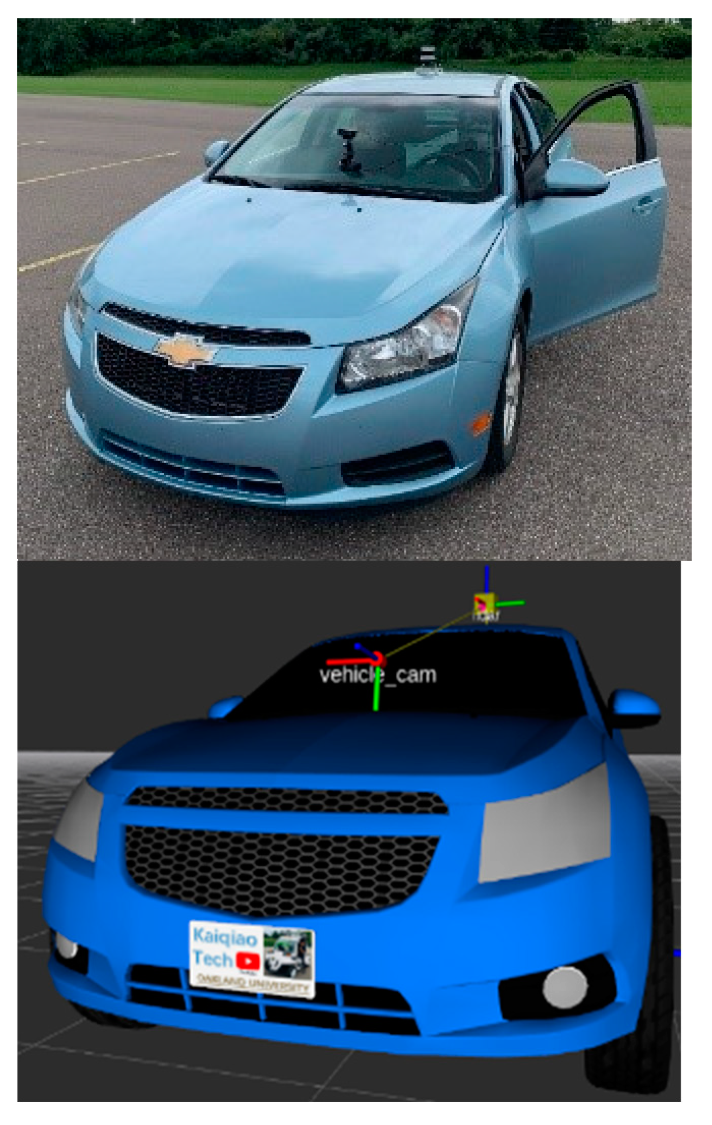
The algorithm development platform features a Chevrolet Cruse equipped with an Ouster 64 LiDAR mounted on the roof and a Logitech Camera attached to the windshield, as shown in Figure 1. The team designed a vehicle simulation model in ROS with identical dimensions and sensor placement to match the vehicle's length, height, and sensor position.

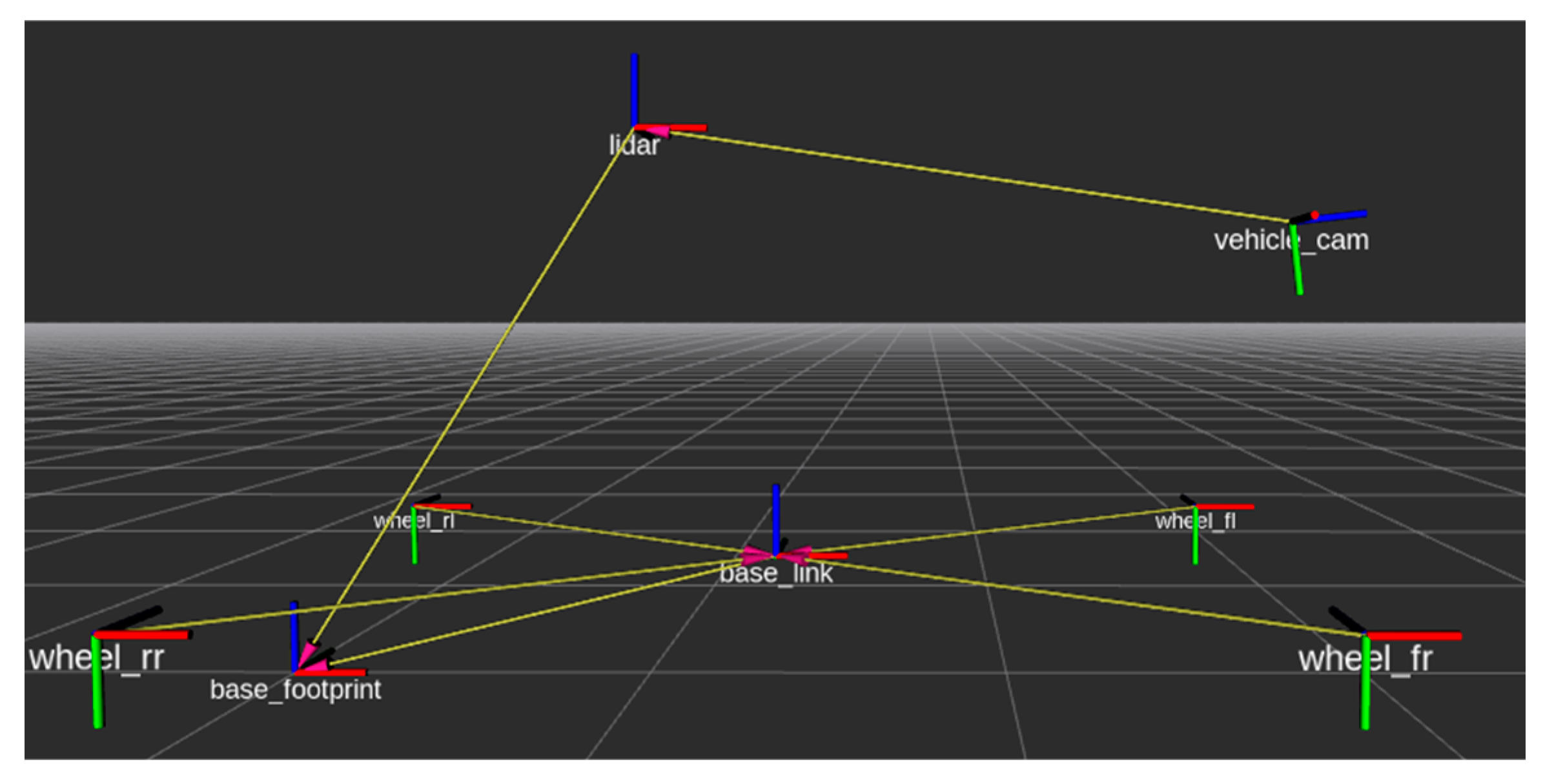
As shown in Figure 2, the TF tree for the vehicle model illustrates the spatial relationship between the vehicle body and its sensors in terms of Roll, Pitch, Yaw, x, y, and z values. The base_footprint frame represents the vehicle's lowest point on the ground, positioned at the midpoint between the rear wheels. The vehicle_cam frame displays the position of the camera in space and is also considered a child frame under the LiDAR frame

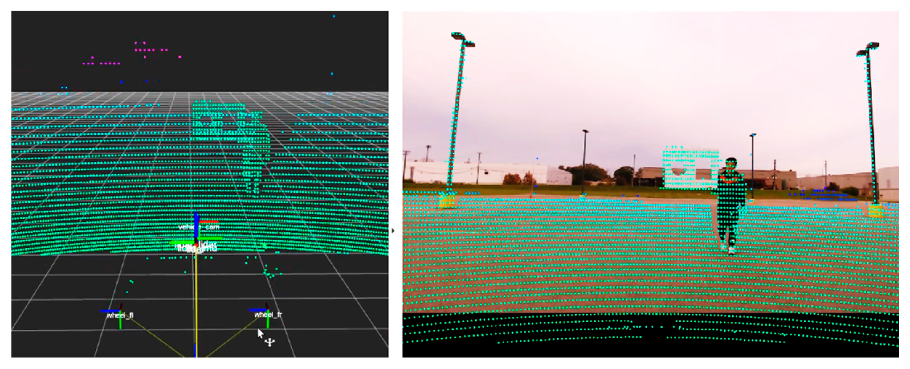
The accuracy of the sensor frames' transformation can significantly impact sensor fusion results. As depicted in Figure 3, LiDAR and Camera data fusion were tested using a checkerboard with two holes. In ROS RViz, the LiDAR point cloud data and vehicle TF tree are displayed, and all LiDAR points are aligned with the 2D image. The point cloud data presents the ground, tall lights, and the calibration board.

3. LiDAR and Camera Data Projection

To begin the LiDAR-to-2D image project, the first step involves determining the intrinsic and extrinsic parameters of the LiDAR and Camera sensors. The Camera's intrinsic parameters include the focal length, principal point, and distortion coefficients. In contrast, the extrinsic parameters describe the relative orientation and position of the LiDAR and Camera coordinate systems. With these parameters known, the 3D point cloud obtained from the LiDAR sensor can be transformed into the Camera coordinate system using the extrinsic parameters.

Transforming the 3D point cloud into the Camera coordinate system involves a rigid transformation that considers the position and orientation of the Camera relative to the LiDAR. This transformation enables the LiDAR data to be projected onto the 2D image plane of the Camera, which facilitates the creation of a 2D image that corresponds to the 3D point cloud. The accuracy of this transformation is crucial for ensuring that the resulting 2D image accurately represents the features and geometry of the 3D point cloud. PCD contains space points (x, y, z), and 2D images are presented by 2D pixels (x, y). The project 2D LiDAR can be obtained from the Camera intrinsic matrix and multiple extrinsic matrix.

P = K \times [R| t] = (\begin{matrix} 1 & 0 & x_{0} \\ 0 & 1 & y_{0} \\ 0 & 0 & 1 \end{matrix}) \times (\begin{matrix} f_{x} & 0 & 0 \\ 0 & f_{y} & 0 \\ 0 & 0 & 1 \end{matrix}) \times (\begin{matrix} 1 & \frac{s}{f_{x}} & 0 \\ 0 & 1 & 0 \\ 0 & 0 & 1 \end{matrix}) \times (I | t) \times (\begin{matrix} R & 0 \\ 0 & 1 \end{matrix})

(1)

The 2D rotation matrix for shown as below:

R_{x} = [\begin{matrix} 1 & 0 & 0 \\ 0 & c o s ϕ_{x} & - s i n ϕ_{x} \\ 0 & s i n ϕ_{x} & c o s ϕ_{x} \end{matrix}] R_{y} = [\begin{matrix} c o s Θ_{y} & 0 & s i n Θ_{y} \\ 0 & 1 & 0 \\ - s i n Θ_{y} & 0 & c o s Θ_{y} \end{matrix}] R_{z} = [\begin{matrix} c o s Θ_{z} & - s i n Θ_{z} & 0 \\ s i n Θ_{z} & c o s Θ_{z} & 0 \\ 0 & 0 & 1 \end{matrix}] J o i n t R o t a t i o n : R = R_{z} \cdot R_{y} \cdot R_{x}

(2)

Joint Rotation

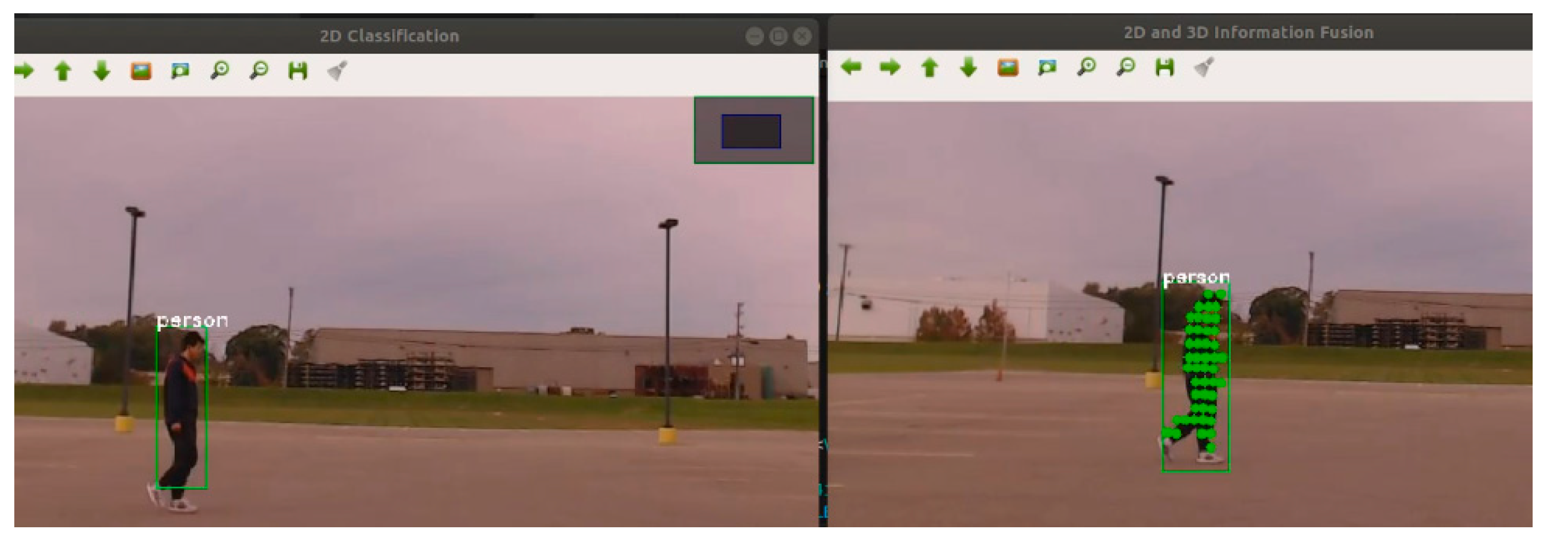
Figure 4 displays the outcome of the 2D projection of the PCD and the CNN classification. The YOLO neural network generated a green bounding box with a "person" label for the detected individual. A green dot on the image represents the 3D point cloud projected onto the 2D plane.

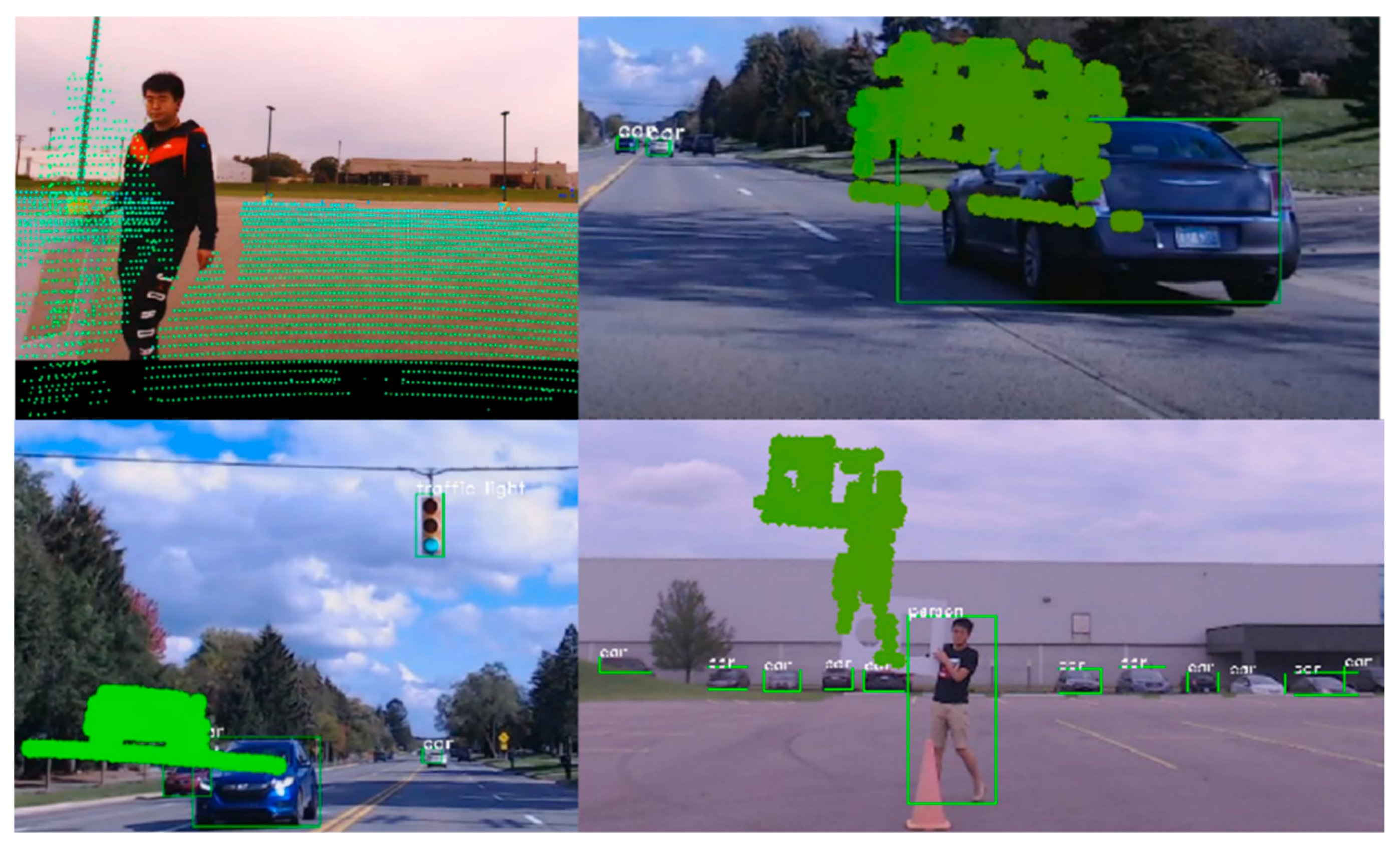
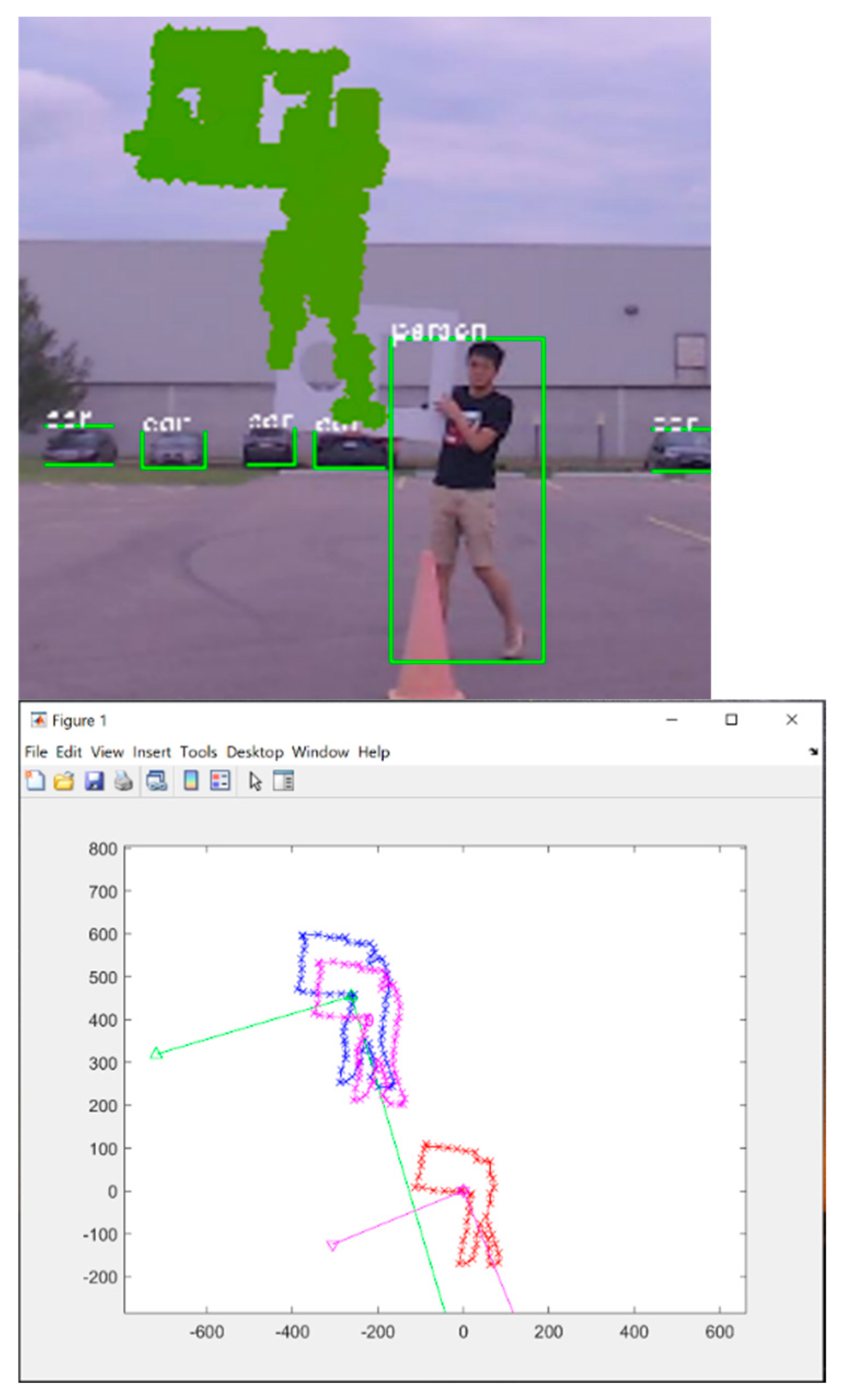
However, the main challenge in calibrating the Camera and LiDAR sensors for fusion is accurately determining the relative position and orientation of the two sensors. This requires defining the intrinsic parameters of each sensor (such as focal length, principal point, and distortion coefficients for cameras) and the extrinsic parameters that describe their relative positions and orientations. Calibration errors can lead to misalignment between the two-sensor data, resulting in inaccurate fusion and potentially compromising the output quality. Additionally, sensor hardware and mounting configuration differences can introduce additional challenges, requiring careful consideration during the calibration process. Figure 5 shows the LiDAR and Camera mis-calibration example in real data.

Another challenge in calibration is the time and effort required to collect and label data for calibration. This is particularly challenging for dynamic environments, where the scene constantly changes, and calibration data may need to be updated frequently to maintain accuracy.

Therefore, self-calibration algorithms are essential for LiDAR and camera sensor fusion because they help overcome the challenges and limitations of manual calibration methods.

4. Singular Value Decomposition Calibration Algorithm

Manual calibration of LiDAR and camera sensors can be time-consuming and lead to significant output discrepancies due to minor calibration errors. To address these challenges, a self-tuning algorithm can refine the calibration and automatically correct any mistakes in the transfer matrix. The initial step in this process involves identifying the 2D shapes of objects in both the camera and LiDAR data. To accomplish this, a contour hull creates an outline of the contour by tracing lines around the entire image, while a convex hull creates a convex curve around the object. The main difference between a contour and a convex hull is that a contour represents the boundary of an object, while a convex hull represents the minor convex shape that can contain a set of points. Contours can be irregular and have concave sections, while a convex hull is always a convex shape with straight edges connecting the points.

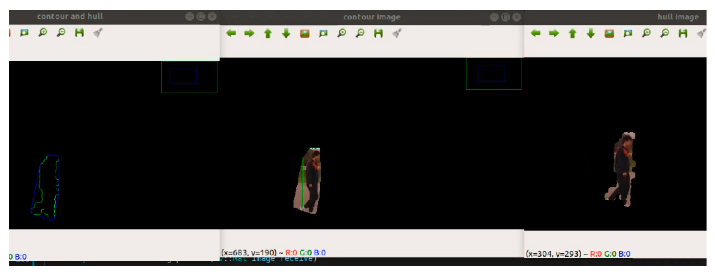
As shown in Figure 6, the blue line in the picture represents the 2D image contour, while the green line represents the convex hull.

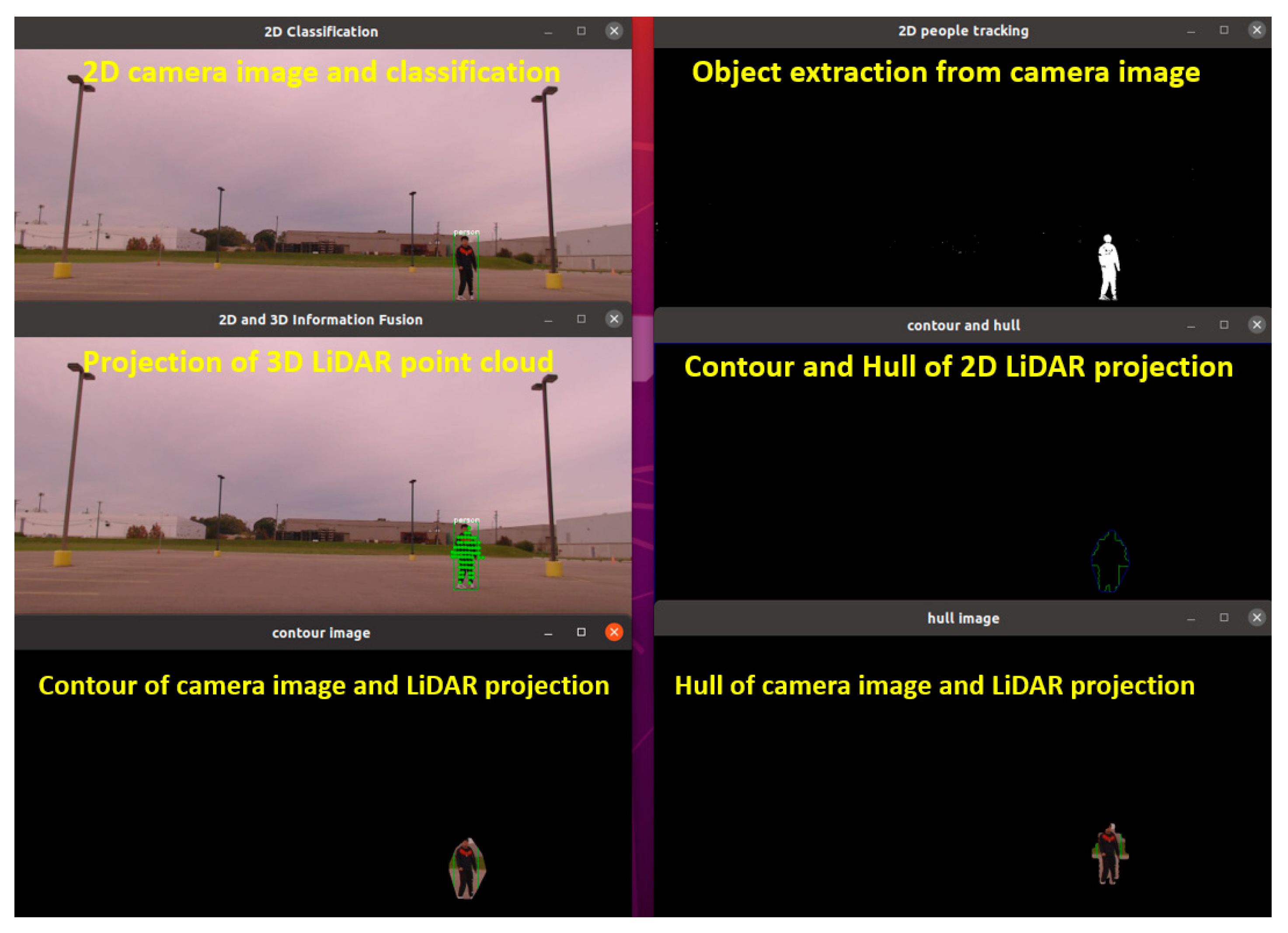
In LiDAR and camera fusion, 2D images track individuals' locations and create contours and convex hulls. Similarly, a 2D point cloud generates an alternative representation of individuals. An algorithm is then employed to compare these shapes in scale and rotation, resulting in an accurate transfer matrix. Figure 7 showcases all the preparatory data. The top left image depicts a 2D classification with people labeled in green. The top right image illustrates object tracking with a binary image decomposed into 2D pixel points. The middle-left picture shows LiDAR points projected onto the RGB image with green dots. The middle right picture shows the hull and contour algorithm that describes the tracked object. Finally, the bottom pictures exhibit the RGB image extracted by the contour and hull algorithms.

In the context of LiDAR and the Camera calibration algorithm, Singular Value Decomposition (SVD) is a powerful mathematical technique that can identify the relationship between LiDAR coordinates and camera coordinates by decomposing a matrix into three separate matrices. This helps uncover any patterns or features in the data and can be a valuable tool for understanding how the LiDAR and camera data relate to each other and optimizing the fusion algorithm. Additionally, the Gradient Descent (GD) algorithm can be used to optimize the SVD algorithm by minimizing the cost function of the machine learning model. By breaking the sensor fusion process into smaller, smoother steps, GD can help identify the distance vector and rotation matrix between LiDAR coordinates and Camera coordinates more efficiently, ultimately improving the accuracy and speed of the sensor fusion process. The LiDAR and camera calibration algorithm is a mathematical process that helps to align and synchronize the data from both sensors. This algorithm is developed and implemented using MATLAB software.

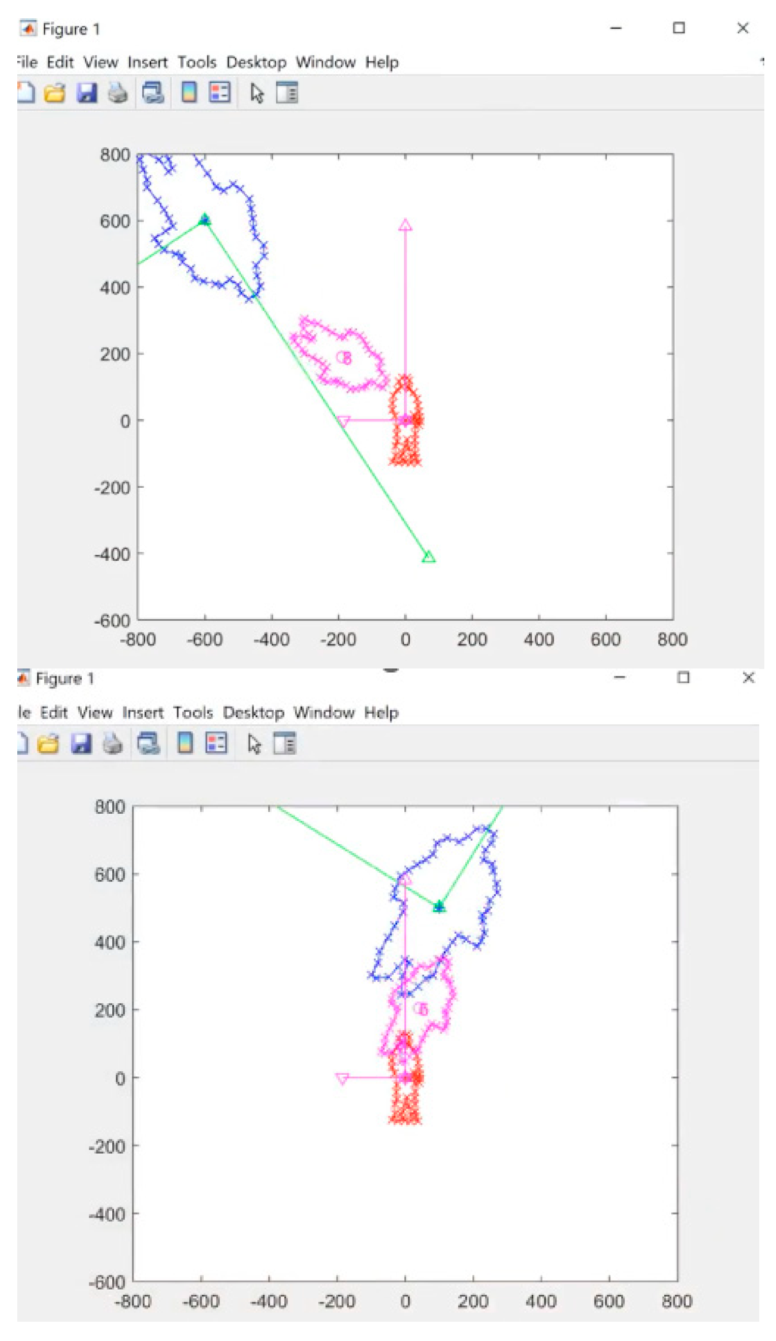
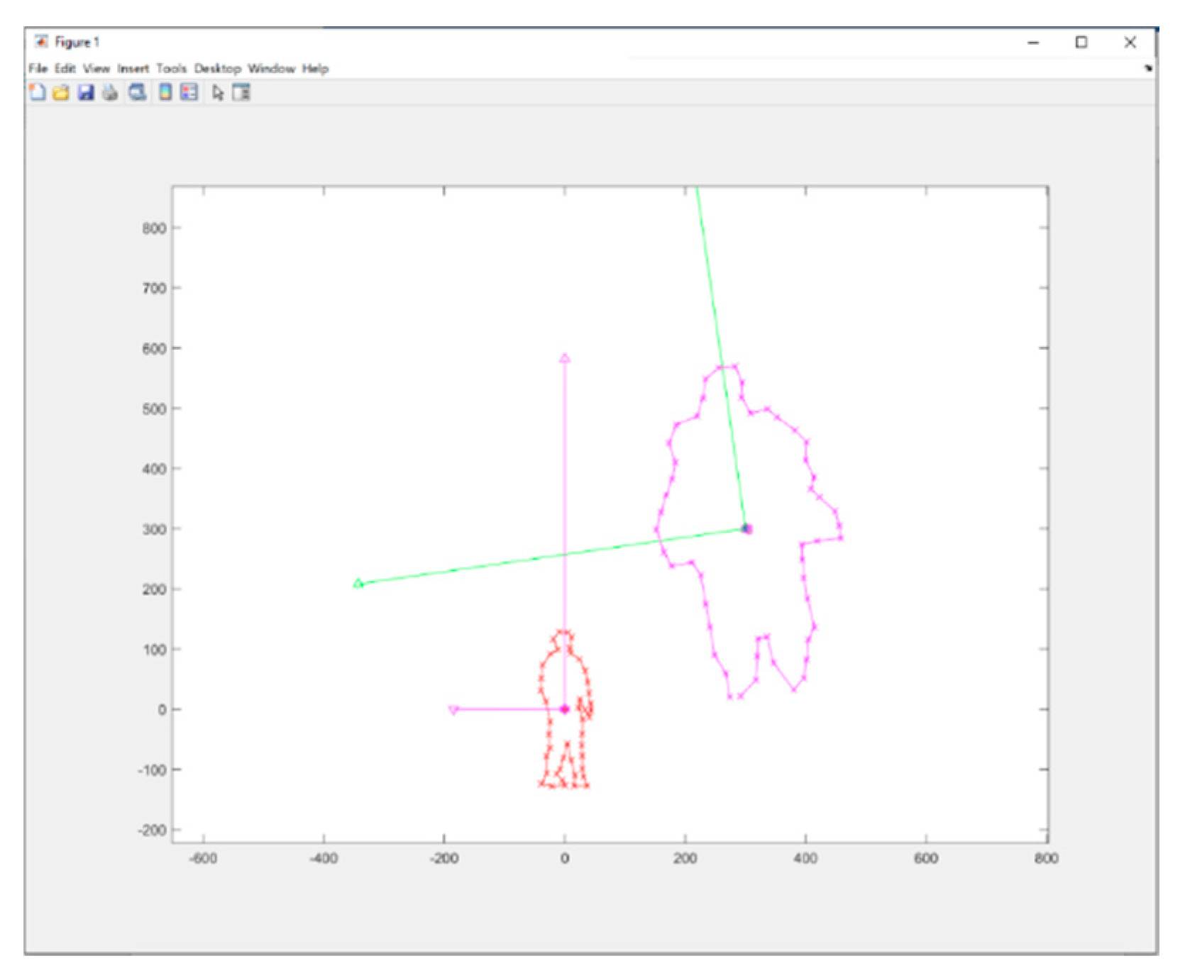
In the beginning, the algorithm takes the raw data from both LiDAR and camera sensors at time, which is shown in Figure 8. The red outline data represents the people detected by the camera in 2D, while the pink outline data represents the people detected by LiDAR. However, due to some random errors or misalignments, there might be a discrepancy between the two data sets, leading to a mis-calibration situation. This discrepancy can be in the form of incorrect scaling or rotation values.

The LiDAR and camera calibration algorithm is designed to identify and correct these random values, which will make the two systems well-matched and calibrated. By applying this algorithm, the discrepancies between the two data sets can be minimized, leading to more accurate and precise sensor fusion results.

Let’s denote and respective LiDAR data as matrix

p_{i}

and Camera data as matrix

q_{i}

p_{i} = {[\begin{matrix} p_{x} \\ p_{y} \\ p_{z} \end{matrix}]}_{i} = [\begin{matrix} p_{x_{i}} \\ p_{y_{i}} \\ p_{z_{i}} \end{matrix}] q_{i} = {[\begin{matrix} q_{x} \\ q_{y} \\ q_{z} \end{matrix}]}_{i} = [\begin{matrix} q_{x_{i}} \\ q_{y_{i}} \\ q_{z_{i}} \end{matrix}]

(1)

With reference to the p-frame, the distance vector and rotation matrix from the p-frame to the q-frame is:

d_{q}^{p} = {[\begin{matrix} x \\ y \\ z \end{matrix}]}_{q}^{p} R_{q}^{p} = [\begin{matrix} c o s ψ & - s i n ψ & 0 \\ s i n ψ & c o s ψ & 0 \\ 0 & 0 & 1 \end{matrix}] [\begin{matrix} c o s θ & 0 & s i n θ \\ 0 & 1 & 0 \\ - s i n θ & 0 & c o s θ \end{matrix}] [\begin{matrix} 1 & 0 & 0 \\ 0 & c o s ϕ & - s i n ϕ \\ 0 & s i n ϕ & c o s ϕ \end{matrix}] = [\begin{matrix} c ψ c θ & - s ψ c θ + c ψ s θ s ϕ & s ψ s ϕ + c ψ s θ c ϕ \\ s ψ c θ & c ψ c ϕ + s ψ s θ s ϕ & - c ψ s ϕ + s ψ s θ c ϕ \\ - s θ & c θ s ϕ & c θ c ϕ \end{matrix}]

(1)

The forward kinematics relationship between the position vector

p

and

q

is given by

p_{i} = d_{q}^{p} + R_{q}^{p} q_{i}

(1)

If a collection of m sets of data at each frame can be stored as matrix

P = [p_{1} p_{2} \dots p_{m}] Q = [q_{1} q_{2} \dots q_{m}]

(1)

Then, the following matrix relationship follow:

P = D_{q}^{p} + R_{q}^{p} Q D_{q}^{p} = d_{q}^{p} 1_{1 * m}

(1)

The relationship between the means of the data is similarly related as

\bar{p} = d_{q}^{p} + R_{q}^{p} \bar{p} w h e r e, \bar{p} = \frac{1}{m} \sum_{i = 1}^{m} p_{i}, \bar{q} = \frac{1}{m} \sum_{i = 1}^{m} q_{i}

(1)

Let

H

be the product

H = [P - \bar{P}] {[Q - \bar{Q}]}^{'}

, where

[P - \bar{P}]

be the variations of positions

P

from the mean position

\bar{p}

, where

\bar{P} = \bar{p} 1_{1 * m}

, and

{[Q - \bar{Q}]}^{'}

where

\bar{Q} = \bar{q} 1_{1 * m}

. The goal is decomposing

H = U S V^{'}

, where U and V are unitary matrices in the minimal singular value decomposition and S is a matrix of singular values of

H

Use the forward kinematics to express

H

as:

H = [D_{q}^{p} + R_{q}^{p} Q - D_{q}^{p} + R_{q}^{p} \bar{Q}] {[Q - \bar{Q}]}^{'} = R_{q}^{p} [Q - \bar{Q}] {[Q - \bar{Q}]}^{'}

(1)

Use similarity transformation for symmetric matrix to decompose relationship into:

H = R_{q}^{p} T_{Q Q} Λ_{Q Q} T_{Q Q}^{'} Λ_{Q Q} = [d i a g \{λ_{j} ([Q - \bar{Q}] {[Q - \bar{Q}]}^{'}), j = 1,2, 3; λ_{1} \geq λ_{2} \geq λ_{3}\}] λ_{j} = e i g e n v a l u e o f [Q - \bar{Q}] {[Q - \bar{Q}]}^{'} T_{Q Q} = m o d a l m a t r i x o f [Q - \bar{Q}] {[Q - \bar{Q}]}^{'} T_{Q Q}^{'} = T_{Q Q} o r T_{Q Q}^{'} = I

(1)

Decomposing

H

using SVD:

H = U S V^{'}

(1)

Where,

S = [d i a g \{\sqrt{λ_{j} (H^{'} H)}, j = 1,2, 3; λ_{1} \geq λ_{2} \geq λ_{3}\}] U U^{'} = U^{'} U = I V^{'} V = {V V}^{'} = I

(1)

It is seen that,

H^{'} H = [Q - \bar{Q}] {[Q - \bar{Q}]}^{'} {R_{q}^{p}}^{'} R_{q}^{p} [Q - \bar{Q}] {[Q - \bar{Q}]}^{'} = {[[Q - \bar{Q}] {[Q - \bar{Q}]}^{'}]}^{2}

(1)

So, it turns out that,

S = [d i a g \{\sqrt{λ_{j} (H^{'} H)}, j = 1,2, 3\}] = [d i a g \{\sqrt{λ_{j} ({[[Q - \bar{Q}] {[Q - \bar{Q}]}^{'}]}^{2})}, j = 1,2, 3\}] = [d i a g \{λ_{j} ([Q - \bar{Q}] {[Q - \bar{Q}]}^{'}), j = 1,2, 3\}] = Λ_{Q Q}

(1)

From the relationship

H = R_{q}^{p} T_{Q Q} Λ_{Q Q} T_{Q Q}^{'} = U S V^{'}

, one finds that

H = R_{q}^{p} T_{Q Q} V^{'} = T_{Q Q}^{'}

(1)

Therefore, the rotation matrix between LiDAR and Camera can be present as:

R_{q}^{p} = U V^{'}

(1)

Once we have obtained the rotation matrix that describes the orientation between the LiDAR and Camera, we can input this result into the Gradient Descent function. This function allows us to iteratively optimize the values of rotation and the distance scale vector by minimizing the cost function. This helps us to obtain more accurate results. Once we have calculated the optimal values for these parameters, we can apply the new frame transfer tree to get a more precise estimate of the orientation and distance between the LiDAR and Camera.

The designed Gradient Descent state present as:

θ = [p_{x_{i}}, p_{y_{i}}, s, r a d M a j b]

(1)

Where,

p_{x_{i}}, p_{y_{i}}

are the LiDAR data (able switch to Camera data); s is the scale change between LiDAR and Camera data, initial as 1; radMajb is the major rotation calculated from SVD algorithm,

r a d M a j b = a t a n 2 (V^{'} (2,1) V^{'} (1,1))

Gradient Decent iteration process:

θ_n e w = θ_o l d - γ \nabla J (θ)

(1)

The derivative cost function present as:

\nabla J (θ) = [2 q_{1} (p_{x_{i}} - {\bar{p}}_{x_{i}}), 2 q_{2} (p_{y_{i}} - {\bar{p}}_{y_{i}}), - 2 q_{3} (r a d M a j a - s * r a d M a j a) * s, - 2 q_{4} (r a d M a j a - r a d M a j b)]

(1)

Where,

q = [q_{1}, q_{1}, q_{1}, q_{1}]

is an adjust matrix.

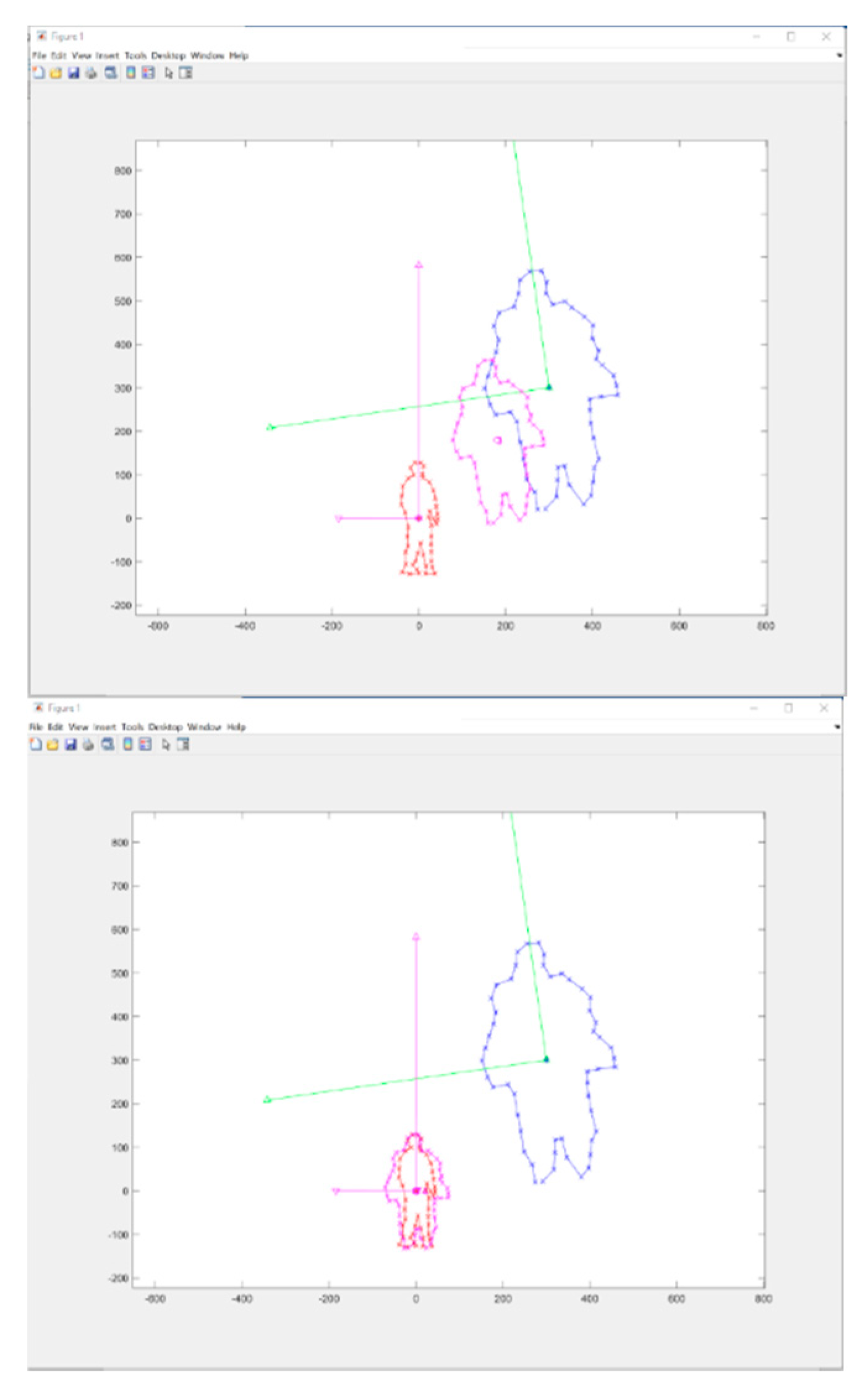
After deriving the necessary equation for the calibration process, MATLAB can be used to implement and execute the required computations. Figure 9 provides a visual representation of the LiDAR data changing as a result of rotation, scale, and position adjustments during the gradient descent iteration from

t_{0}

t_{n}

. As the calibration process iteratively optimizes these parameters, the LiDAR data eventually matches the target data with minimal error in rotation, scale, and position. This figure allows us to see the calibration process in action and visualize the changes to the LiDAR data as the calibration progresses.

The combination of the Singular Value Decomposition (SVD) and Gradient Descent (GD) algorithms provides a highly effective approach for completing the LiDAR and Camera calibration task. We can achieve fast and accurate results by tuning the parameters of both algorithms. Additionally, the designed algorithm is not limited to a specific type of sensor or calibration system, making it versatile and applicable in various contexts.

5. Results

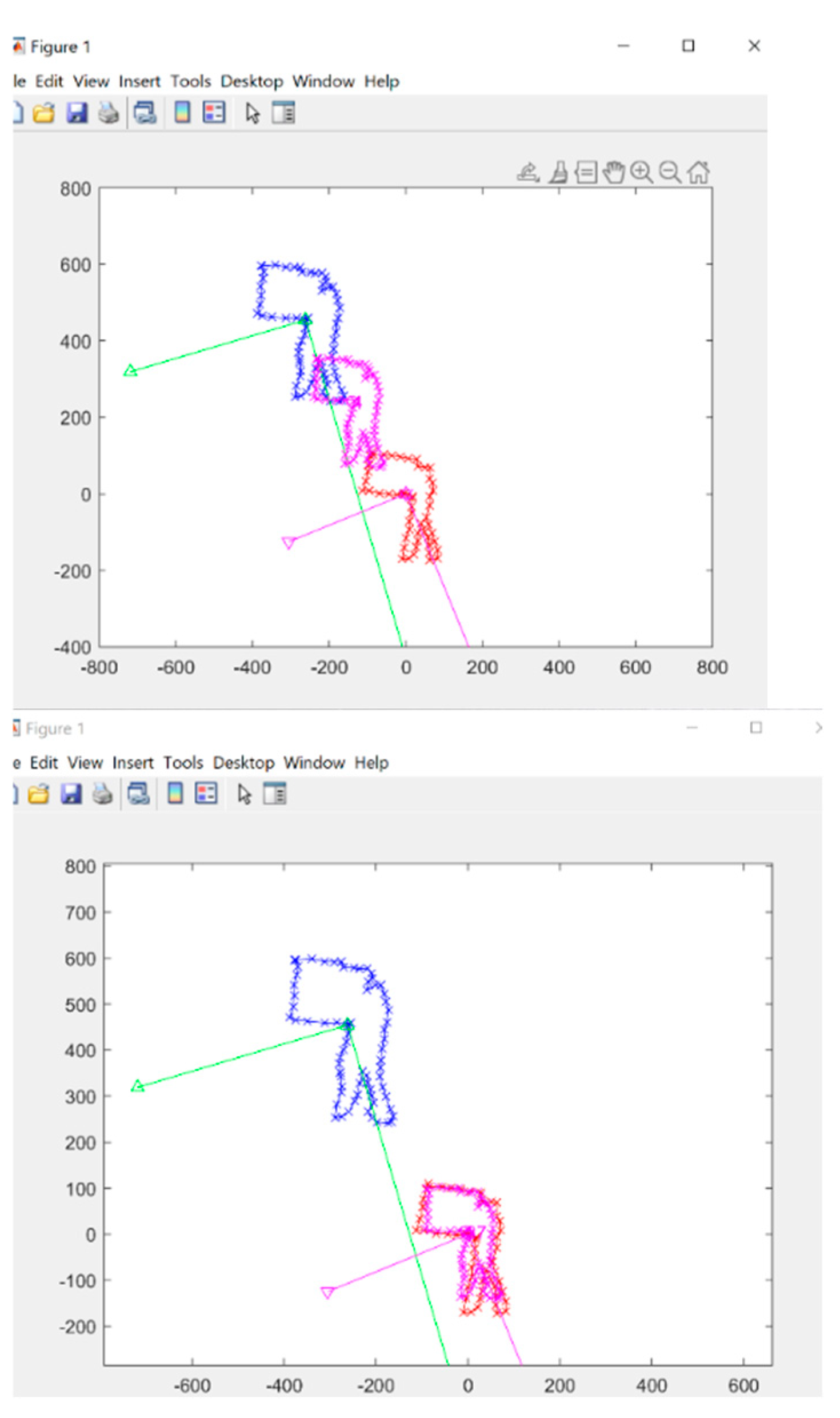
Figure 10 illustrates the mis-calibration of the LiDAR-Camera sensor fusion, and correction from

t_{0}

t_{n}

. The LiDAR data is represented by blue points, the Camera data by red points, and the processing state by pink points.

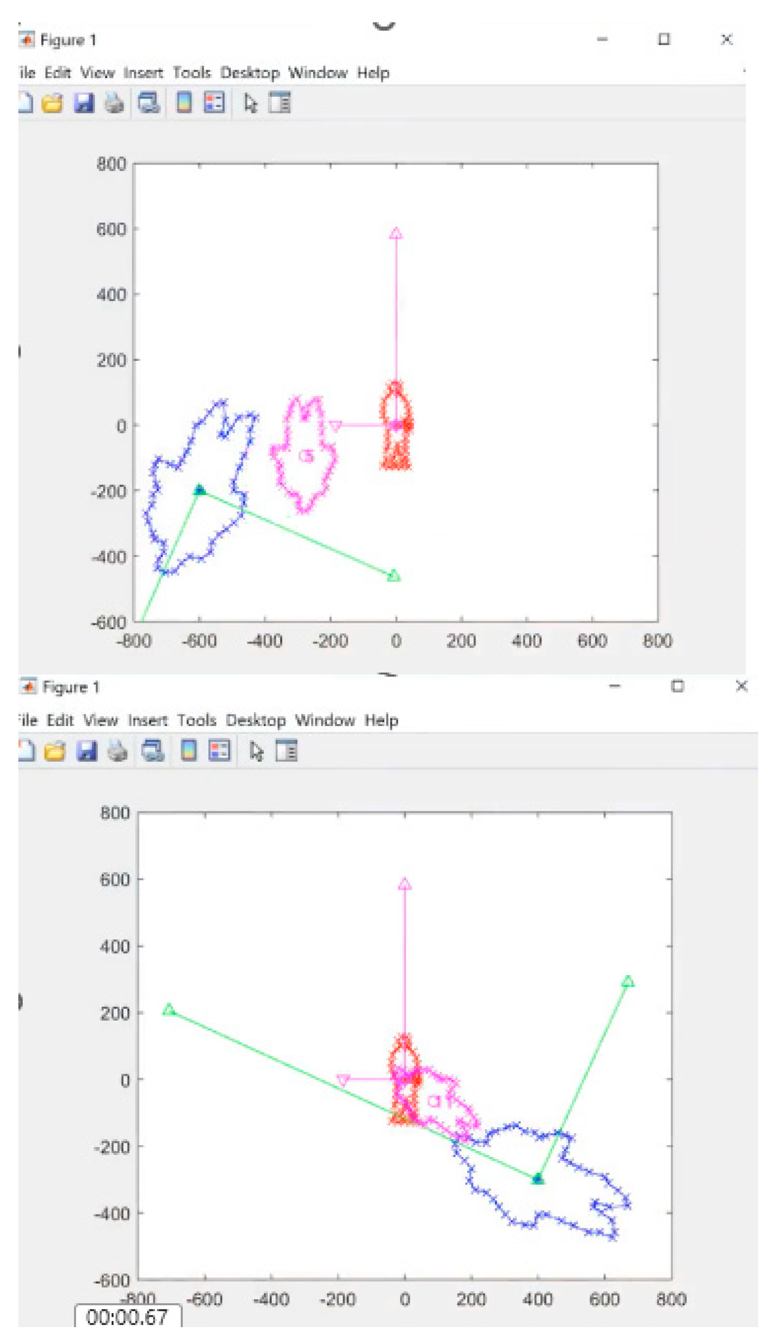
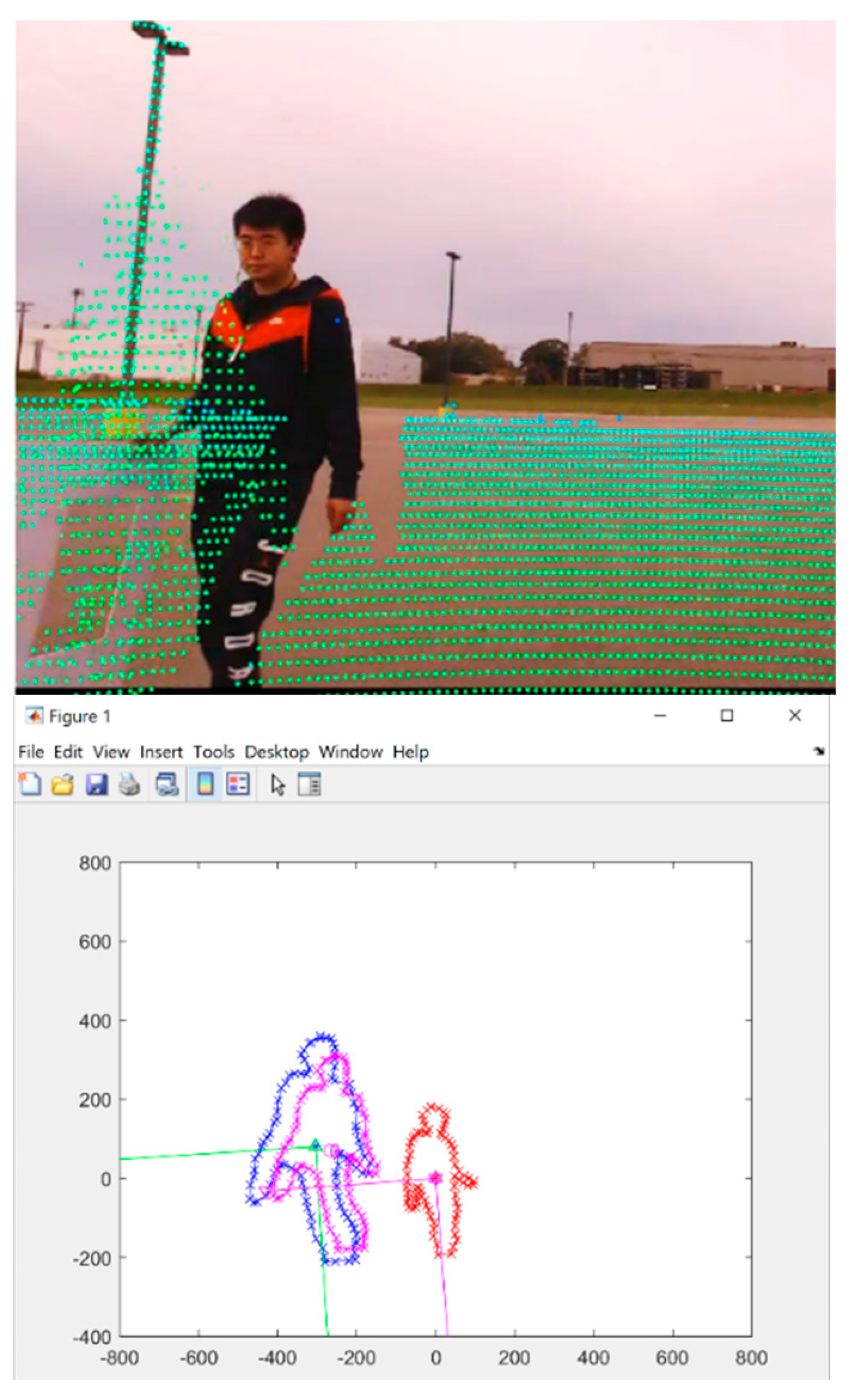
Figure 12 displays an example of mis-calibration where the LiDAR data exhibits scale change and offset in relation to the Camera data. This may be caused by errors in the Camera's TF tree or distortion calibration. On the other hand, this figure also illustrates how the self-calibration algorithm can effectively solve this issue.

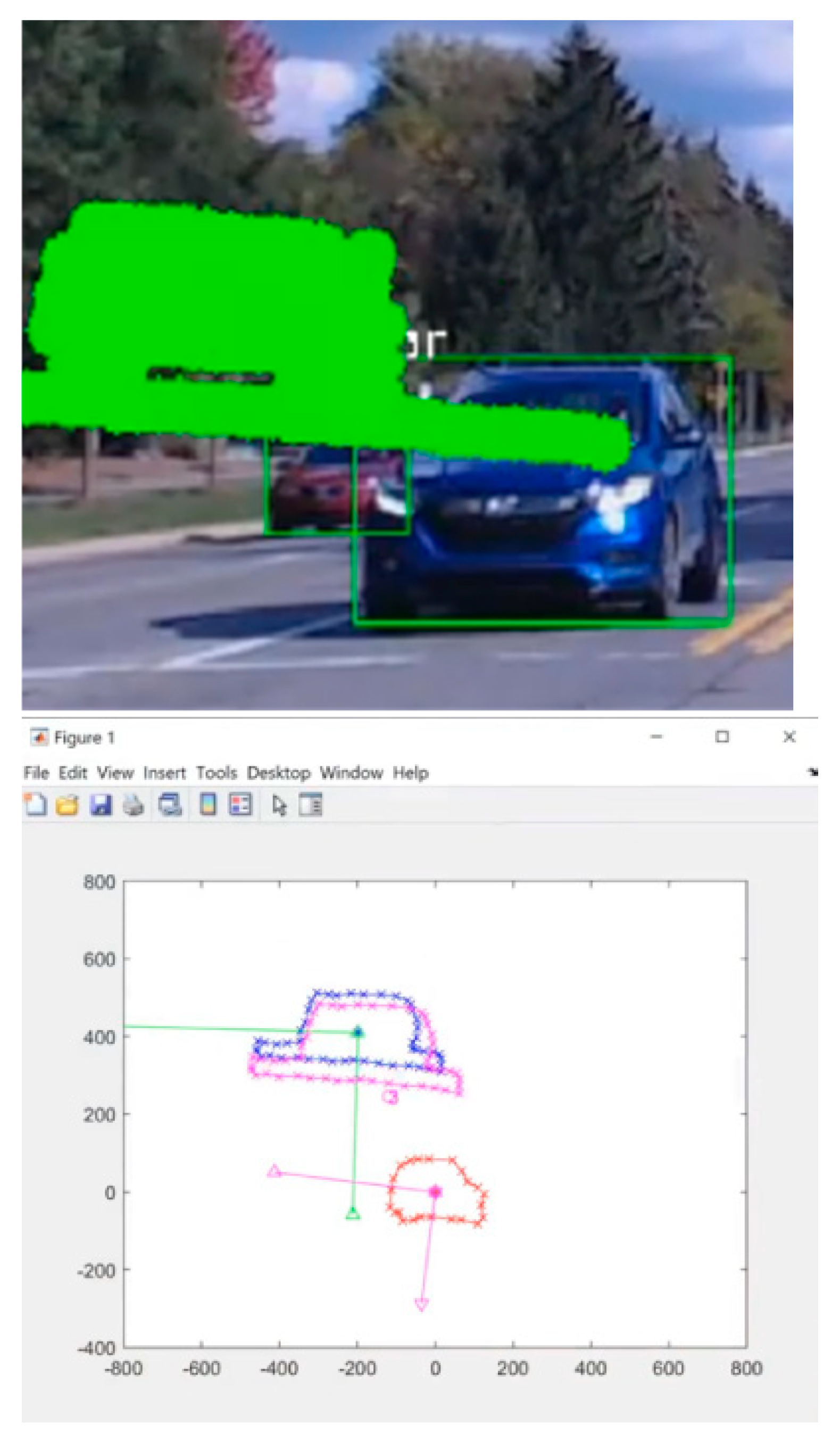
When self-driving vehicles operate on the highway, the position of their sensors may be affected by strong winds or vibrations. As illustrated in Figure 14, the LiDAR data appears to be positioned above the Camera detection. This figure also demonstrates the algorithmic processing involved in addressing this issue.

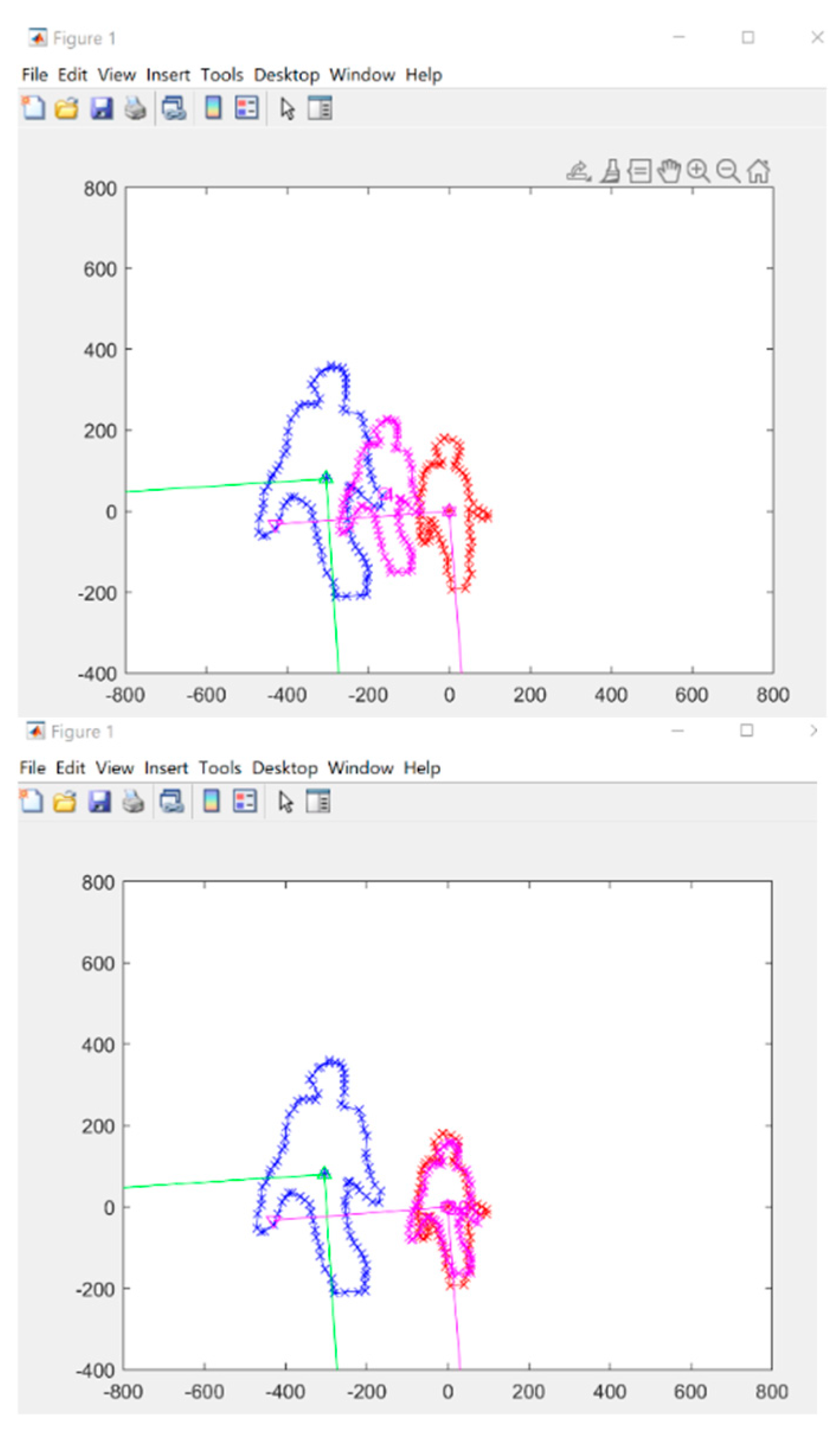
To test the limitations of the designed LiDAR and Camera self-calibration algorithm, we deliberately introduced manual offsets and rotations to the LiDAR data and subsequently applied the algorithm. The results are visually represented in Figure 18. Upon examining the outcomes, it is evident that the algorithm is capable of accurately identifying the correct transformation matrix from LiDAR to Camera, even in the presence of these intentional distortions

Figure 15. Self-calibration example 5 and 6 at time

t_{n / 2}

Figure 15. Self-calibration example 5 and 6 at time

t_{n / 2}

Figure 16. Self-calibration example 7 and 8 at time

t_{n / 2}

Figure 16. Self-calibration example 7 and 8 at time

t_{n / 2}

6. Conclusions

This paper addresses the implementation of a LiDAR-Camera perception system for standard home-use vehicles. It discusses the significant challenges involved in calibrating LiDAR and camera sensors, as potential miscalibration can lead to dangerous inaccuracies in object detection, which is critical for the safety and reliability of autonomous vehicles. The chapter introduces a robust self-calibration algorithm specifically designed for the LiDAR-Camera system. This algorithm leverages 2D image classification results obtained from Convolutional Neural Networks (CNN) alongside point cloud 2D projection data to ensure precise alignment of sensor data. The integration of CNNs enhances the system's ability to accurately classify and identify objects within the captured images, thereby improving the effectiveness of the calibration process.

Moreover, this algorithm incorporates self-calibration, self-correction, and error detection capabilities, collectively enhancing overall accuracy and robustness. The self-calibration process continuously adjusts the sensor parameters based on real-time data, while self-correction actively compensates for any detected discrepancies in sensor alignment. Error detection mechanisms further ensure that any potential inaccuracies are identified and addressed promptly, minimizing risks during operation. To determine the optimal transformation matrix for the sensors, the algorithm employs the Singular Value Decomposition (SVD) method in conjunction with gradient descent techniques. This powerful combination allows for effective integration of data from both LiDAR and camera sources, ensuring accurate sensor fusion and improving detection reliability across varying conditions.

Data Availability Statement

The data presented in this study are available on request from the corresponding author.

Acknowledgments

All authors would like to sincerely thank the reviewers and editors for their suggestions and opinions for improving this article.

Conflicts of Interest

The authors declare no conflicts of interest

References

Zhang, F. , D. and Knoll, A., 2014, October. Vehicle detection based on LiDAR and camera fusion. In 17th International IEEE Conference on Intelligent Transportation Systems (ITSC) (pp. 1620-1625). IEEE., 2nd ed.; 2007; Volume 3, pp. 154–196. [Google Scholar]
Caltagirone, L. , Bellone, M., Svensson, L. and Wahde, M., 2019. LIDAR–camera fusion for road detection using fully convolutional neural networks. Robotics and Autonomous Systems, 111, pp.125-131.Author 1, A.B.; Author 2, C. Title of Unpublished Work. Abbreviated Journal Name year, phrase indicating stage of publication (submitted; accepted; in press).
Zhao, X. , Sun, P., Xu, Z., Min, H. and Yu, H., 2020. Fusion of 3D LIDAR and camera data for object detection in autonomous vehicle applications. IEEE Sensors Journal, 20(9), pp.4901-4913.
Zhong, H., Wang, H., Wu, Z., Zhang, C., Zheng, Y. and Tang, T., 2021. A survey of LiDAR and camera fusion enhancement. Procedia Computer Science, 183, pp.579-588.Title of Site. Available online: URL (accessed on Day Month Year).
Caltagirone, L. , Bellone, M., Svensson, L. and Wahde, M., 2019. LIDAR–camera fusion for road detection using fully convolutional neural networks. Robotics and Autonomous Systems, 111, pp.125-131.
Li, Y.; Yu, A.W.; Meng, T.; Caine, B.; Ngiam, J.; Peng, D.; Shen, J.; Lu, Y.; Zhou, D.; Le, Q.V.; Yuille, A. Deepfusion: Lidar-camera deep fusion for multi-modal 3d object detection. In Proceedings of the IEEE/CVF conference on computer vision and pattern recognition; pp. 17182–17191.
Zhao, L. , Zhou, H., Zhu, X., Song, X., Li, H. and Tao, W., 2023. Lif-seg: Lidar and camera image fusion for 3d lidar semantic segmentation. IEEE Transactions on Multimedia, 26, pp.1158-1168.
Berrio, J.S. , Shan, M., Worrall, S. and Nebot, E., 2021. Camera-LIDAR integration: Probabilistic sensor fusion for semantic mapping. IEEE Transactions on Intelligent Transportation Systems, 23(7), pp.7637-7652.
Li, J. , Zhang, X., Li, J., Liu, Y. and Wang, J., 2020. Building and optimization of 3D semantic map based on Lidar and camera fusion. Neurocomputing, 409, pp.394-407.
Huang, J.K. and Grizzle, J.W., 2020. Improvements to target-based 3D LiDAR to camera calibration. IEEE Access, 8, pp.134101-134110.
Pusztai, Z. and Hajder, L., 2017. Accurate calibration of LiDAR-camera systems using ordinary boxes. In Proceedings of the IEEE international conference on computer vision workshops (pp. 394-402).
Veľas, M. , Španěl, M., Materna, Z. and Herout, A., 2014. Calibration of rgb camera with velodyne lidar.
Grammatikopoulos, L. , Papanagnou, A., Venianakis, A., Kalisperakis, I. and Stentoumis, C., 2022. An effective camera-to-LiDAR spatiotemporal calibration based on a simple calibration target. Sensors, 22(15), p.5576.
Tsai, D. , Worrall, S., Shan, M., Lohr, A. and Nebot, E., 2021, September. Optimising the selection of samples for robust lidar camera calibration. In 2021 IEEE International Intelligent Transportation Systems Conference (ITSC) (pp. 2631-2638). IEEE.
Li, X. , Xiao, Y., Wang, B., Ren, H., Zhang, Y. and Ji, J., 2023. Automatic targetless LiDAR–camera calibration: a survey. Artificial Intelligence Review, 56(9), pp.9949-9987.
Li, X. , Duan, Y., Wang, B., Ren, H., You, G., Sheng, Y., Ji, J. and Zhang, Y., 2024. Edgecalib: Multi-frame weighted edge features for automatic targetless lidar-camera calibration. IEEE Robotics and Automation Letters.
Tan, Z. , Zhang, X., Teng, S., Wang, L. and Gao, F., 2024. A Review of Deep Learning-Based LiDAR and Camera Extrinsic Calibration. Sensors, 24(12), p.3878.
Yamada, R. and Yaguchi, Y., 2024. Probability-Based LIDAR–Camera Calibration Considering Target Positions and Parameter Evaluation Using a Data Fusion Map. Sensors, 24(12), p.3981.
Bisgard, J. , 2020. Analysis and linear algebra: the singular value decomposition and applications (Vol. 94). American Mathematical Soc.
Jaradat, Y. , Masoud, M., Jannoud, I., Manasrah, A. and Alia, M., 2021, July. A tutorial on singular value decomposition with applications on image compression and dimensionality reduction. In 2021 international conference on information technology (ICIT) (pp. 769-772). IEEE.
He, Y.L. , Tian, Y., Xu, Y. and Zhu, Q.X., 2020. Novel soft sensor development using echo state network integrated with singular value decomposition: Application to complex chemical processes. Chemometrics and Intelligent Laboratory Systems, 200, p.103981.

Figure 1. Vehicle platform and ROS simulation.

Figure 2. Vehicle platform sensor system transfer frame tree.

Figure 3. LiDAR and Camera manual calibration.

Figure 4. Camera CNN detection and LiDAR PCD 2D projection.

Figure 5. Calibration error results in LiDAR and Camera sensor fusion.

Figure 6. 2D Image pedestrian tracking using contours and convex hull algorithms.

Figure 7. Combining 2D image and 3D point cloud data.

Figure 8. Camera and LiDAR contours calibration process at time

t_{0}

Figure 8. Camera and LiDAR contours calibration process at time

t_{0}

Figure 9. Camrea and LiDAR calibration process at time

t_{n / 2}

and

t_{n}

Figure 9. Camrea and LiDAR calibration process at time

t_{n / 2}

and

t_{n}

Figure 10. Schemes follow the same formatting.

Figure 11. Self-calibration example 1 at time

t_{n / 2}

and

t_{n}

Figure 11. Self-calibration example 1 at time

t_{n / 2}

and

t_{n}

Figure 12. Schemes follow the same formatting.

Figure 13. Self-calibration example 2 at time

t_{n / 2}

and

t_{n}

Figure 13. Self-calibration example 2 at time

t_{n / 2}

and

t_{n}

Figure 14. Self-calibration example 3 at time

t_{n / 2}

and

t_{n}

Figure 14. Self-calibration example 3 at time

t_{n / 2}

and

t_{n}

Disclaimer/Publisher’s Note: The statements, opinions and data contained in all publications are solely those of the individual author(s) and contributor(s) and not of MDPI and/or the editor(s). MDPI and/or the editor(s) disclaim responsibility for any injury to people or property resulting from any ideas, methods, instructions or products referred to in the content.

© 2024 by the authors. Licensee MDPI, Basel, Switzerland. This article is an open access article distributed under the terms and conditions of the Creative Commons Attribution (CC BY) license (http://creativecommons.org/licenses/by/4.0/).

Copyright: This open access article is published under a Creative Commons CC BY 4.0 license, which permit the free download, distribution, and reuse, provided that the author and preprint are cited in any reuse.

MDPI Initiatives

Important Links

Choose an area of interest and we will send you notifications of new preprints at your preferred frequency.

Disclaimer

Singular Value Decomposition (SVD) Method for LiDAR and Camera Sensor Fusion and Self-Calibration Algorithm

Abstract

1. Introduction

2. Vehicle Platform Setup and Sensor Calibration

3. LiDAR and Camera Data Projection

4. Singular Value Decomposition Calibration Algorithm

5. Results

6. Conclusions

Data Availability Statement

Acknowledgments

Conflicts of Interest

References

MDPI Initiatives

Important Links

Subscribe