
Submitted:
26 November 2024
Posted:
27 November 2024
You are already at the latest version
Abstract
Continuous and uncontrolled extraction of groundwater often creates tremendous pressure on groundwater levels. As a part of the sustainable planning and effective management of water resources, it is crucial to assess the existing as well as future groundwater level (GWL) condition. In the current study, an attempt was made to model and forecast GWL using artificial neural networks (ANN) and multivariate time series models. Autoregressive integrated moving average (ARIMA) and ARIMA incorporating exogenous variables (ARIMAX) were adopted as the time series models. Kushtia district in Bangladesh was selected as the case study area, and GWL data of five monitoring wells in the study are used to demonstrate the modeling exercise. Rainfall was taken as the exogeneous variable to explore whether its inclusion enhanced the performance of GWL forecasting using the developed models. The performance of each time series and ANN model was assessed based on various model evaluation criteria. It was evident from the results that the multivariate ARIMAX model (SSE of 15.361) performed better than the univariate ARIMA model with an SSE of 17.217 for GWL forecasting. This demonstrates the fact that the multivariate time series models generated enhanced forecasting of GWL compared to the univariate time series models. When comparing the time series and ANN models, it was found that the ANN-based model outperformed the time series models with the enhanced forecasting accuracy (SSE of 9.894). Results also exhibit a significant correlation coefficient value R of 0.995 (ANN 6-8-1) for the existing and predicted data. The current study conclusively proves the superiority of ANN over the time series models for the enhanced forecasting of GWL in the study area. Thus, the ANN approach was not only carried out for model building and simulation but also to provide a valuable tool for managing water resources amidst changing environmental conditions.
Keywords:
groundwater level
; exogenous variable
; ANN
; multivariate time series
; ARIMAX
1. Introduction
Bangladesh is one of the most densely populated countries in the world. There is population growth and increasing urbanization in addition to climate change. For this reason, stress on GW is increasing rapidly. This earthly resource is important, particularly for developing countries that support agricultural necessity and crop production, drinking purposes, and ecosystems. For this reason, accurate and reliable forecasting of GWL is necessary. Furthermore, it is also necessary for sustainable management of water resources and to facilitate the consumptive use of. Additionally, it plays a crucial role in the earth’s water cycle. Like many districts in Bangladesh, Kushtia relies heavily on agriculture, as a large irrigation project named the Ganges-Kobadak (G-K) Project that covers an area of 197,500 hectares serves the region. In this project, pumps are used to supply water from the river Ganges to the irrigation areas. According to the “Statistical Yearbook Bangladesh 2022” by the Bangladesh Bureau of Statistics (BBS), irrigation in Kushtia district is being carried out using different types of tube wells, including deep, shallow, and hand, as well as power pumps. The district’s approximately 68% area is covered by irrigation [1]. Forecasting of GW can help farmers optimize water use and improve crop yields. Besides that, the area experiences a substantial variation of rainfall (RF) (a rainfall pattern that can impact GW recharge rates); GWL prediction will help in planning for dry periods to minimize the severe impacts of droughts and floods. At times of drought, GW can play an important role when surface water is reduced by giving a buffer to help stabilize the water supply. The authors [2] analyzed the importance of safe water sources and assessed the conventional water sources, including GW.
GWLs in Bangladesh usually fluctuate on a seasonal basis due to the monsoon rains and dry periods, resulting in a significant impact on water availability all over the year. Urbanization as well as population growth are also matters of concern because the demand for GW is increasing due to these factors. GWL forecasting can help to manage this demand. Irrigation in this country heavily relies on GW due to sufficient surface water in the dry season, and future water demand will greatly depend on GW resources. GW is also affected by pollution; for instance, chemical fertilizers and pesticides used in fields contribute tremendously to its quality. Over-extraction of GW and the levels of the sea can lead to salinity intrusion problems in coastal areas in Bangladesh. Deforestation is a big problem in this country nowadays; it can change the recharge process of GW, which may decrease GW recharge. Studies from authors identified that RF is an important factor for the GW recharge potential [3]. Furthermore, RF is a significant influence on GW recharge potential [4]. Over-extraction of GW can be caused by inefficient irrigation practices because of the use of outdated or inadequate technology, which is widely recognized in the country; as a result, it can affect GW accessibility. The quality and availability of GW are decreasing gradually due to factors (man-made or natural) such as over-extraction, contamination (due to various reasons such as poor management of industrial or domestic wastewater), and climate change. The attenuation of GWLs is also a matter of concern.
The goals of this study are to model and predict GWLs using the ANN, the statistical time series autoregressive integrated moving average (ARIMA), and to incorporate an exogenous variable (RF) to analyze its effects. It is widely accepted that ANN- and ARIMA-based time series models (ARIMA, which is a univariate time series model and ARIMA incorporating exogenous variables (ARIMAX), which is essentially a multivariate time series model) are powerful tools for predicting various data. In recent times, time series analysis has gained significant popularity as a statistical method for creating forecast models, and its application has expanded worldwide [5]. GW is sometimes the only dependable supply of fresh water in many developing nations since it is widely accessible, relatively inexpensive to collect, and typically of higher quality than surface water [6,7]. This dependence on GW is especially noticeable in areas with little or highly contaminated surface water [8]. Over 70% of all irrigated land in Bangladesh is sustained by GW resources. The nation’s dense population, expanding agricultural needs, and quick industrialization are the main causes of this widespread reliance [9]. Lowering GWLs in agricultural areas might result in reduced crop yields because of limited water supplies, which exacerbates problems with food security [10,11]. Apart from the physical loss of GW, another major worry is its quality, especially in areas where contamination is common [12].
GWLs can be significantly impacted by the fluctuation of RF, which is a key source of GW recharge [13]. It is generally acknowledged that one of the most important ways to increase the precision of GWL predictions is to incorporate RF data into both ANN and ARIMA models [14]. Because of Bangladesh’s monsoon climate, the relationship between RF and GWL is especially significant there [15]. This study compares the ARIMA-based time series models and ANN models’ performances to determine which modeling strategy is best for forecasting GWL variations in the area. In summary, GW is an essential resource that needs to be managed carefully to maintain its sustainability. A crucial aspect of GW management is the prediction of GWL changes, which offer important insights into GW availability in the future and assist in formulating policies for its sustainable use [16,17].
GW is an almost worldwide source of superior freshwater [18]. The study is mainly focused on the modeling of GWLs using ANN- and ARIMA-based time series models and finding the best models based on their various performance evaluation criteria. Furthermore, a key focus of the research will be to find the future GWL conditions beyond the available well data to understand the upcoming situations in Kushtia, Bangladesh.
2. Study Area and Data Description
In the current study, Kushtia district, covering an area of 1608.8 km2 in the Khulna division of Bangladesh, is selected. Figure 1 shows the location of the study area, which is positioned in southwest Bangladesh. Encompassing the coordinates of 23°42′ to 24°12′ north and 88°42′ to 89°22′ east. Located in this area, the Ganges-Kobadak (G-K) irrigation project is an extensive surface irrigation network that serves the southwestern districts of Kushtia, Chuadanga, Magura, and Jhenaidah. The district has six upazilas, of which Daulatpur is the largest, totaling a population of 2,149,692 (according to the Population and Housing Census, 2022). For GWL modeling and prediction in the current study, five GW monitoring stations from each upazila (i.e., Bheramara, Daulatpur, Kushtia Sadar, Kumarkhali, and Mirpur) with an RF station are selected. The GWL data collected was on a weekly basis. Accordingly, data consisting of 414 weekly GWL readings from 1999 to 2006 were sourced from the Bangladesh Water Development Board (BWDB). The RF data obtained here is exogenous input and collected for the same periods. The GWL data available on a weekly basis has a unit of m.PWD, which is the public works datum (PWD) used by BWDB. The m.PWD is located at 0.46 m below the mean sea level (MSL).
The area is characterized by several rivers, such as the Ganges, Mathabhanga, Kaligonga, and Kumar, which flow across the district. Additionally, the district has a flat, alluvial landscape, which is typical for the delta region. The area is flat terrain and has fertile soil that makes it favorable to agriculture, which is highly dependent on irrigation. Moreover, Kushtia relies on GW as the main water source for irrigation, especially during the dry season when there is limited surface water availability. The area experiences an average maximum temperature of 37.8°C and an average minimum of 9.2°C. The yearly RF averages 1,467 millimeters.
The aquifers in the area consist of alluvial deposits, which include sand, silt, and clay. These are part of the Ganges-Brahmaputra Delta. These formations typically exhibit varying permeability that influences groundwater (GW) movement. Shallow aquifers are typically found at lesser depths and are mainly composed of alluvial deposits, and they are highly permeable. They are directly influenced by surface water and recharge primarily through RF and seasonal flooding. They are essential for local water supply, particularly for irrigation and domestic use. The deep aquifers may be recharged by lateral flow from surrounding areas. Recharge to the aquifers occurs through direct RF infiltration, irrigation return flows, and riverbank infiltration during the monsoon season. GW quality can vary, with some areas facing issues of salinity and arsenic contamination, which pose significant health risks. Authors found that the diffusivity (degrees of flow) varies from 181,143 m2/day to 256,788 m2/day, and the overall estimated parameter results of the aquifer system show that the area is hydrogeologically favorable for GW development provided the other conditions are fulfilled [19]. Information on the selected GWL monitoring stations and RF stations with locations are given in Table 1.
3. Methodology
The primary objective of this study is to model and forecast GWL changes using ANN and statistical ARIMA-based time series models. To study the connection between climate variation and GWL and to forecast GWL, time series modeling is considered one of the most robust statistical methods. [18]. Both univariate and multivariate models are studied to find the best predicting model. Univariate models rely solely on GWL data, whereas multivariate models include RF data as an additional external factor alongside GWL data. The main advantage of using ANN models over conventional techniques is that it does not require the underlying processes, which are complex in nature, to be explicitly defined in mathematical form [20]. Previous research by authors [21] employed ANN models to forecast GWL changes for future periods.
Univariate and multivariate, both ANN models were constructed, and the top-performing model was identified. Results from other authors [22] showed that forecasting time series is more accurate in ANN models than in ARIMA-based models. Accepting all complex parameters as input, ANN models generate patterns during model training, and then they use the same patterns to generate the forecasts or predictions [23]. The strength of ANN models in prediction lies in their data-driven nature, their ability to detect previously unseen patterns, and their efficiency with large datasets. [24]. In both cases, model development and evaluation have been carried out. After that, 100 weeks of future predictions of the GWL data have been carried out based on the existing data and variables.
Several researchers found that there are two main approaches used in GWL prediction: the data-driven models and the numerical models. They also found that data-driven models are useful in assessing different aspects such as uncertainty, variability, and complexities in water resources and environmental problems [25]. The ANN model is inspired by the human brain, more specifically, its function as structure; for example, the neurons. There are several neurons in the NN to process the information given. Additionally, ANN has shown strong potential to capture complex patterns in data and showed the ability to learn. Consequently, these characteristics make the ANN model a good choice for forecasting. In recent decades, artificial intelligence has been widely applied in studies related to water resources [25]. For example, ANN is used for daily weather forecasting [23], for rainfall forecasting [24], and for GWL prediction purposes [25,26]. However, this method (ANN) was not used widely until recently [26].
Because of the limited understanding of aquifer properties in Bangladesh, the conventional GWL prediction models’ applicability is limited; for this reason, soft computing tools are good alternatives that provide higher efficacy [27]. The ANN model can tell the connection between the historical data that cannot be seen, and this way, it helps to predict and forecast: authors [28] working on water quality forecasting. ARIMAX (an ARIMAX time series model is an extension of the ARIMA model that includes one or more external variables.) ARIMAX models are applied in predicting electricity usage [29], to forecast grain production [30], to forecast domestic water consumption [31], and to forecast drought [32]. “ARIMA models are well-known for their notable forecasting accuracy and flexibility in representing several different types of time series” [33].
3.1. ANN Model Development
There are numerous techniques to create and simulate a neural network [34]. Different ANN models are developed, and several model architectures are analyzed by using a trial-and-error approach to find the most accurate prediction model in the MATLAB platform using the neural network toolbox. This toolbox offers proficiency in designing various neural network configurations with so many applications [34]. Creating an ANN model requires steps such as defining its type, structure, variable processing, training algorithm, and stopping criteria [35].
Neurons are the basic units of an ANN, similar to brain cells, and each neuron takes inputs, processes them, and produces an output. ANNs are organized into three layers (these are discussed in detail in the later sections). The input layer is where the network receives data. Each neuron here represents a feature of the input. Hidden layers are the layers between the input and output. They do the main processing and can be one or many layers in number. The output layer produces the final result or prediction of the network. Each neuron in these layers transforms the inputs using weights and activation functions. Activation functions decide whether a neuron should send an output based on its input. Neurons in one layer are connected to neurons in the next layer through weighted connections. These weights determine how much influence one neuron’s output has on another’s input, which is described later in the manuscript. Some authors [25] selected the hidden layer node count based on a trial-and-error procedure. Therefore, the hidden layer size was specified by following the trial-and-error approach in the current study based on the best model performance.
3.1.1. Dataset Processing, Model Architecture and Training
At first, the datasets are taken and prepared as input in the model. The GWL data and RF data are on a weekly basis with 414 data points (weeks). Then, the model inputs are specified. For univariate models, only GWL data is used. However, for multivariate models, both GWL and RF data were taken as inputs. Typically, data is allocated as 70% for training, 15% for validation, and 15% for testing. The multilayer perceptron (MLP) feed-forward ANN model is applied, as it is widely used in hydrological modeling [35].
The structure of the ANN model means how many layers and nodes are there in the model. Before driving the data in the ANN model, the data should be processed or organized. In this study, weekly GWL and RF data are prepared on a one-week lag basis. It means the data is sorted like GWLt, GWLt-1, RFt, and so on, depending on the number of inputs. Common stopping criteria include setting a maximum number of epochs (iterations), and training stops after this limit. An epoch is a fundamental unit of training that helps the model learn from the entire dataset multiple times, gradually improving its performance. Below, a description is provided of how the training and ANN model works.
An MLP is a type of ANN that consists of multiple layers of nodes (neurons). It is particularly used for supervised learning tasks. The multilayer perceptron, particularly those with a single hidden layer, is one of the most widely used ANNs for time series modeling and prediction [36]. The structure of MLP consists of an input layer, which contains neurons that represent input features. If there are n input features, this layer will have n neurons and hidden layers (one or more layers where computations occur). Each hidden layer can have hi neurons, where i indexes the hidden layer (e.g., h1, h2,…, hk) and the output layer (produces the final output). Connections between neurons have weights, and each neuron has a bias. To compute the output σj of a neuron, the weighted inputs are summed up and a bias is added, then an activation function is applied. In short, MLPs compute outputs by combining inputs with weights and biases, then learn by adjusting these parameters to minimize prediction errors. This can be expressed mathematically as Equation 1. A widely used typical ANN architecture is provided later in the manuscript. For instance, ANN 6-3-1 means this model has 6 neurons in the input layer (or 6 inputs), 3 neurons in the hidden layer, and 1 neuron in the output layer.
where wij is the weight connecting input i to neuron j, xi is the input value (from the previous layer), and bj is the bias term for neuron j.
In an ANN, the bias acts as an additional parameter that helps the model fit the data better by shifting the activation function, enabling the model to learn patterns more effectively. Without bias, the output depends solely on the input and its weight, and with bias, the output can be adjusted independently of the input. This allows for greater flexibility in learning.
In the current study, the sigmoid activation function is used in the hidden layer of the ANN model with the linear activation function in the output layer. The input and output variables are standardized between 0 and 1, to make them fall within a specified range following the ANN modeling framework. The function introduces non-linearity into the network, enabling it to learn and model intricate patterns more effectively. The sigmoid activation function is one of the most widely used activation functions. Activation functions are mathematical functions used in neural networks to introduce non-linearity into the model. In an artificial neural network (ANN), the sigmoid activation function helps determine the output σj of a neuron. They determine the output of a neuron based on its input. Many real-world problems involve complex relationships that cannot be captured by linear models. The sigmoid function transforms the input (the weighted sum ( is passed through the sigmoid activation function) into an output f(x). This output serves as an input to the next layer. The sigmoid activation function transforms the inputs into a range of (0, 1) so that the input value of the next layer is within a fixed range and the weight is more stable. In summary, the sigmoid activation function helps determine the output of a neuron. The mathematical expression (Equation 2) and the graphical representation (Figure 2) express that for given input x.
A weight is a parameter that determines the strength and direction of the connection between two neurons. Weights in a neural network influence the output based on input data. It adjusts the input signal as it passes from one neuron to another by influencing how much impact that input has on the neuron’s output during training and prediction. Here, a quantitative breakdown of their determination during training is provided. At first, weights w are set to small random values (e.g., w = 0). Then input xi produces output σj using the previously discussed formula (Equation 1). After that, the loss L is computed using Equation 3 (e.g., Mean Squared Error):
where y is the actual output and N is the number of samples. Then gradients are calculated to determine how each weight affects the loss. Finally, weights are adjusted using . Where η is the learning rate (e.g., η = 0.01; Fixed Learning Rate: A constant value is chosen before training). The Levenberg–Marquardt (LM) backpropagation algorithm, a commonly used supervised learning method, is employed by several authors to train the ANN model by adjusting connection weights and biases in the backward direction [37].
A typical ANN architecture is shown in Figure 3. It demonstrates how weight (Wi), bias (bi), neurons (nodded), inputs, outputs, and different layers are connected and work together as described in MLP.
3.2. ARIMA-Based Model Development
Besides ANN models, the study adopts time series models for predicting GWL changes: ARIMAX and ARIMA. One of the most frequently used time series models for analyzing and forecasting hydrologic data is ARIMA, which combines autoregressive (AR) and moving average (MA) components. Since they are univariate, they cannot deal with exogenous variables.
The ARIMA-based time series model contains three parts (p, d, and q), where p = order of auto-regression, d = order of integration (differencing), and q = order of moving average, and it can be expressed by. ARIMAX models proved effective in predicting various extreme weather events, including heavy RF and droughts [38]. ARIMAX models demonstrated superiority over multiple regression models in both calibration and validation periods [5]. The general mathematical form, or multiplicative equation, of an ARIMAX (p, d, q) model with one exogenous variable is given by Equation 4.
where C is the constant, εt is the error term, L = lag operator, ϕ(L) = (1 − ϕ1L − ϕ2L2 −… −ϕpLp), the autoregressive polynomial, θ(L) = (1 + θ1L + θ2L2 +… + θqLq), the moving average polynomial and β is the coefficients for the exogenous variables.
ϕ (L)(1−L)dYt = c+ βXt +θ (L)εt
The AR part of the models is the relationship between an observation and a specified number of lagged observations (previous values). Mathematically, this can be expressed as Equation 5.
Here, Yt is the value at time t, c is a constant, ϕi are the parameters of the model, p is the number of lagged observations, and ϵt is the error term.
The MA part models the relationship between an observation and a residual error from a moving average model applied to lagged observations. It is defined as Equation 6.
where q is the number of lagged forecast errors, μ is the mean of the series, θj are the parameters, and ϵt−j are the lagged error terms. For example, the study considers a time series with AR(2), d(1), and MA(1), Exogenous variable: one exogenous variable. The model could be specified as Equation 7. Here Yt is the prediction output.
For ARIMA and ARIMAX models, the procedure involves specifying the model structure, estimating parameters, conducting residual diagnostics, and ultimately forecasting the data series. In this study, future predictions are also carried out to determine the upcoming GWL conditions. The study is carried out using the econometric modeler toolbox in the MATLAB platform.
In order to make the process more comprehensive, a model is selected (ARIMA 2,0,1 with station ID: KG-5 and location: Mirpur) for explanation among the models tested in this study, which includes ARIMA-based models from (0,0,0) to (3,2,3). At first, the weekly time series GWL data is prepared. Since it is a univariate model, only GWL data is provided in the model for input. In the next step, model identification (described in the model identification section) is carried out (which means determining the values of p, d, and q). Here, p and q are taken as 2 and 1, respectively. These values are found in the autocorrelation function (ACF) and the partial autocorrelation function (PACF) plots (described later in detail). Next, the value of d for this particular example is taken as 0 (the value of d can be obtained from the degree of differencing) as part of the large iterative process to find the best performing mode. After that, model parameters are estimated (here, constant = 0.131533, ϕ1 = 1.969639, ϕ2 = -0.98431, θ1 = -0.93165, variance = 0.040065). All these parameters play a significant role in the model equation to predict. After getting the prediction Yt, the model performance is evaluated by various criteria. For instance, the SSE found is 16.585. This process is repeated from (0,0,0) to (3,2,3) models for every station to get the lowest possible errors (SSE or others as described later in this manuscript). The afore-described process is visually illustrated in Figure 4.
3.2.1. Model Identification
For the ARIMA-based models, at first, the time series (GWL) is to be transformed to stationary by differencing (d = 1, 2, 3,…). The stationarity of a time series can be assessed using the Augmented Dickey-Fuller Test. The values for p (autoregressive order) and q (moving average order) are selected based on ACF and PACF plots. With no significant correlation beyond lag 3, p and q are both set to 3. Once the model was identified, its parameters were estimated through the maximum likelihood approach. To obtain the best model possible, these p, d, and q terms (AR1, AR2, AR3, d = 1, MA1, MA2, and MA3) should be applied using the ACF and PACF plots. After that, each possible combination is analyzed (ARIMA (0,0,0) to ARIMA (3,2,3)) and evaluated for accuracy (using AIC and BIC) to pick the best model. The ACF and PACF plots are shown in Figure 5(a) and Figure 5(b), respectively (Station ID: KG-1).
3.3. Model Evaluation Criteria
In any model, during forecasting, accuracy is the main concern and not the processing time, and it is observed that there aren’t any models that can forecast with full accuracy, but the errors can be reduced using various techniques [23]. There are different widely used model evaluation methods to assess the efficiency of the adopted techniques, including the mean squared error (MSE), root mean square error (RMSE), Nash-Sutcliffe efficiency (NSE), and the sum of squared errors (SSE). Model evaluation criteria are essential for assessing the performance of predictive models like ANN and ARIMA. In general, these criteria help us understand models’ accuracy (indicates how close the model’s predictions are to the actual values), error measurement (quantify the difference between predicted and actual values allow to gauge the model’s performance in terms of error), model comparison (criteria allow comparisons between different models or configurations, helping to identify the best-performing approach), generalization ability (indicate how well a model might perform on unseen data, which is crucial for practical applications). Overall, these metrics guide model selection, tuning, and validation to ensure robust predictive performance. ANNs have proven to be an essential tool for accurate groundwater level (GWL) modeling, along with various other AI methods [39]. Many authors used RMSE values to evaluate the ANN model performance [40].
3.3.1. ANN Model Performance Evaluation
In the current study, RMSE, NSE, and SSE were used for ANN models to validate their performance. Generally, the model with the lowest error (RMSE, NSE, or SSE) will have the highest efficiency, and that will be the best model. Mathematically, MSE, RMSE, NSE, and SSE can be expressed by Equations 8-11, respectively. The residual sum of squares (RSS), sometimes called the sum of squared residuals (SSR) or the SSE, is the aggregate of squared differences between predicted values and actual data. It serves as an indicator of model error in statistics. SSE is a widely used metric for assessing the accuracy of predictive models, as it quantifies the discrepancy between the observed and predicted values. In our study, we consider SSE to be a crucial component of model performance evaluation; however, we also recognize the importance of complementing it with additional metrics as described earlier to provide a more comprehensive assessment of model performance.
The data is provided in the supplementary file for feasibility reasons. The GWL and RF values, consisting of 414 data observation points for each station (totaling 2484 data observations), are provided in the supplementary Tables S1-S6.
where is the observed data, is the estimated data, is the mean value of estimated data and N is the number of observations.
3.3.2. ARIMA-Based Model Performance Evaluation
In order to analyze the accuracy of ARIMAX models, in addition to MSE, SSE, and RMSE, the Akaike Information Criterion (AIC), presented as Equation 12, and Bayesian Information Criterion (BIC), presented as Equation 13, were applied to evaluate the models. The model with the lowest error indicates the best model. The corresponding mathematical expressions are expressed as the following equations:
where −2logL is the goodness of fit. The likelihood L reflects how well the model explains the data, and the logarithm of L is used to simplify the calculations, and 2×numParam penalizes the model for having too many parameters. log(N)×numParam: this term penalizes the model for having too many parameters.
4. Results and Discussion
The current study focuses on analyzing ANN and multivariate time series ARIMAX models to predict GWLs in the Kushtia district in Bangladesh after developing, testing, and evaluating the models. In addition, an attempt has also been made to predict the future scenario of the GWLs. The results indicate that incorporating exogenous variable (as RF data used in the current study) provides better results. Also, the study showed that ANN models yield more accurate predictions compared to ARIMAX models. The modeling is performed considering both multivariate (GWL and RF data) and univariate (only GWL data) inputs. Studies from some authors indicate that the relationship between GWL changes and meteorological parameters such as precipitation is very significant [41].
4.1. Performance of ANNs
It was found from the results that the lowest SSE for the station KG-1 was found to be 9.894 for the ANN-based multivariate models; the model architecture was ANN 6-8-1. On the other hand, for univariate models, the best-performing model was found for the same station (KG-1) with a value of 10.809 (SSE); the model architecture was ANN 3-7-1. It is clear that for GWL prediction in this study, the multivariate model performed better than the univariate model, which includes an exogenous input. Results of the best-performing models for each station are shown in Table 2 and Table 3.
The model architecture was determined by a trial-and-error method for five GWL monitoring stations. Table 4 presents the thorough results for the KG-5 station for the models’ training, validation, and testing stages. The table illustrates the models’ performance in different stages of ANN model building. Performance is evaluated using MSE and NSE for all stages. Since ANN modeling has three stages, the performance of each stage is compared for better understanding and comprehensiveness of the model. Here, two model evaluation criteria (MSE and NSE) are used sufficiently, and these two terms provide an overall understanding of the model performance.
The scatterplot shown in Figure 6(a) depicts the model’s actual versus predicted data at station KG-5 with model structure ANN 8-9-1. Among the large numbers of models studied, this model is chosen to explain the iterative procedure involved to find the best predictive model and to show how the comparative model performed. The close alignment of the circular points indicates a high degree of similarity between the observed and predicted values. Here, the correlation coefficient R-value is 0.99324. So, they are considered very related. A graphical representation of the actual and predicted data plot for that station is shown in Figure 6(b) (with model architecture ANN 8-9-1). The notation ‘Y = T’ indicates the relationship between actual and predicted data (GWL in this case). In other words, it is a graphical representation where each point corresponds to a pair of actual and predicted GWL values. This helps visualize how well the models’ predictions match the actual outcomes. It represents the ideal scenario where predicted values equal actual values. It is a 45-degree line (slope of 1) that indicates perfect prediction. Points lying on this line indicate perfect predictions, while points above or below the line indicate overestimations or underestimations, respectively. The “fit line” refers to the trend line, which is a line that represents the relationship between the actual and predicted values and summarizes the overall pattern in the data. For linear regression, it would be the line of best fit, showing the average relationship between the actual and predicted values. It can be different from the Y = T line, as the fit line is based on the model’s predictions, while the Y = T line indicates perfect predictions. In summary, in the scatterplot, the trend line (fit line) would show how well the model captures the underlying relationship, while the Y = T line serves as a benchmark for perfect prediction. Figure 6(b) shows the performance of the model, indicating the actual GWL and predicted GWL data together.
4.2. Performance of ARIMA-Based Models
ARIMA-based multivariate models (ARIMAX) showed an SSE of 15.143 with the model architecture ARIMAX (3,0,2) for the station KG-5. However, the univariate models’ best performance was found in the same station (KG-5), model architecture ARIMA (2,0,1), and an SSE of 16.585. It is noticeable from the SSE that multivariate models performed better than univariate models. Detailed results are provided in Table 5 and Table 6.
Several ARIMA-based models are built after the identification of the model, and selected ARIMA (p, d, q) models detailed results for Station KG-5 are provided in Table 7 with AIC and BIC. This table provides a comprehensive overview of different models’ performance. Since the best model is obtained by the iteration method, the table shows insights on how the process is incorporated to find an appropriate prediction model. The table illustrates various model evaluation criteria with AIC and BIC values. In general, models with low AIC or BIC (or any other error terms) values are better models.
Additionally, the model parameters (constant, AR{1}, AR{2}, MA{1}, variance) and their statistics for ARIMA(2,0,1) of that station (KG-5) are provided in Table 8. Model parameters are crucial factors in ARIMA-based modeling. The models’ parameters play a significant role in the performance of the predictive models. The parameter values are the estimated coefficients for each parameter (e.g., AR coefficients); standard error measures the variability or uncertainty of the coefficient estimate (a smaller standard error means the estimate is more reliable); T statistic tests whether the coefficient is significantly different from zero or helps assess the significance. A p-value less than 0.05 generally means the parameter is significant, meaning it’s likely to have a real effect.
For the ARIMA-based model analysis, a main observation was the decay pattern in the ACF plot. Typically, the ACF shows a gradual decay. The PACF plot was used to determine the presence of significant partial autocorrelations. The initial inspection of the ACF and PACF plots provided information about the potential orders of the AR and MA components of the ARIMA-based model. For instance, if the ACF displays a significant spike at lag 1 and the PACF cuts off after lag 0, this suggests an ARIMA-based model with an AR(1) and MA(0) component might be suitable. The selection of AR and MA terms based on ACF and PACF helps in fitting the ARIMA-based time series model more accurately. Variations in the plots can impact the interpretation, and it requires careful consideration and validation of the ARIMA time series-based model chosen.
A residual plot displays the residuals (the differences between the observed values and the model’s predictions) on the vertical axis and the predicted values or time on the horizontal axis. It helps evaluate the model’s performance by showing various aspects of ARIMA-based models. Ideally, the residuals should be randomly scattered around zero. This randomness indicates that the ARIMA-based model has effectively captured the underlying patterns in the data. If the spread increases or decreases, it suggests that the model may need adjustments.
Detailed graphical representations (ACF, PACF, QQ plot, histogram, actual and model prediction, and residual plots) of the ARIMA (2,0,1) model for Station ID: KG-5 are shown in Figure 7(a)-(f). It should be noted that 48 unique (specifically ARIMA) models for each of the five GWL stations were tested (totaling 240 ARIMA models) to evaluate their fits. The plots show a part of the iterative process of how a better model is picked up by observing the result.
4.3. Forecasting of GWL
Finally, using the best-performing models (ANN 6-8-1 and ARIMAX 3,0,2), 100 weeks of future GWL data is predicted using the existing data. Future GWL values were forecasted using the ANN model. It was observed that the GWL ranged from a maximum of 10.797 meters to a minimum of 5.875 meters. However, for the existing data, the highest and lowest values were 12.61 m and 5.73 m, and besides that, the highest, lowest, and average future GWL values indicate differences in the predicted water levels compared to the observed raw data. The key findings are summarized in Table 9 for the corresponding station where best performing models (with their corresponding station ID) were obtained from the analysis. The ANN models’ performances are due to the model’s architecture or training parameters. The ARIMAX results could be attributed to its incorporation of exogenous regressors, which might better account for factors influencing water levels. Future work should also consider incorporating a wider range of models and hybrid approaches to balance the strengths of each predictive technique. Moreover, additional validation against independent datasets will be crucial to confirm the robustness of the models and ensure their generalizability.
4.4. Relative Enhancement of the Models’ Performance
In order to validate the models’ performance and to get the overall performance comparison between the ANN- and ARIMA-based model, a detailed illustration has been carried out. Comparative performance metrics of different forecasting models for stations (the stations where the best-performing models were obtained: KG-1 and KG-5) are presented in Table 10. It is provided as evaluated based on three key performance metrics: ΔPE (performance enhancement, which indicates an improvement in predictive performance), ΔPD (performance degradation, which indicates a decline in predictive performance), and BRM (baseline reference metric).
Compared to the ANN model with architecture 6-8-1 (MV), the results of other models indicate a notable drop; specifically, the ANN (MV) outperforms the ANN UV, ARIMAX, and ARIMA models with reductions of -8.45%, -34.65%, and -40.34%, respectively. In contrast to the ANN model with architecture 3-7-1 (UV), ANN (MV) showed an enhancement of the performance with an increase of 9.24%, while ARIMAX and ARIMA experienced performance declines of -28.62% and -34.82%, respectively. It indicates that, although ANN (UV) delivers enhanced predictive accuracy, it also exhibits substantial prediction deviations.
For the ARIMAX (3,0,2) configuration, both ANN (MV) and ANN (UV) show significant performance improvements, with increases of 53.04% and 40.09%, respectively. However, the ARIMA model underperforms, demonstrating a performance decline of -8.69%. With the ARIMA (2,0,1) architecture, all models demonstrate a marked performance enhancement: ANN (MV) achieves a 67.61% improvement, ANN (UV) improves by 53.43%, and ARIMAX shows a 9.52% enhancement.
5. Conclusions
The current study focuses on the modeling and prediction of GWL in Kushtia, a district of Bangladesh. For modeling and prediction, mainly two types of models (with two subcategories each) were used, named ANN (UV, MV) and ARIMA and ARIMAX. Modeling was carried out in five separate sub-districts in Kushtia using GWL monitoring well data. The best model predicted that the future GWL will experience a change of approximately 0.5 m on average. ANNs achieved higher accuracy in forecasts (SSE 9.894) than ARIMA-based models (SSE 15.143). The correlation coefficient value (0.993) R is very significant and satisfactory for the actual and predicted GWL data for the selected model, ANN 8-9-1. It was observed that the ANN MV model predicted with 9.24% greater accuracy than the ANN UV model. Besides that, ARIMAX’s best model’s accuracy showed an enhancement of 9.52% over the ARIMA model. The ANN best model experienced an improvement of 53.04% over the ARIMA-based best model. In this study, climatic RF data was used as an exogenous variable with GWL data, as it heavily influences groundwater. Overall, the current study concludes that models incorporating exogenous variables generate enhanced prediction of GWL in both types of techniques, as the multivariate model gives better prediction over the univariate model.
Supplementary Materials
The following supporting information can be downloaded at the website of this paper posted on Preprints.org.
Author Contributions
Conceptualization, M.A.H., A.A.A., M.A.H. and S.K.A., M.A.I; methodology, M.A.H., A.A.A. and S.K.A; software, M.A.H. and A.A.; validation, S.K.A.; formal analysis, M.A.H., A.A; investigation, S.K.A.; resources, S.K.A., M.A.I; data curation, S.K.A.; writing—original draft preparation, M.A.H., A.A.A. and M.A.H.; writing—review and editing, M.A.H., A.A.A., M.A.H. and S.K.A.; visualization, M.A.H.; supervision, M.A.H. and S.K.A.; project administration, M.A.H. and S.K.A.; funding acquisition, M.A.H, M.A.I. All authors have read and agreed to the published version of the manuscript.
Funding
This research was supported by the Bangladesh Ministry of Science and Technology. The funding was provided for the years 2021-2022.
Data Availability Statement
The data and codes will be available from the corresponding author upon reasonable request.
Acknowledgments
The authors acknowledge the necessary data support provided by the Bangladesh Water Development Board (BWDB) to carry out this study.
Conflicts of Interest
The authors declare no conflicts of interest.
References
- Hossain, M.B.; Roy, D.; Mahmud MN, H.; Paul PL, C.; Yesmin, M.S.; Kundu, P.K. Early transplanting of rainfed rice minimizes irrigation demand by utilizing rainfall. Environ. Syst. Res. 2021, 10, 1–11. [Google Scholar] [CrossRef]
- Adhikary, S.K.; Das, S.K.; Chaki, T.; Rahman, M. Identifying safe drinking water source for establishing sustainable urban water supply scheme in Rangunia municipality, Bangladesh. 20th International Congress on Modelling and Simulation; 2013; pp. 3134–3140. [Google Scholar]
- Hossain, M.Z.; Adhikary, S.K. Identifying groundwater recharge potential zones in Barind Tract of Bangladesh using geospatial technique. AIP Conference Proceedings; 2023. [Google Scholar] [CrossRef]
- Hossain, M.Z.; Adhikary, S.K.; Nath, H.; Kafy, A.A.; Altuwaijri, H.A.; Rahman, M.T. Integrated Geospatial and Analytical Hierarchy Process Approach for Assessing Sustainable Management of Groundwater Recharge Potential in Barind Tract. Water 2024, 16, 2918. [Google Scholar] [CrossRef]
- Islam, F.; Imteaz, M.A. The effectiveness of ARIMAX model for prediction of summer rainfall in northwest Western Australia. IOP Conf. Ser.: Mater. Sci. Eng. 2021, 1067, 012037. [Google Scholar] [CrossRef]
- Wada, Y.; Van Beek, L.P.; Van Kempen, C.M.; Reckman, J.W.; Vasak, S.; Bierkens, M.F. Global depletion of groundwater resources. Geophys. Res. Lett. 2010, 37. [Google Scholar] [CrossRef]
- Foster, S.; Pulido-Bosch, A.; Vallejos, Á.; Molina, L.; Llop, A.; MacDonald, A.M. Impact of irrigated agriculture on groundwater-recharge salinity: a major sustainability concern in semi-arid regions. Hydrogeol. J. 2018, 2018 26, 2781–2791. [Google Scholar] [CrossRef]
- Schmoll, O. (Ed.) Protecting groundwater for health: managing the quality of drinking-water sources; World Health Organization, 2006. [Google Scholar]
- Shahid, S.; Wang, X.J.; Moshiur Rahman, M.; Hasan, R.; Harun, S.B.; Shamsudin, S. Spatial assessment of groundwater over-exploitation in northwestern districts of Bangladesh. J. Geol. Soc. India. 2015, 85, 463–470. [Google Scholar] [CrossRef]
- Dangar, S.; Asoka, A.; Mishra, V. Causes and implications of groundwater depletion in India: A review. J. Hydrol. 2021, 596, p.126103. [Google Scholar] [CrossRef]
- Jain, M.; Fishman, R.; Mondal, P.; Galford, G.L.; Bhattarai, N.; Naeem, S.; Lall, U.; Balwinder-Singh DeFries, R.S. Groundwater depletion will reduce cropping intensity in India. Sci. Adv. 2021, 7. [Google Scholar] [CrossRef]
- Jia, X.; O’Connor, D.; Hou, D.; Jin, Y.; Li, G.; Zheng, C.; Ok, Y.S.; Tsang, D.C.; Luo, J. Groundwater depletion and contamination: Spatial distribution of groundwater resources sustainability in China. Sci. Total Environ. 2019, 672, pp.551–562. [Google Scholar] [CrossRef] [PubMed]
- Mancini, S. , Egidio, E., De Luca, D.A., Lasagna, M., Application and comparison of different statistical methods for the analysis of groundwater levels over time: Response to rainfall and resource evolution in the Piedmont Plain (NW Italy). Sci. Total Environ. 2022, 846, p.157479. [Google Scholar] [CrossRef]
- Sekhar, P.H. , Kesavulu Poola, K., Bhupathi, M., Modelling and prediction of coastal Andhra rainfall using ARIMA and ANN models. Int J Stat Appl Math. 2020, 5, 104–110. [Google Scholar]
- Elbeltagi, A. , Salam, R., Pal, S.C., Zerouali, B., Shahid, S., Mallick, J., Islam, M.S., Islam, A.R.M.T., Groundwater level estimation in northern region of Bangladesh using hybrid locally weighted linear regression and Gaussian process regression modeling. Theor. Appl. Climatol. 2022, 149, pp.131–151. [Google Scholar] [CrossRef]
- Sun, J. , Hu, L., Li, D., Sun, K., Yang, Z., Data-driven models for accurate groundwater level prediction and their practical significance in groundwater management. J. Hydrol. Reg. Stud. 2022, 608, p.127630. [Google Scholar] [CrossRef]
- Iqbal, N. , Khan, A.N., Rizwan, A., Ahmad, R., Kim, B.W., Kim, K. and Kim, D.H., Groundwater level prediction model using correlation and difference mechanisms based on boreholes data for sustainable hydraulic resource management. IEEE Access 2021, 9, pp.96092–96113. [Google Scholar] [CrossRef]
- Qadir, B.H.; Mohammed, M.A. Comparison between SARIMA and SARIMAX time series Models with application on Groundwater in Sulaymaniyah. SJCUS. 2021, 5, 30–48. [Google Scholar]
- Shahinuzzaman, M.; Haque, M.N.; Uddin KM, N.; Alibuddin, M. Identification of Aquifer Properties in the Eastern Part of Kushtia District, Bangladesh. GEP. 2020, 2020 8, 222. [Google Scholar] [CrossRef]
- Porte, P.; Isaac, R.K.; Mahilang KK, S.; Sonboier, K.; Minj, P. Groundwater level prediction using artificial neural network model. Int J Curr Microbiol Appl Sci. 2018, 72, 2947–2954. [Google Scholar] [CrossRef]
- Ghazi, B.; Jeihouni, E.; Kalantari, Z. Predicting groundwater level fluctuations under climate change scenarios for Tasuj plain, Iran. Arab. J. Geosci. 2021, 14, 115. [Google Scholar] [CrossRef]
- Kassem, A.A.; Raheem, A.M.; Khidir, K.M. Daily streamflow prediction for khazir river basin using ARIMA and ANN models. ZJPAS 2020, 32, 30–39. [Google Scholar]
- Narvekar, M.; Fargose, P. Daily weather forecasting using artificial neural network. Int. J. Comput. Appl. 2015, 121, 0975–8887. [Google Scholar] [CrossRef]
- Liu, Q.; Zou, Y.; Liu, X.; Linge, N. A survey on rainfall forecasting using artificial neural network. Int. J. Embed. Syst. 2019, 11, 240–249. [Google Scholar] [CrossRef]
- Khedri, A.; Kalantari, N.; Vadiati, M. Comparison study of artificial intelligence method for short term groundwater level prediction in the northeast Gachsaran unconfined aquifer. Water Supply. 2020, 20, 909–921. [Google Scholar] [CrossRef]
- Husna NE, A.; Bari, S.H.; Hussain, M.M.; Ur-rahman, M.T.; Rahman, M. Ground water level prediction using artificial neural network. IJHST. 2016, 6, 371–381. [Google Scholar] [CrossRef]
- Pham, Q.B.; Kumar, M.; Di Nunno, F.; Elbeltagi, A.; Granata, F.; Islam AR, M.T.; Talukdar, S.; Nguyen, X.C.; Ahmed, A.N.; Anh, D.T. Groundwater level prediction using machine learning algorithms in a drought-prone area. Neural Comput. Appl. 2022, 34, 10751–10773. [Google Scholar] [CrossRef]
- Palani, S.; Liong, S.Y.; Tkalich, P. An ANN application for water quality forecasting. Mar. Pollut. 2008, 56, 1586–1597. [Google Scholar] [CrossRef] [PubMed]
- Rabbi, F.; Tareq, S.U.; Islam, M.M.; Chowdhury, M.A.; Kashem, M.A. A multivariate time series approach for forecasting of electricity demand in bangladesh using arimax model. 2020 2nd International Conference on Sustainable Technologies for Industry 4.0, Dhaka, Bangladesh, 19-20 December 2020; IEEE; pp. 1–5. [Google Scholar]
- Lemos, J. D. J. S. , Bezerra, F. N. R. ARIMAX Model to Forecast Grain Production under Rainfall Instabilities in Brazilian Semi-Arid Region. GJHSS. 2024, 24, 1–9. [Google Scholar]
- Khairi, S.M.; Aziz, I.A. Domestic water consumption forecasting with sociodemographic features using ARIMA and ARIMAX: A case study in Malaysia. Platform: A Journal of Science and Technology. 2022, 5, 16–30. [Google Scholar]
- Jalalkamali, A.; Moradi, M.; Moradi, N. Application of several artificial intelligence models and ARIMAX model for forecasting drought using the Standardized Precipitation Index. IJEST. 2015, 12, 1201–1210. [Google Scholar] [CrossRef]
- Khandelwal, I.; Adhikari, R.; Verma, G. Time series forecasting using hybrid ARIMA and ANN models based on DWT decomposition. Procedia Comput. Sci. 2015, 48, 173–179. [Google Scholar] [CrossRef]
- Chitsazan, M.; Rahmani, G.; Neyamadpour, A. Forecasting groundwater level by artificial neural networks as an alternative approach to groundwater modeling. J. Geol. Soc. India. 2015, 85, 98–106. [Google Scholar] [CrossRef]
- Wang, W.; Van Gelder, P.H.; Vrijling, J.K.; Ma, J. Forecasting daily streamflow using hybrid ANN models. J. Hydrol. Reg. Stud. 2006, 324, 383–399. [Google Scholar] [CrossRef]
- Azad, A.S.; Sokkalingam, R.; Daud, H.; Adhikary, S.K.; Khurshid, H.; Mazlan SN, A.; Rabbani MB, A. Water level prediction through hybrid SARIMA and ANN models based on time series analysis: Red hills reservoir case study. Sustainability 2022, 14, 1843. [Google Scholar] [CrossRef]
- Adhikary, S.K.; Muttil, N.; Yilmaz, A.G. Improving streamflow forecast using optimal rain gauge network-based input to artificial neural network models. Hydrology Research 2018, 49, 1559–1577. [Google Scholar] [CrossRef]
- Islam, F.; Imteaz, M.A. Use of teleconnections to predict Western Australian seasonal rainfall using ARIMAX model. Hydrology 2020, 7, 52. [Google Scholar] [CrossRef]
- Pourmorad, S.; Kabolizade, M.; Dimuccio, L.A. Artificial Intelligence Advancements for Accurate Groundwater Level Modelling: An Updated Synthesis and Review. Applied Sciences 2024, 14, 7358. [Google Scholar] [CrossRef]
- Li, W.; Finsa, M.M.; Laskey, K.B.; Houser, P.; Douglas-Bate, R. Groundwater level prediction with machine learning to support sustainable irrigation in water scarcity regions. Water 2023, 15, 3473. [Google Scholar] [CrossRef]
- Haji-Aghajany, S.; Amerian, Y.; Amiri-Simkooei, A. Impact of climate change parameters on groundwater level: implications for two subsidence regions in Iran using geodetic observations and artificial neural networks (ANN). Remote Sensing 2023, 15, 1555. [Google Scholar] [CrossRef]
Figure 1.
Location of the study area (Kushtia district) in Bangladesh showing the GWL and RF Stations.
Figure 1.
Location of the study area (Kushtia district) in Bangladesh showing the GWL and RF Stations.
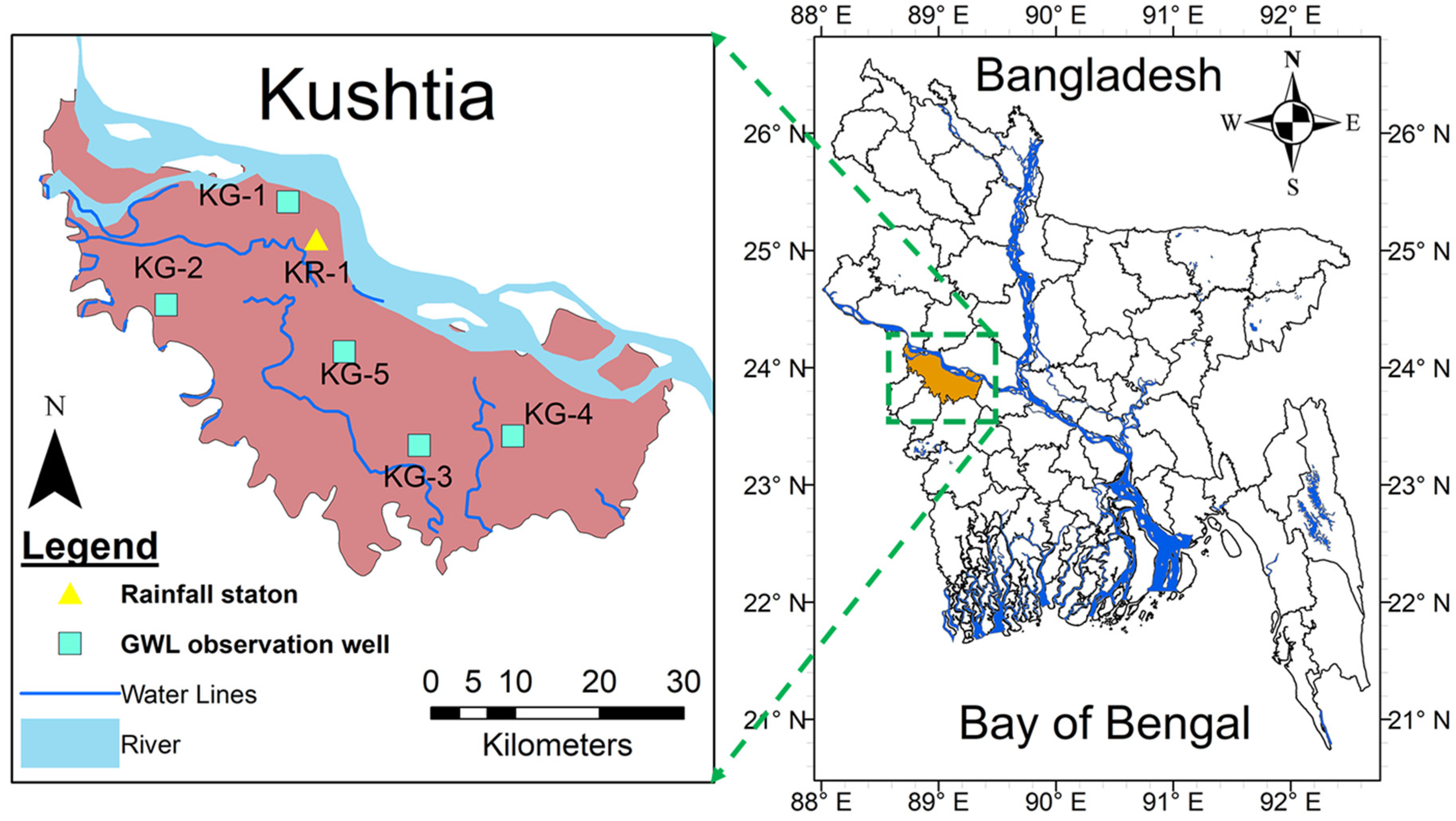
Figure 2.
The sigmoid function.
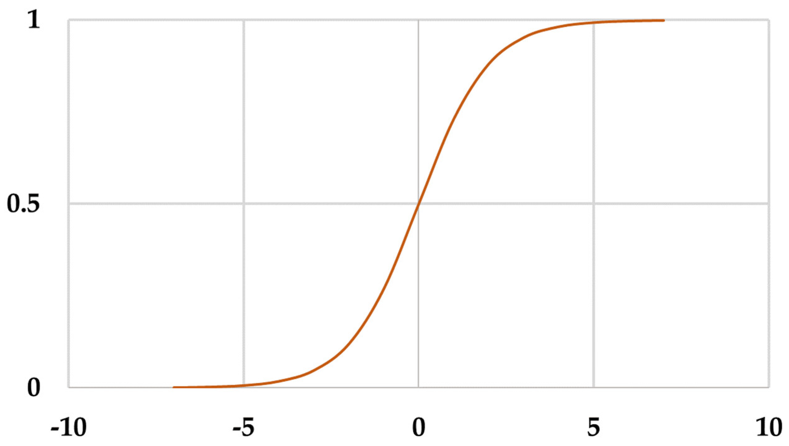
Figure 3.
The ANN model architecture adopted in the current study.
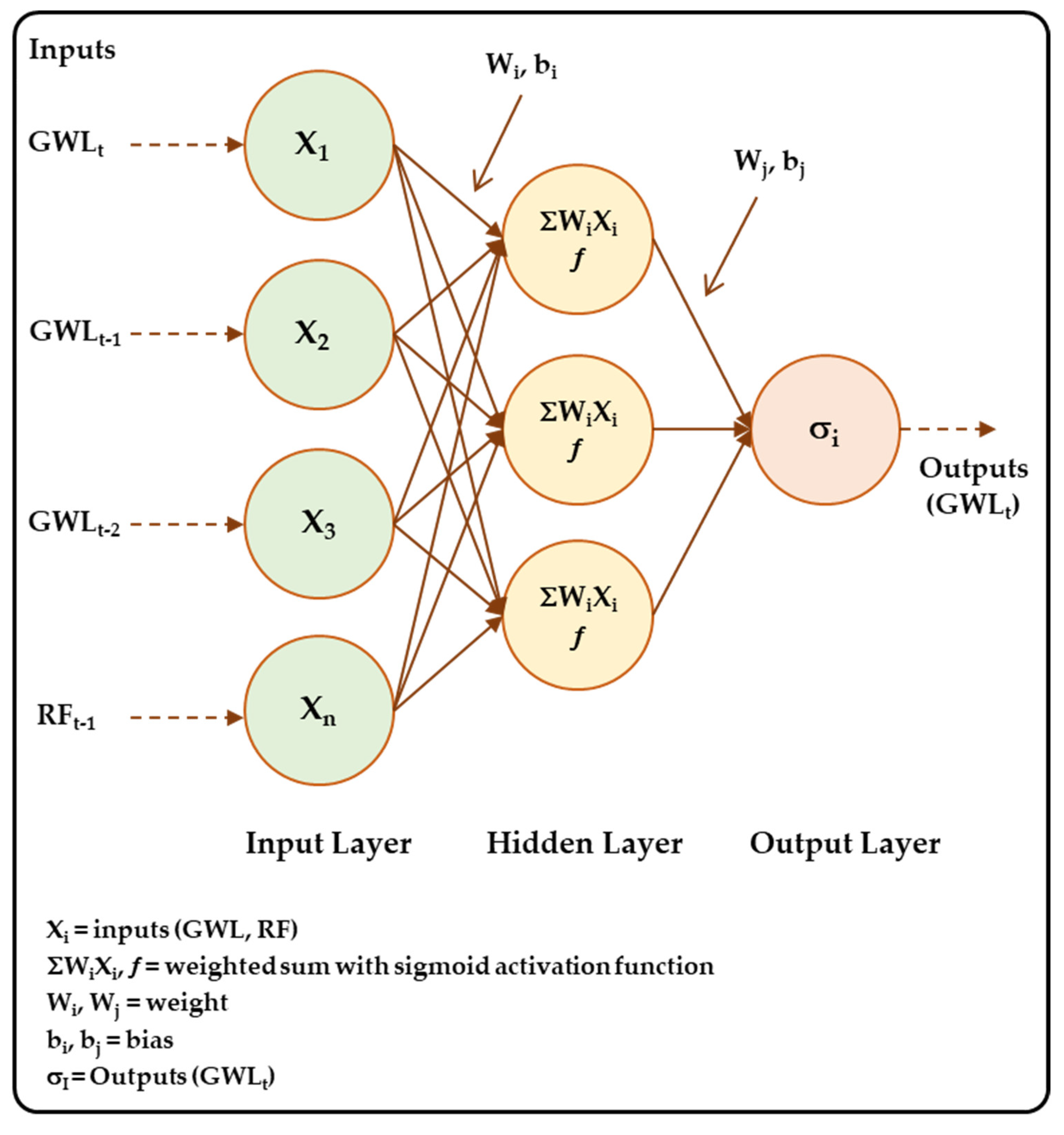
Figure 4.
ARIMA Based Model Building Process.
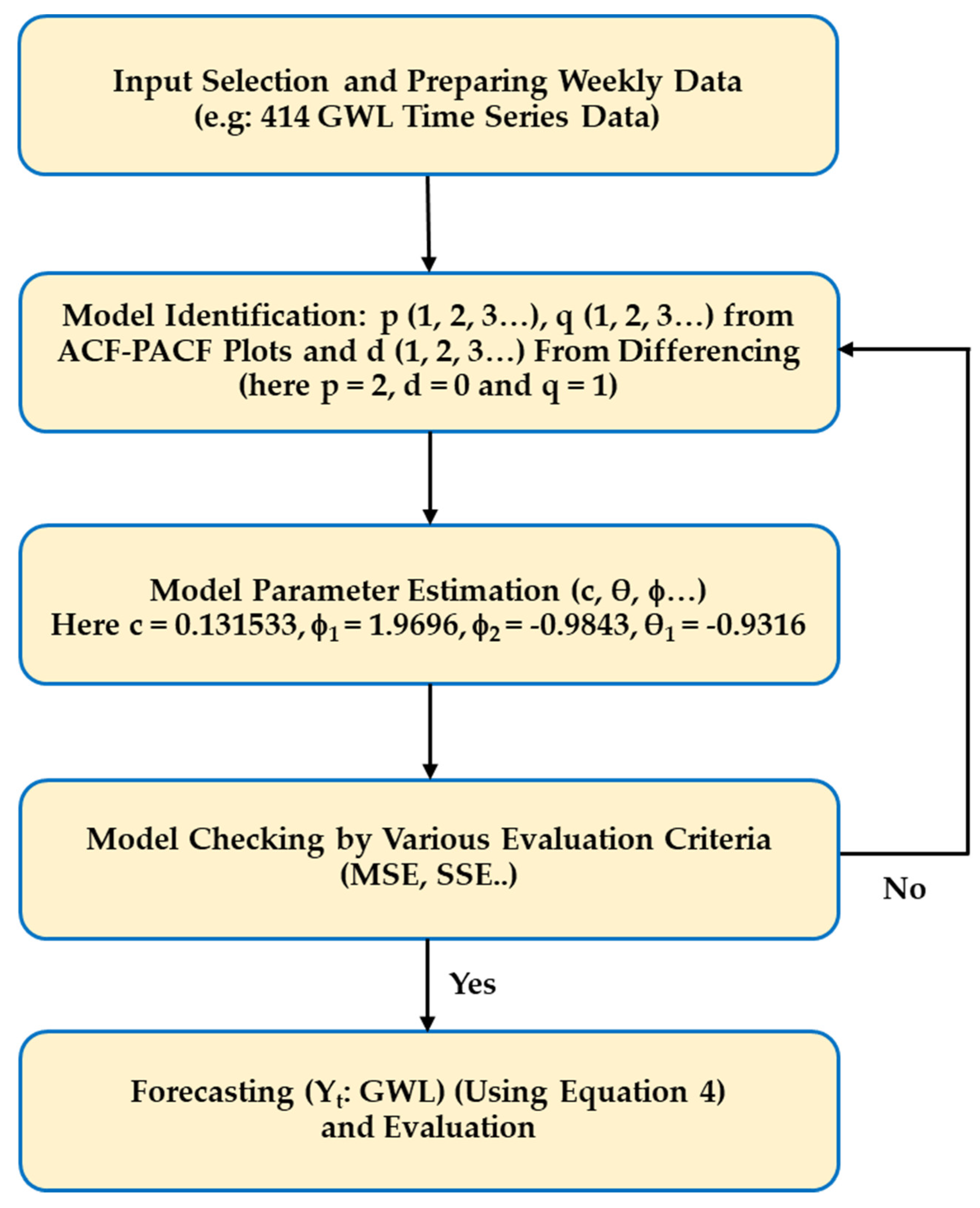
Figure 5.
(a) ACF and (b) PACF plots for GWL fluctuation of Station ID: KG-1, Location: Bheramara.
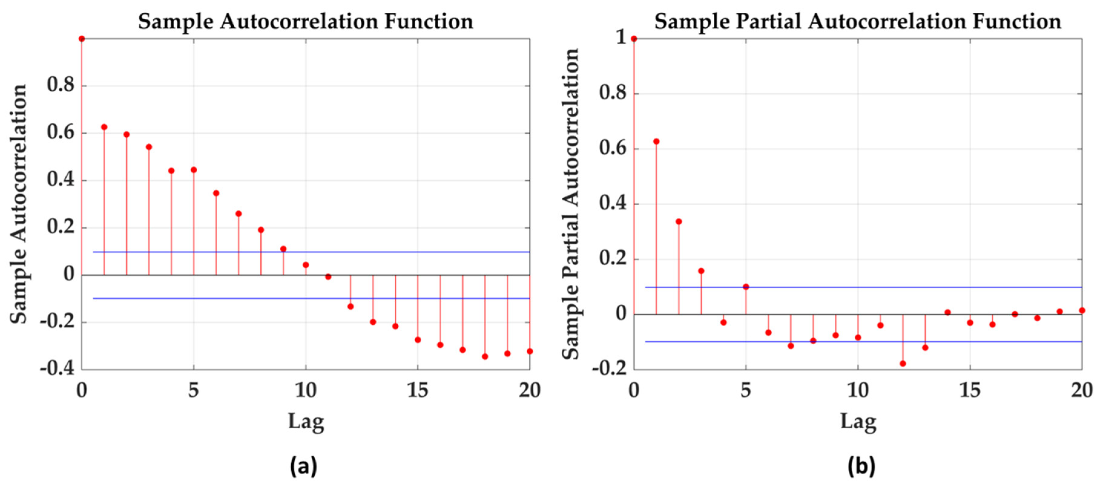
Figure 6.
(a) Scatterplot and (b) Actual and Predicted GWL plot based on the ANN 8-9-1 model for Station ID: KG-5, Location: Mirpur.
Figure 6.
(a) Scatterplot and (b) Actual and Predicted GWL plot based on the ANN 8-9-1 model for Station ID: KG-5, Location: Mirpur.
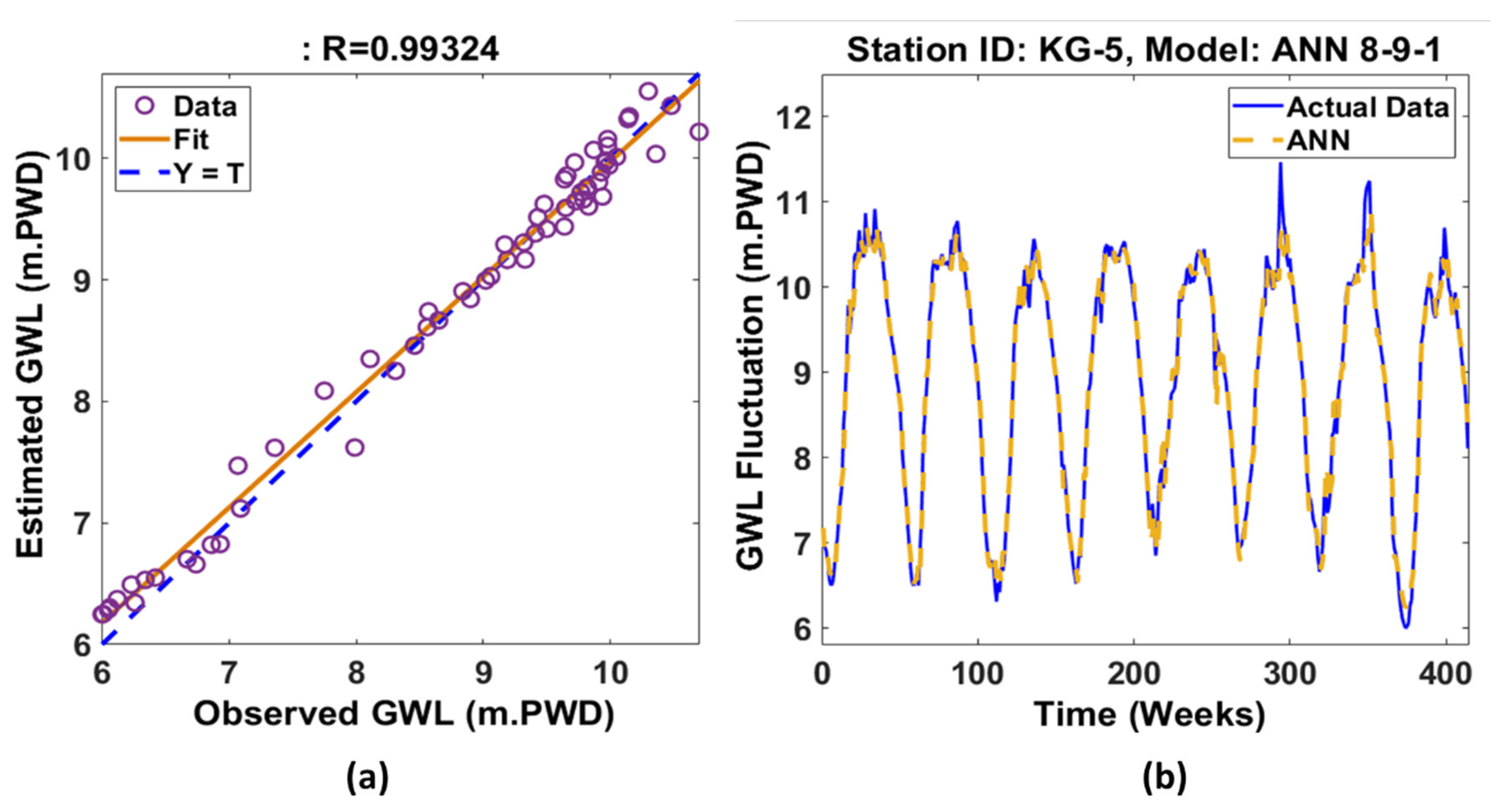
Figure 7.
(a) ACF; (b) PACF; (c) QQ plot; (d) Histogram; (e) Actual and model prediction; (f) Residuals based on ARIMA (2,0,1) model for GWL prediction of Station ID: KG-5: Location: Mirpur.
Figure 7.
(a) ACF; (b) PACF; (c) QQ plot; (d) Histogram; (e) Actual and model prediction; (f) Residuals based on ARIMA (2,0,1) model for GWL prediction of Station ID: KG-5: Location: Mirpur.
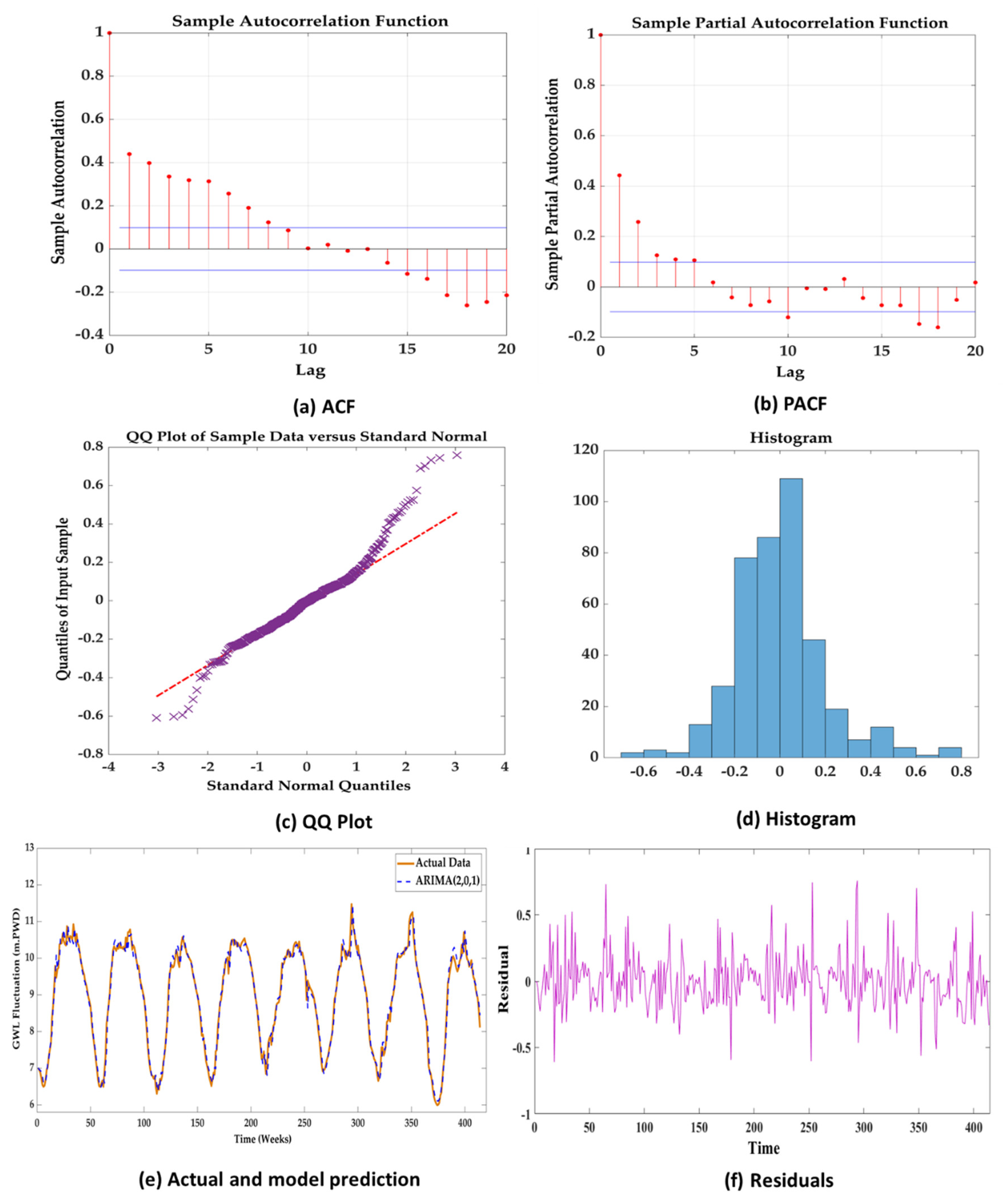
Figure 8.
Existing and predicted GWL based on (a) ARIMAX (3,0,2), Station ID: KG-5, Location: Mirpur and (b) ANN 6-8-1, Station ID: KG-1, Location: Bheramara.
Figure 8.
Existing and predicted GWL based on (a) ARIMAX (3,0,2), Station ID: KG-5, Location: Mirpur and (b) ANN 6-8-1, Station ID: KG-1, Location: Bheramara.
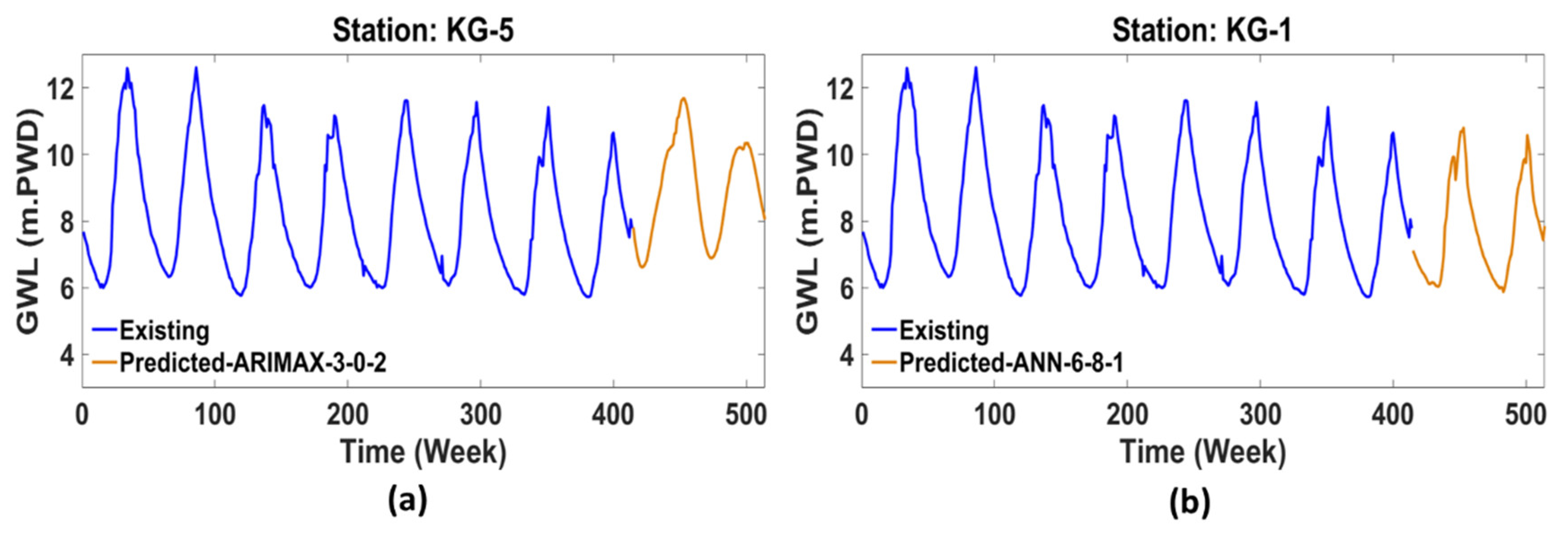

Table 1.
GWL and RF station details.
| SL No |
Station ID |
Station Type |
Location of Station (Sub-District Name) | Latitude (Degree) |
Longitude (Degree) |
|---|---|---|---|---|---|
| 1 | KG-1 | GWL | Bheramara | 24.09 | 88.96 |
| 2 | KG-2 | GWL | Daulatpur | 23.98 | 88.83 |
| 3 | KG-3 | GWL | Kushtia Sadar | 23.83 | 89.10 |
| 4 | KG-4 | GWL | Kumarkhali | 23.84 | 89.20 |
| 5 | KG-5 | GWL | Mirpur | 23.93 | 89.02 |
| 6 | KR-1 | RF | Mirpur | 24.05 | 88.99 |
Table 2.
Performance of the best selected ANN (multivariate) model.
| Station ID | Model Architecture | Model Performance | ||
|---|---|---|---|---|
| RMSE | NSE | SSE | ||
| KG-1 | ANN 6-8-1 | 0.1546 | 0.988 | 9.894 |
| KG-2 | ANN 7-8-1 | 0.1688 | 0.979 | 11.799 |
| KG-3 | ANN 10-4-1 | 0.2319 | 0.965 | 26.910 |
| KG-4 | ANN 6-7-1 | 0.2550 | 0.986 | 22.273 |
| KG-5 | ANN 8-9-1 | 0.1801 | 0.984 | 13.434 |
Table 3.
Performance of the best selected ANN (univariate) model.
| Station ID | Model Architecture | Model Performance | ||
|---|---|---|---|---|
| RMSE | NSE | SSE | ||
| KG-1 | ANN 3-7-1 | 0.1616 | 0.987 | 10.809 |
| KG-2 | ANN 2-3-1 | 0.1715 | 0.979 | 12.171 |
| KG-3 | ANN 4-9-1 | 0.2588 | 0.957 | 26.802 |
| KG-4 | ANN 2-4-1 | 0.2544 | 0.986 | 27.725 |
| KG-5 | ANN 5-10-1 | 0.1812 | 0.9841 | 13.595 |
Table 4.
Performance of the selected ANN (multivariate) models for Station ID: KG-5.
| Model | Training | Validation | Test | |||
|---|---|---|---|---|---|---|
| MSE | NSE | MSE | NSE | MSE | NSE | |
| ANN 8-2-1 | 0.030 | 0.984 | 0.066 | 0.964 | 0.046 | 0.978 |
| ANN 8-3-1 | 0.032 | 0.982 | 0.061 | 0.967 | 0.045 | 0.978 |
| ANN 8-4-1 | 0.046 | 0.975 | 0.069 | 0.963 | 0.076 | 0.963 |
| ANN 8-5-1 | 0.036 | 0.980 | 0.074 | 0.960 | 0.037 | 0.982 |
| ANN 8-6-1 | 0.031 | 0.983 | 0.078 | 0.958 | 0.042 | 0.980 |
| ANN 8-7-1 | 0.030 | 0.983 | 0.201 | 0.892 | 0.040 | 0.981 |
| ANN 8-8-1 | 0.035 | 0.981 | 0.079 | 0.958 | 0.042 | 0.980 |
| ANN 8-9-1 | 0.032 | 0.983 | 0.083 | 0.955 | 0.032 | 0.984 |
| ANN 8-10-1 | 0.027 | 0.985 | 0.071 | 0.962 | 0.039 | 0.981 |
Table 5.
Selected best ARIMAX model results.
| Station ID | Model Architecture | Model Performance (SSE) |
|---|---|---|
| KG-1 | ARIMAX (3,0,3) | 15.361 |
| KG-2 | ARIMAX (3,0,2) | 18.721 |
| KG-3 | ARIMAX (1,0,3) | 25.449 |
| KG-4 | ARIMAX (2,0,0) | 63.680 |
| KG-5 | ARIMAX (3,0,2) | 15.143 |
Table 6.
Selected best ARIMA model results.
| Station ID | Model Architecture | Model Performance (SSE) |
|---|---|---|
| KG-1 | ARIMA (2,0,1) | 17.217 |
| KG-2 | ARIMA (2,0,1) | 26.880 |
| KG-3 | ARIMA (2,0,3) | 28.207 |
| KG-4 | ARIMA (3,0,1) | 64.582 |
| KG-5 | ARIMA (2,0,1) | 16.585 |
Table 7.
Performance of the selected ARIMA (p, d, q) models for Station ID: KG-5.
| Model | SSE | MSE | RMSE | AIC | BIC |
|---|---|---|---|---|---|
| ARIMA (0,2,1) | 20.688 | 0.050 | 0.224 | -59.599 | -47.521 |
| ARIMA (1,2,2) | 20.688 | 0.050 | 0.224 | -55.600 | -35.471 |
| ARIMA (1,2,3) | 20.680 | 0.050 | 0.223 | -53.750 | -29.594 |
| ARIMA (2,0,0) | 21.220 | 0.051 | 0.226 | -47.077 | -30.974 |
| ARIMA (2,0,1) | 16.585 | 0.040 | 0.200 | -147.100 | -126.971 |
| ARIMA (2,0,2) | 16.519 | 0.040 | 0.200 | -146.764 | -122.609 |
| ARIMA (3,0,1) | 16.537 | 0.040 | 0.200 | -146.317 | -122.162 |
| ARIMA (3,2,1) | 20.627 | 0.050 | 0.223 | -54.820 | -30.665 |
| ARIMA (3,2,2) | 20.563 | 0.050 | 0.223 | -54.092 | -25.911 |
| ARIMA (3,2,3) | 20.021 | 0.048 | 0.220 | -63.151 | -30.944 |
Table 8.
Model Parameters for ARIMA (2,0,1) (Station ID: KG-5).
| Parameters | Value | Standard Error | T Statistic | P Value |
|---|---|---|---|---|
| Constant | 0.131533 | 0.009164 | 14.35275 | 1.02×10-46 |
| AR{1} | 1.969639 | 0.008054 | 244.5408 | 0 |
| AR{2} | -0.98431 | 0.007999 | -123.057 | 0 |
| MA{1} | -0.93165 | 0.020288 | -45.9215 | 0 |
| Variance | 0.040065 | 0.002092 | 19.1474 | 1.02×-81 |
Table 9.
Predicted highest, lowest, and average GWL values.
| Station ID | Model/Data | Highest (m.PWD) |
Lowest (m.PWD) |
Average (m.PWD) |
|---|---|---|---|---|
| KG-1 | Existing raw data | 12.610 | 5.730 | 8.148 |
| KG-1 | ANN 6-8-1 (MV) | 10.797 | 5.875 | 7.742 |
| KG-5 | ARIMAX (3,0,2) | 11.694 | 6.622 | 8.951 |
Table 10.
Evaluation Metrics and Comparative Performance Improvement of the Predictive Models.
| Improvement in Performance (ΔPE, ΔPD or BRM) |
Remarks | ||||||
|---|---|---|---|---|---|---|---|
| Station ID | Results (SSE) |
Model Architecture | ANN (MV) (%) |
ANN (UV) (%) |
ARIMAX (%) |
ARIMA (%) |
|
| KG-1 | 9.89 | ANN 6-8-1 (MV) | 0 (BRM) | -8.45 (∆PD) |
-34.65 (∆PD) |
-40.34 (∆PD) | In contrast to ANN(MV) ΔPE: -, ∆PD: ANN (UV), ARIMAX, ARIMA; |
| KG-1 | 10.80 | ANN 3-7-1 (UV) | 9.24 (∆PE) |
0 (BRM) | -28.62 (∆PD) |
-34.82 (∆PD) | In contrast to ANN (UV) ΔPE: ANN (MV), ∆PD: ARIMAX, ARIMA; |
| KG-5 | 15.14 | ARIMAX (3,0,2) | 53.04 (∆PE) | 40.09 (∆PE) | 0 (BRM) |
-8.69 (∆PD) | In contrast to ARIMAX ΔPE: ANN (MV), ANN (UV), ∆PD: ARIMA; |
| KG-1 | 16.58 | ARIMA (2,0,1) | 67.61 (∆PE) | 53.43 (∆PE) | 9.52 (∆PE) |
0 (BRM) |
In contrast to ARIMA ΔPE: ANN (MV), ANN (UV), ARIMAX ∆PD: -; |
Disclaimer/Publisher’s Note: The statements, opinions and data contained in all publications are solely those of the individual author(s) and contributor(s) and not of MDPI and/or the editor(s). MDPI and/or the editor(s) disclaim responsibility for any injury to people or property resulting from any ideas, methods, instructions or products referred to in the content. |
© 2024 by the authors. Licensee MDPI, Basel, Switzerland. This article is an open access article distributed under the terms and conditions of the Creative Commons Attribution (CC BY) license (http://creativecommons.org/licenses/by/4.0/).
Copyright: This open access article is published under a Creative Commons CC BY 4.0 license, which permit the free download, distribution, and reuse, provided that the author and preprint are cited in any reuse.


