Submitted:
02 October 2024
Posted:
03 October 2024
You are already at the latest version
Abstract
Keywords:
1. Introduction
2. Literature Review
3. Research Method
- Project Type (e.g., schools, hostels, industrial buildings)
- Number of Projects (for each type)
- Average Project Duration (in months)
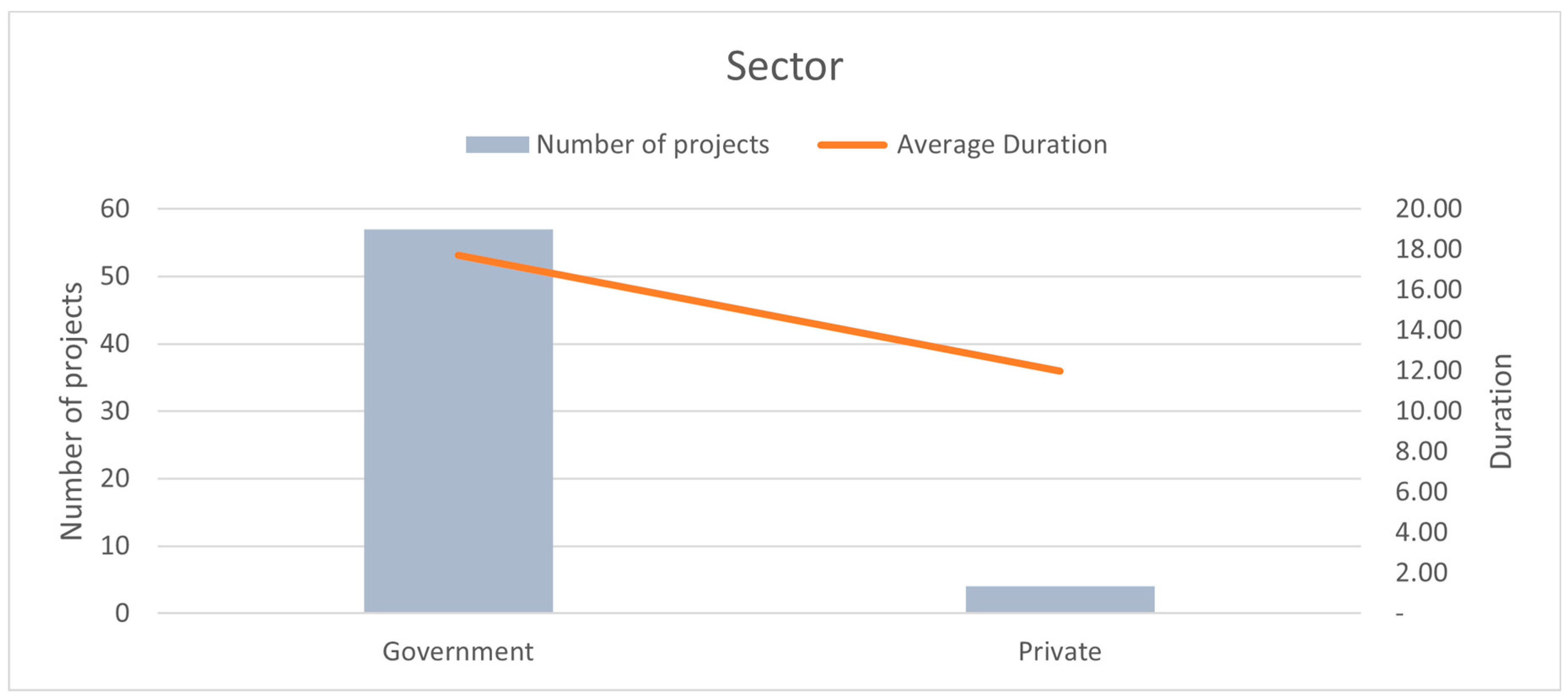
- Sector (Government or Private)
- Extension Indicator (whether the project required an extension or not)
4. Results and Discussion
- 4.1 Province-Based Duration Variability
- ANOVA Results
5. Conclusions, Implications and Recommendations
6. Limitations and Areas for Future Studies
Author Contributions
Data Availability Statement
Conflicts of Interest
References
- Rizaee, S.; Lei, Z. Duration Estimation of a Heavy Industrial Scaffolding Project: A Case Study. J. Constr. Eng. Manag. 2024, 150. [Google Scholar] [CrossRef]
- ElMenshawy, M.; Marzouk, M. Automated BIM Schedule Generation Approach for Solving Time–Cost Trade-off Problems. Eng. Constr. Archit. Manag. 2021, 28, 3346–3367. [Google Scholar] [CrossRef]
- Abeyasinghe, M. C. L.; Greenwood, D. J.; Johansen, D. E. An Efficient Method for Scheduling Construction Projects with Resource Constraints. Int. J. Proj. Manag. 2001, 19, 29–45. [Google Scholar] [CrossRef]
- Nevett, G.; Goodrum, P. M.; Littlejohn, R. L. Understanding the Effect of Bid Quantities, Project Characteristics, and Project Locations on the Duration of Road Transportation Construction Projects during Early Stages. Transp. Res. Rec. 2020, 2675, 121–134. [Google Scholar] [CrossRef]
- Sadeghi, N.; Dehghani, M. S.; Ingolfsson, A. Choice of Probability Distributions for Activity Durations in Project Networks with Limited Sample Size. J. Constr. Eng. Manag. 2024, 150. [Google Scholar] [CrossRef]
- Vandevoorde, S.; Vanhoucke, M. A Comparison of Different Project Duration Forecasting Methods Using Earned Value Metrics. Int. J. Proj. Manag. 2006, 24, 289–302. [Google Scholar] [CrossRef]
- Akin, F. D.; Damci, A.; Arditi, D. Optimum Finance-Based Scheduling. J. Constr. Eng. Manag. 2024, 150. [Google Scholar] [CrossRef]
- Laryea, S.; Watermeyer, R.; Govender, N. The Influence of Fees on the Quality of Professional Services in South Africa. In Proceedings of the Institution of Civil Engineers - Management, Procurement and Law; 2020. [CrossRef]
- Ballesteros-Pérez, P.; Smith, S. T.; Lloyd-Papworth, J. G.; Cooke, P. Incorporating the Effect of Weather in Construction Scheduling and Management with Sine Wave Curves: Application in the United Kingdom. Constr. Manag. Econ. 2018, 36, 666–682. [Google Scholar] [CrossRef]
- Yang, J.-B.; Chen, Y.-H. Enhanced ESM Approach for Duration Forecasting in Delayed Projects. Ain Shams Eng. J. 2024, 15. [Google Scholar] [CrossRef]
- Al Haj, R. A.; El-Sayegh, S. M. Time-Cost Optimization Model Considering Float-Consumption Impact. J. Constr. Eng. Manag. 2015, 141. [Google Scholar] [CrossRef]
- Mahdi Hosseinian, S.; Arjomand, A.; Li, C. Q.; Zhang, G. Developing a Model for Assessing Project Completion Time Reliability during Construction Using Time-Dependent Reliability Theory. J. Constr. Eng. Manag. 2022, 148. [Google Scholar] [CrossRef]
- Diamantas, V. K.; Kirytopoulos, K. A.; Leopoulos, V. N. Project’s Duration Prediction: Traditional Tools or Simulation? World Rev. Entrep. Manag. Sustain. Dev. 2007, 3, 317–333. [Google Scholar] [CrossRef]
- Bhardwaj, M.; Rana, A.; Sharma, N. K. How Software Size Influence Productivity and Project Duration. Int. J. Electr. Comput. Eng. 2019, 9, 2006–2017. [Google Scholar] [CrossRef]
- Koulinas, G. K.; Xanthopoulos, A. S.; Tsilipiras, T. T.; Koulouriotis, D. E. Schedule Delay Risk Analysis in Construction Projects with a Simulation-Based Expert System. Buildings 2020, 10. [Google Scholar] [CrossRef]
- Zeng, X.; Yu, Y.; Yang, S.; Lv, Y.; Sarker, M. N. I. Urban Resilience for Urban Sustainability: Concepts, Dimensions, and Perspectives. Sustain. 2022, 14. [Google Scholar] [CrossRef]
- van Niekerk, J.; Wium, J.; de Koker, N. The Value of Data from Construction Project Site Meeting Minutes in Predicting Project Duration. Built Environ. Proj. Asset Manag. 2022, 12, 738–753. [Google Scholar] [CrossRef]
- Hegab, M. Y.; Smith, G. R. Delay Time Analysis in Microtunneling Projects. J. Constr. Eng. Manag. 2007, 133, 191–195. [Google Scholar] [CrossRef]
- Barrientos-Orellana, A.; Ballesteros-Pérez, P.; Mora-Melia, D.; González-Cruz, M. C.; Vanhoucke, M. Stability and Accuracy of Deterministic Project Duration Forecasting Methods in Earned Value Management. Eng. Constr. Archit. Manag. 2022, 29, 1449–1469. [Google Scholar] [CrossRef]
- Hasan, M. F.; Mohammed, S. R. Factors Affecting Time and Cost Trade-off in Multiple Construction Projects. Arch. Civ. Eng. 2022, 68, 549–561. [Google Scholar] [CrossRef]
- Irwanto, R.; Rahayu, T.; Panudju, A. T. Artificial Neural Networks for Construction Project Cost and Duration Estimation. Rev. d’Intelligence Artif. 2023, 37, 1449–1460. [Google Scholar] [CrossRef]
- Ballesteros-Pérez, P.; Cerezo-Narváez, A.; Otero-Mateo, M.; Pastor-Fernández, A.; Zhang, J.; Vanhoucke, M. Forecasting the Project Duration Average and Standard Deviation from Deterministic Schedule Information. Appl. Sci. 2020, 10. [Google Scholar] [CrossRef]
- Maharaj, R.; Musonda, I.; Onososen, A. Construction Organisation’s Planning and Implementation: The Case Between Conceptualization and Implementation Teams. Springer 2023, 245. [Google Scholar] [CrossRef]
- Mahamid, I. Analysis of Schedule Deviations in Road Construction Projects and the Effects of Project Physical Characteristics: J. Financ. Manag. Prop. Constr. 2017, 22, 192–210. [Google Scholar] [CrossRef]
- Kim, Y.; Asce, S. M.; Kim, H.; Asce, M.; Murphy, R.; Lee, S.; Asce, M.; Ahn, C. R.; Asce, A. M. Delegation or Collaboration : Understanding Different Construction Stakeholders ’ Perceptions of Robotization. J. Manag. Eng 2022, 38, 1–12. [Google Scholar] [CrossRef]
- Lee, J.; Hyun, H. Multiple Modular Building Construction Project Scheduling Using Genetic Algorithms. J. Constr. Eng. Manag. 2019, 145. [Google Scholar] [CrossRef]
- Babalola, J.; Onososen, A. O. Quantity Surveyors’ Competencies in the Emerging Green Building Adoption. Lagos J. Environ. Stud. 2022, 11, 52–60. [Google Scholar]
- Sapti, M.; Pancapalaga, W.; Widari, W. Managing Risk of Construction Projects to Enhance Project Performance Delivery. J. Sains dan Seni ITS 2019, 53, 1689–1699. [Google Scholar]
- Onososen, A. O.; Musonda, I.; Moyo, T.; Muzioreva, H. Digital Twin Technology in Health, Safety, and Wellbeing Management in the Built Environment. In Smart and Resilient Infrastructure For Emerging Economies: Perspectives on Building Better; Musonda, I., Mwanaumo, E., Onososen, A., Moyo, T., Eds.; CRC Press LLC, 2024; p 7. [CrossRef]
- Kazaz, A.; Ulubeyli, S.; Tuncbilekli, N. A. Causes of Delays in Construction Projects in Turkey. J. Civ. Eng. Manag. 2012, 18, 426–435. [Google Scholar] [CrossRef]
- Ferlito, T.-L.; Musonda, I.; Tjebane, M. M.; Onososen, A. O. Systematic Literature Review on Sustainable Construction Strategies for the Development of Affordable Housing. In The Twelfth International Conference on Construction in the 21st Century (CITC-12; 2022; pp 195–203.
- Fagbenro, R.; Oyediran, O. S.; Onososen, A. O. Consulting Business Workflow and Design Performance Metrics for BIM Based Construction Design in Nigeria. ECS Trans. 2022, 107, 1029. [Google Scholar] [CrossRef]
- Oruc, S.; Dikbas, H. A.; Gumus, B.; Yucel, I. The Impact of Climate Change on Construction Activity Performance. Buildings 2024, 14. [Google Scholar] [CrossRef]
- Little, R. G.; Loggins, R. A.; Wallace, W. A. Building the Right Tool for the Job: Value of Stakeholder Involvement When Developing Decision-Support Technologies for Emergency Management. Nat. Hazards Rev. 2015, 16. [Google Scholar] [CrossRef]
- Lin, J. C.-W.; Lv, Q.; Yu, D.; Srivastava, G.; Chen, C.-H. Optimized Scheduling of Resource-Constraints in Projects for Smart Construction. Inf. Process. Manag. 2022, 59. [Google Scholar] [CrossRef]
- Zwikael, O.; Cohen, Y.; Sadeh, A. Non-Delay Scheduling as a Managerial Approach for Managing Projects. Int. J. Proj. Manag. 2006, 24, 330–336. [Google Scholar] [CrossRef]
- Turkoglu, H.; Polat, G.; Akin, F. D. Crashing Construction Projects Considering Schedule Flexibility: An Illustrative Example. Int. J. Constr. Manag. 2023, 23, 619–628. [Google Scholar] [CrossRef]
- Musonda, I.; Onososen, A. O.; Moyo, T.; Tjebane, M. M. COVID-19 and Shock Events in the AEC Sector-Perspectives on Mitigating Measures. In Construction Safety, Health and Well-being in the COVID-19 era; Manu, P., Cheung, C., Yunusa-Kaltungo, A., Emuze, F., Saurin, T. A., Hadikusumo, B. H. W., Eds.; Routledge: New York, 2023. [Google Scholar] [CrossRef]
- Moyanga, D.; Ojo, L. D.; Awodele, O. A.; Ogunsemi, D. R. Prioritizing the Survival Determinants of Quantity Surveying Firms in Economic Contraction. Eng. Constr. Archit. Manag. 2023. [Google Scholar] [CrossRef]
- Ogunsemi, D. R.; Jagboro, G. O. Time-Cost Model for Building Projects in Nigeria. Constr. Manag. Econ. 2006, 24, 253–258. [Google Scholar] [CrossRef]
- Tjebane, M. M.; Musonda, I.; Onososen, A.; Ramabodu, M. Challenges for the Implementation of Sustainable Construction Practices in Developing Countries: A Bibliometric. In Advances in Information Technology in Civil and Building Engineering: Proceedings of ICCCBE 2022-Volume 2; 2023; p 109. [CrossRef]
- Pawan, P.; Lorterapong, P. A Fuzzy-Based Integrated Framework for Assessing Time Contingency in Construction Projects. J. Constr. Eng. Manag. 2016, 142. [Google Scholar] [CrossRef]
- Ren, L.; Li, P.-P.; Zhao, Y.-G. An Efficient and Effective Method for Reliability Assessment of Project Duration. Qual. Technol. Quant. Manag. 2023, 20, 689–706. [Google Scholar] [CrossRef]
- Berlin, S.; Raz, T.; Glezer, C.; Zviran, M. Comparison of Estimation Methods of Cost and Duration in IT Projects. Inf. Softw. Technol. 2009, 51, 738–748. [Google Scholar] [CrossRef]
- Abdelbasset, E.; Hassan, A.; Amer, N. H.; Khalifa, Y. A. Optimizing the Number of Crews Working in Parallel and Their Work Sequence to Minimize Project Duration and Cost for Repetitive Construction Projects. Innov. Infrastruct. Solut. 2023, 8. [Google Scholar] [CrossRef]
- Le, C.; Jeong, H. D. Determining Highway Project Contract Time from Project Duration Estimates. J. Leg. Aff. Disput. Resolut. Eng. Constr. 2023, 15. [Google Scholar] [CrossRef]
- Malik, T. H. Temporal and Social Distances of the Estimated Duration of R&D Projects in the Biopharma Industry. Technol. Forecast. Soc. Change 2024, 208. [Google Scholar] [CrossRef]
- Jaśkowski, P.; Sobotka, A. Scheduling Construction Projects Using Evolutionary Algorithm. J. Constr. Eng. Manag. 2006, 132, 861–870. [Google Scholar] [CrossRef]
- Ock, J.-H.; Han, S.-H. Measuring Risk-Associated Activity’s Duration: A Fuzzy Set Theory Application. KSCE J. Civ. Eng. 2010, 14, 663–671. [Google Scholar] [CrossRef]
- Arabpour Roghabadi, M.; Moselhi, O. Optimized Crew Selection for Scheduling of Repetitive Projects. Eng. Constr. Archit. Manag. 2020, 28, 1517–1540. [Google Scholar] [CrossRef]
- Türkakın, O. H.; Manisalı, E.; Arditi, D. Delay Analysis in Construction Projects with No Updated Work Schedules. Eng. Constr. Archit. Manag. 2020, 27, 2893–2909. [Google Scholar] [CrossRef]
- Ballesteros-Pérez, P.; Sanz-Ablanedo, E.; Cerezo-Narváez, A.; Lucko, G.; Pastor-Fernández, A.; Otero-Mateo, M.; Contreras-Samper, J. P. Forecasting Accuracy of In-Progress Activity Duration and Cost Estimates. J. Constr. Eng. Manag. 2020, 146. [Google Scholar] [CrossRef]
- Mulenga, M. J. Explaining Cost Overruns on Construction Projects in Gauteng Province, South Africa. 2016.
- Riedel, E.; Al-Keim, A. Strategies to Reduce Cost Overruns and Schedule Delays in Construction Projects. Walden Diss. Dr. Stud. 2017, 159. [Google Scholar]
- Youssefi, I.; Celik, T. Optimized Approach toward Identification of Influential Cost Overrun Causes in Construction Industry. ASCE-ASME J. Risk Uncertain. Eng. Syst. Part A Civ. Eng. 2023, 9. [Google Scholar] [CrossRef]
- Nuako, F.; Ghansah, F. A.; Adusei, T. Critical Success Factorsfor Cost Overrun Minimization in Public Construction Projects in Developing Countries: The Case of Ghana. Constr. Innov. 2024. [Google Scholar] [CrossRef]
- Famiyeh, S.; Amoatey, C. T.; Adaku, E.; Agbenohevi, C. S. Major Causes of Construction Time and Cost Overruns: A Case of Selected Educational Sector Projects in Ghana. J. Eng. Des. Technol. 2017, 15, 181–198. [Google Scholar] [CrossRef]
- Sweis, G. J. Factors Affecting Time Overruns in Public Construction Projects: The Case of Jordan. Int. J. Bus. Manag. 2013, 8, 120–129. [Google Scholar] [CrossRef]
- Dzvimbo, M. A.; Mashizha, T. M.; Zhanda, K.; Mawonde, A. Promoting Sustainable Development Goals: Role of Higher Education Institutions in Climate and Disaster Management in Zimbabwe. Jamba J. Disaster Risk Stud. 2022, 14. [Google Scholar] [CrossRef]
- Mulalo, R.; Ibrahimu, K.; Nwobodo-Anyadiegwu, E. Project Cost Overrun in the South African Construction Sector: A Case Study of Johannesburg Metropolis. Proc. Int. Conf. Ind. Eng. Oper. Manag. 2018, 2018, 1263–1270. [Google Scholar]
- Sinesilassie, E. G.; Tabish, S. Z. S.; Jha, K. N. Critical Factors Affecting Schedule Performance. Eng. Constr. Archit. Manag. 2017, 24, 757–773. [Google Scholar] [CrossRef]
- Annamalaisami, C. D.; Kuppuswamy, A. Managing Cost Risks: Toward a Taxonomy of Cost Overrun Factors in Building Construction Projects. ASCE-ASME J. Risk Uncertain. Eng. Syst. Part A Civ. Eng. 2021, 7. [Google Scholar] [CrossRef]
- Mabaso, M. Risk Identification in Megaprojects and Its Impacts on Project Management Constraints in Civil Engineering and Construction Companies. 2022, No. November.
- Gunduz, M.; Nielsen, Y.; Ozdemir, M. Fuzzy Assessment Model to Estimate the Probability of Delay in Turkish Construction Projects. J. Manag. Eng. 2015, 31. [Google Scholar] [CrossRef]
- Onososen, A. O.; Musonda, I.; Onatayo, D.; Tjebane, M. M.; Saka, A. B.; Fagbenro, R. K. Impediments to Construction Site Digitalisation Using Unmanned Aerial Vehicles (UAVs). Drones 2023, 7, 45. [Google Scholar] [CrossRef]
- Mukuka, M.; Aigbavboa, C.; Thwala, W. Understanding Construction Projects’ Schedule Overruns in South Africa. ICCREM 2015 - Environ. Sustain. Build. - Proc. 2015 Int. Conf. Constr. Real Estate Manag. 2015, 591–602. [CrossRef]
- Gondia, A.; Siam, A.; El-Dakhakhni, W.; Nassar, A. H. Machine Learning Algorithms for Construction Projects Delay Risk Prediction. J. Constr. Eng. Manag. 2020, 146, 1–16. [Google Scholar] [CrossRef]
- Oshungade, Oluwaseun Olumide, D. K. A Comparative Study of Causes and Effects of Project Delays and Disruptions in Construction Projects in the South African Construction Industry : City of Johannesburg As a Case Study. 2016, 168.
- Wang, X.; Wang, X.; Huang, Y. Chinese Construction Worker Reluctance toward Vocational Skill Training. J. Eng. Des. Technol. 2019, 17, 155–171. [Google Scholar] [CrossRef]
- Szewczyk, B.; Radziszewska-Zielina, E. IT-Based Control and Assessment of Partnering Relations in Construction Projects. Autom. Constr. 2020, 116. [Google Scholar] [CrossRef]
- Maltese, S.; Tagliabue, L. C.; Cecconi, F. R.; Pasini, D.; Manfren, M.; Ciribini, A. L. C. Sustainability Assessment through Green BIM for Environmental, Social and Economic Efficiency. Procedia Eng. 2017, 180, 520–530. [Google Scholar] [CrossRef]
- Olawumi, T. O.; Chan, D. W. M. Developing Project Evaluation Models for Smart Sustainable Practices Implementation in Construction Projects: A Comparative Study between Nigeria and Hong Kong. Eng. Constr. Archit. Manag. 2022, 29, 1522–1552. [Google Scholar] [CrossRef]
- Malkina, M.; Rogachev, D. Financial Contagion of Russian Companies during the COVID-19 Pandemic. J. Corp. Financ. Res. 2023, 17, 55–71. [Google Scholar] [CrossRef]
- Freeman, J.; Hancock, L. Energy and Communication Infrastructure for Disaster Resilience in Rural and Regional Australia. Reg. Stud. 2017, 51, 933–944. [Google Scholar] [CrossRef]
- Loewenberger, P. A.; Newton, M.; Wick, K. Developing Creative Leadership in a Public Sector Organisation. Int. J. Public Sect. Manag. 2014, 27, 190–200. [Google Scholar] [CrossRef]
- Liphadzi, M.; Musonda, I.; Onososen, A. O. The Use of Building Information Modelling Tools for Effective Waste Management: A Systematic Review. In World Building Congress,IOP Conf. Ser.: Earth Environ. Sci. 1101 062001; IOP, 2022. [CrossRef]
- Rodrigues, I. L. The Role of Construction Companies in Modern Housing. Precol’s Footprint in Late Colonial Angola. In 17th International Docomomo Conference - Modern Design: Social Commitment and Quality of Life, Proceedings; C.J., S., M.P., F., A., T., U., P., Eds.; Docomomo, 2022; pp 276–286.
- Azasu, S.; Adewunmi, Y.; Babatunde, O. South African Stakeholder Views of the Competency Requirements of Facilities Management Graduates. Int. J. Strateg. Prop. Manag. 2018, 22, 471–478. [Google Scholar] [CrossRef]
- Makhathini, N.; Musonda, I.; Onososen, A. Utilisation of Remote Monitoring Systems in Construction Project Management. In Construction in 5D: Deconstruction, Digitalization, Disruption, Disaster, Development.; Haupt, T.C., Akinlolu, M., Simpeh, F., Amoah, C., Armoed, Z., Ed.; Springer, 2023. [CrossRef]
- Akinradewo, O.; Oke, A.; Aigbavboa, C.; Mashangoane, M. Willingness to Adopt Robotics and Construction Automation in the South African Construction Industry. In Proceedings of the International Conference on Industrial Engineering and Operations Management; 2018.
- Ebekozien, A.; Aigbavboa, C.; Samsurijan, M. S.; Radin Firdaus, R. B.; Ayo-Odifiri, S. O.; Amadi, G. C. An Appraisal of Guidelines and Practices for Municipal Infrastructure Support Agent to Execute Labour-Intensive Construction Projects in South Africa. Prop. Manag. 2024, 42, 70–85. [Google Scholar] [CrossRef]
- Ebekozien, A.; Aigbavboa, C. O. Improving Quantity Surveying Education through Continually Updating Curriculum Digitalisation to Meet Industry Requirements. J. Eng. Des. Technol. 2023. [Google Scholar] [CrossRef]
- Manfren, M.; Tagliabue, L. C.; Re Cecconi, F.; Ricci, M. Long-Term Techno-Economic Performance Monitoring to Promote Built Environment Decarbonisation and Digital Transformation—A Case Study. Sustain. 2022, 14. [Google Scholar] [CrossRef]
- Onososen, A. O.; Musonda, I. Research Focus for Construction Robotics and Human-Robot Teams towards Resilience in Construction: Scientometric Review. J. Eng. Des. Technol. 2022. [Google Scholar] [CrossRef]
- Onososen, A.; Musonda, I. Perceived Benefits of Automation and Artificial Intelligence in the AEC Sector: An Interpretive Structural Modeling Approach. Front. Built Environ. 2022, 61. [Google Scholar] [CrossRef]
- Ajayi, A.; Oyedele, L.; Owolabi, H.; Akinade, O.; Bilal, M.; Davila Delgado, J. M.; Akanbi, L. Deep Learning Models for Health and Safety Risk Prediction in Power Infrastructure Projects. Risk Anal. 2020, 40, 2019–2039. [Google Scholar] [CrossRef]
- Tucker, R. L. Japanese Construction Industry. Autom. Constr. 1992, 1, 27–34. [Google Scholar] [CrossRef]
- Onososen, A.; Osanyin, O.; Adeyemo, M. Drivers and Barriers to the Implementation of Green Building Development. PM World J. 2019, 9, 1–15. [Google Scholar]
- Yap, J. B. H.; Skitmore, M.; Lim, Y. W.; Loo, S.-C.; Gray, J. Assessing the Expected Current and Future Competencies of Quantity Surveyors in the Malaysian Built Environment. Eng. Constr. Archit. Manag. 2022, 29, 2415–2436. [Google Scholar] [CrossRef]
- Khanh, H. D.; Kim, S. Y.; Khoa, N. Van; Tu, N. T. The Relationship between Workers’ Experience and Productivity: A Case Study of Brick Masonry Construction. Int. J. Constr. Manag. 2021, 0, 1–10. [Google Scholar] [CrossRef]
- Onososen, A.; Musonda, I.; Ramabodu, M.; Dzuwa, C. Task Performance to Understand the Effectiveness of Visualisation Technology-Based Training for Human-Drone Interaction Learning. In Advances in Information Technology in Civil and Building Engineering. ICCCBE 2022. Lecture Notes in Civil Engineering, vol 358.; Skatulla, S., Beushausen, H., Eds.; Springer Nature Switzerland: Switzerland, 2023; pp 297–310. [CrossRef]
- Yuan, D.; Yau, Y.; Hou, H.; Liu, Y. Factors Influencing the Project Duration of Urban Village Redevelopment in Contemporary China. Land 2021, 10. [Google Scholar] [CrossRef]
- Dixon, R.; McGregor, A. Grassroots Development and Upwards Accountabilities: Tensions in the Reconstruction of Aceh’s Fishing Industry. Dev. Change 2011, 42, 1349–1377. [Google Scholar] [CrossRef]
- Santos, R.; Costa, A. A.; Silvestre, J. D.; Vandenbergh, T.; Pyl, L. BIM-Based Life Cycle Assessment and Life Cycle Costing of an Office Building in Western Europe. Build. Environ. 2020, 169. [Google Scholar] [CrossRef]
- Ju, W.; Wu, J.; Kang, Q.; Jiang, J.; Xing, Z. Fire Risk Assessment of Subway Stations Based on Combination Weighting of Game Theory and TOPSIS Method. Sustain. 2022, 14. [Google Scholar] [CrossRef]
- Hokkeling, J. Towards Construction 4.0: An Assessment on the Potential of Digital Twins in the Infrastructure Sector. Univ. Twente 2020, 1–120.
- Tjebane, M. M.; Musonda, I.; Onososen, A.; Ramabodu, M. Challenges for the Implementation of Sustainable Construction Practices in Developing Countries: A Bibliometric Review. In Advances in Information Technology in Civil and Building Engineering. ICCCBE 2022. Lecture Notes in Civil Engineering, vol 358. Springer,; Skatulla, S., Beushausen: Switzerland, 2023. [CrossRef]
- Bhattacharya, S.; Chatterjee, A. Digital Project Driven Supply Chains: A New Paradigm. Supply Chain Manag. 2021, 2, 283–294. [Google Scholar] [CrossRef]
- Tjebane, M. M.; Musonda, I.; Onososen, A.; Ramabodu, M. Unravelling the State of the Art of Blockchain Development for Improved Infrastructure Delivery in the Built Environment: A Bibliometric Review. In Advances in Information Technology in Civil and Building Engineering. ICCCBE 2022. Lecture Notes in Civil Engineering, vol 358. Springer, Cham; Skatulla, S., Beushausen, H., Eds.; Springer: Switzerland, 2023. [CrossRef]
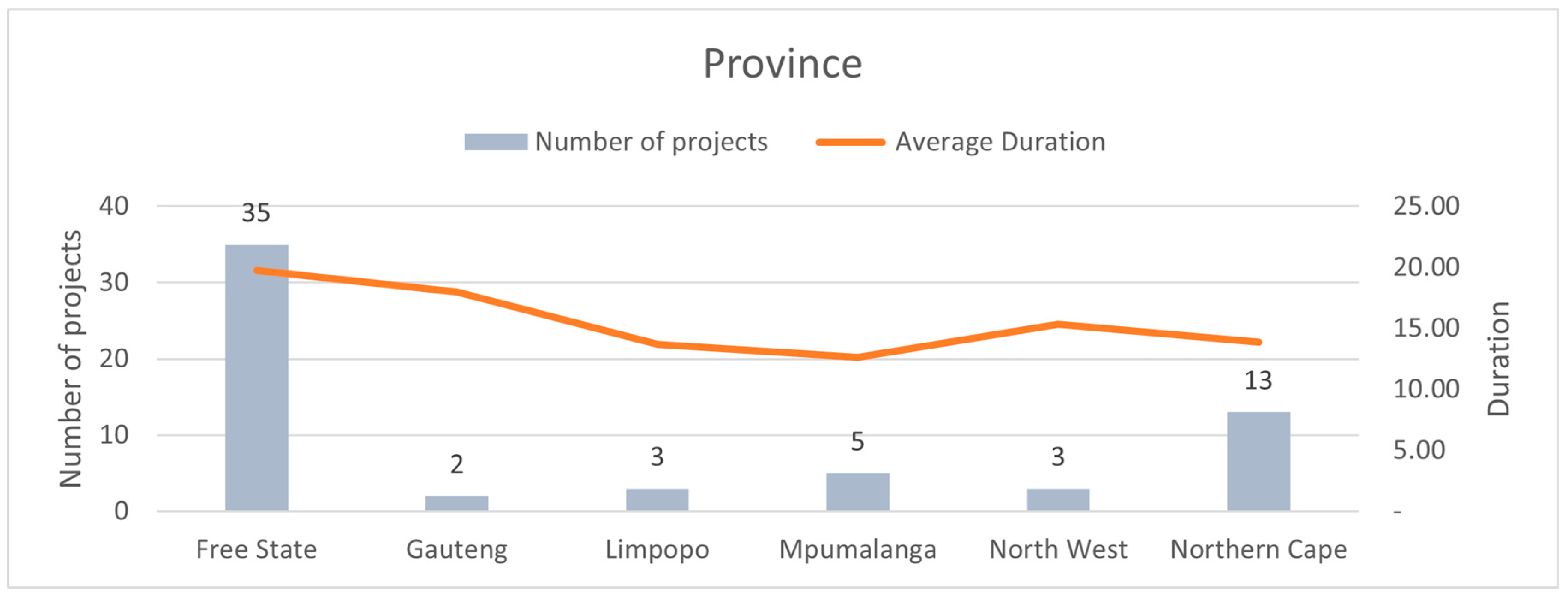
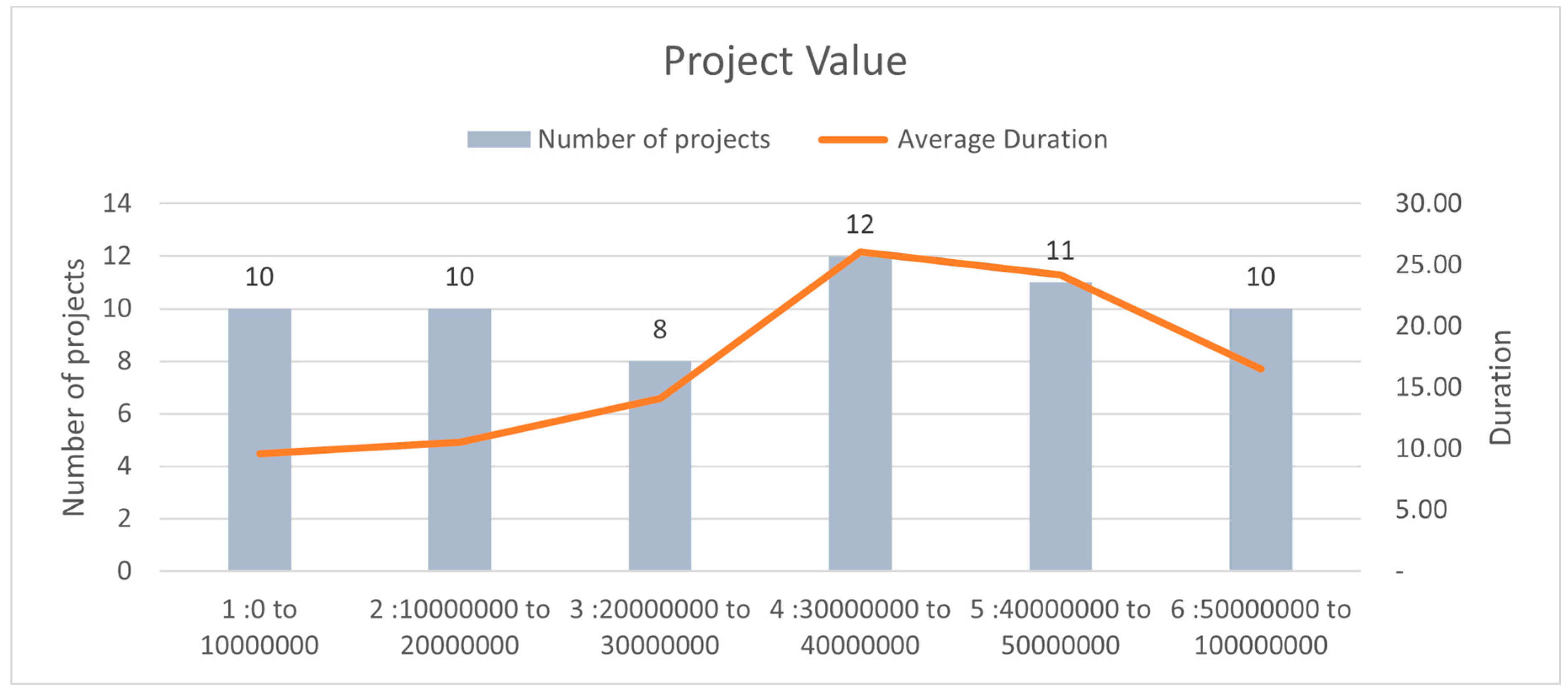
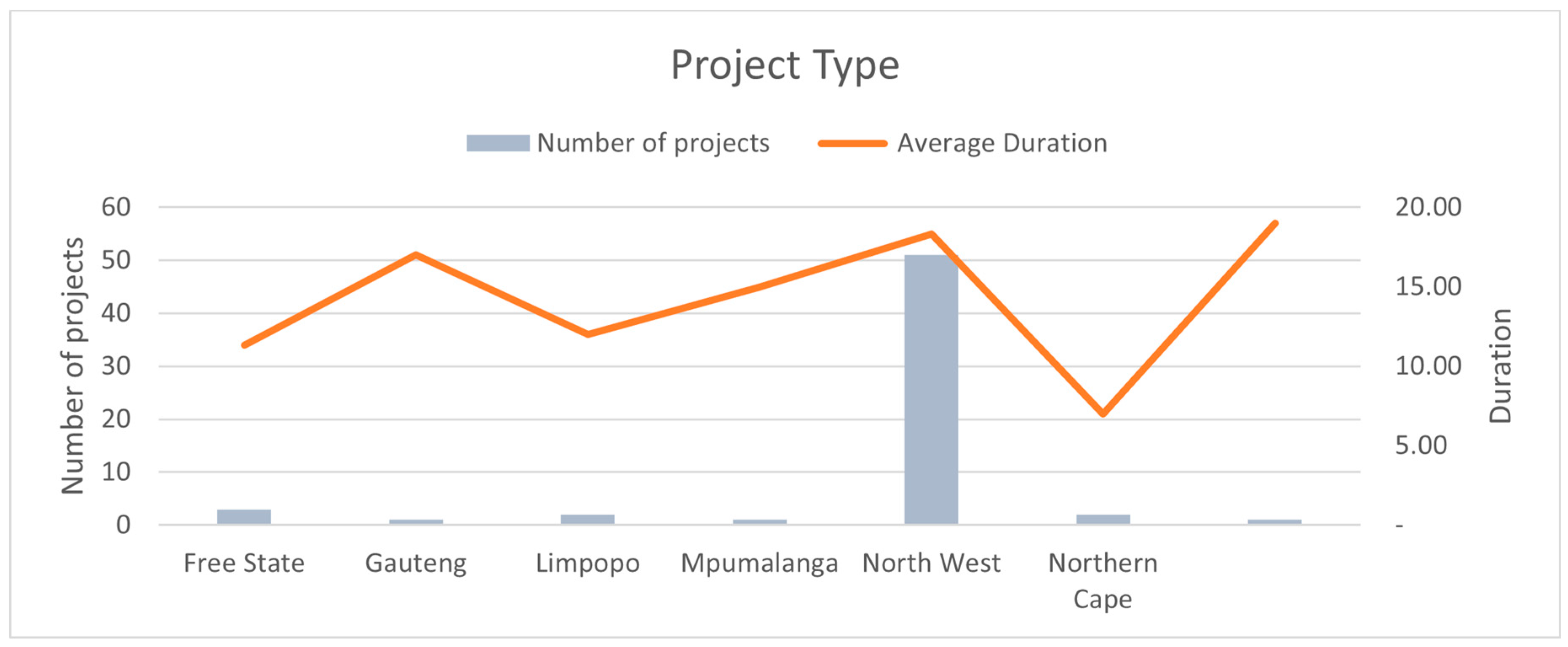
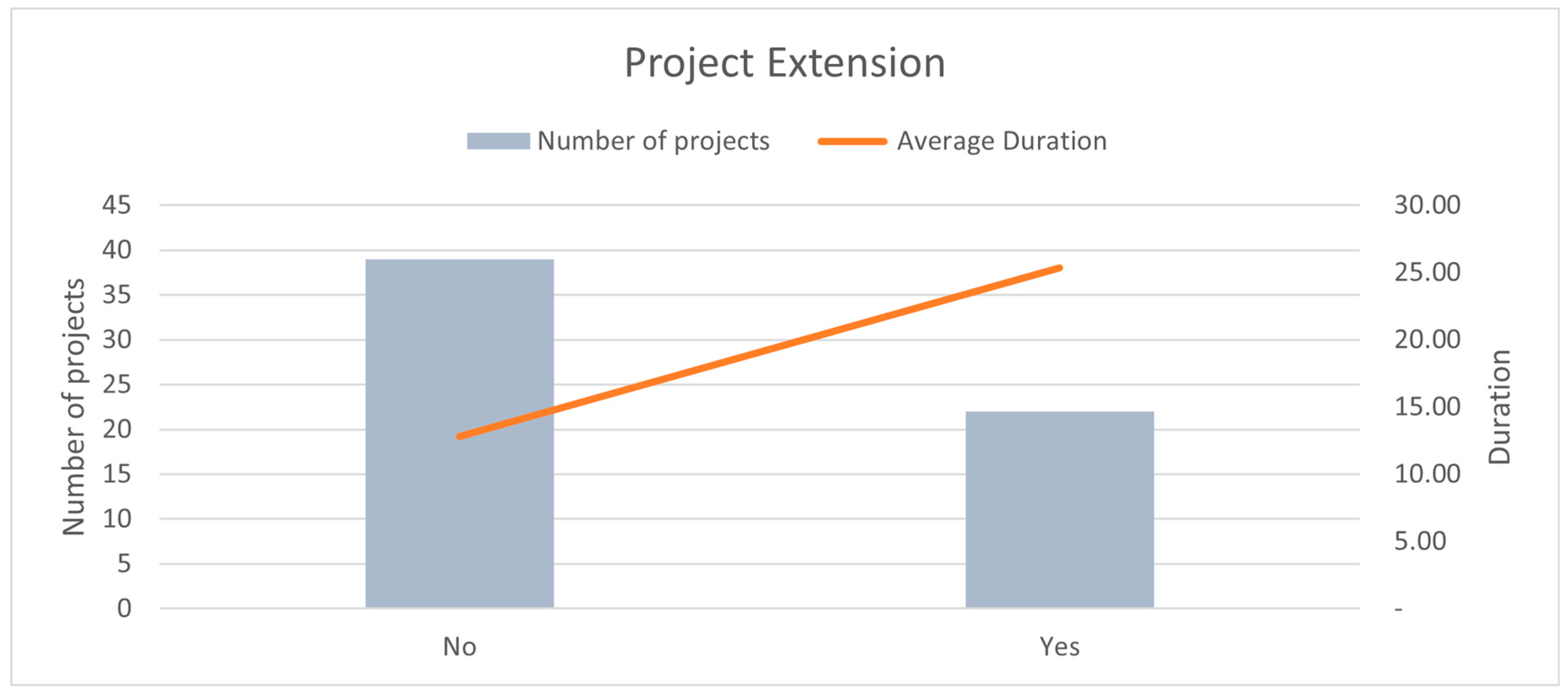
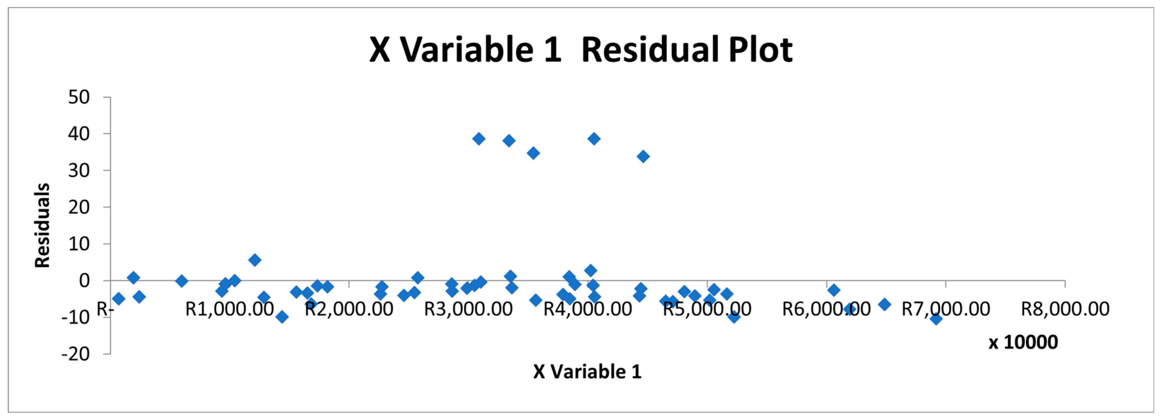

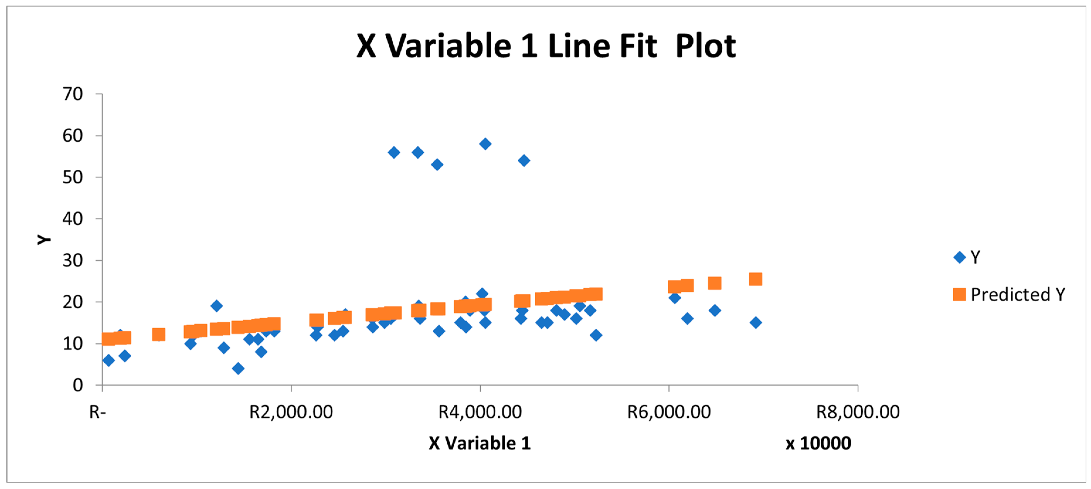
| Regression Statistics | |
| Multiple R | 0.315949 |
| R Square | 0.099824 |
| Adjusted R Square | 0.084566 |
| Standard Error | 11.62519 |
| Observations | 61 |
| ANOVA | |||||
| df | SS | MS | F | Significance F | |
| Regression | 1 | 884.2156 | 884.2156 | 6.542718177 | 1.31% |
| Residual | 59 | 7973.555 | 135.145 | ||
| Total | 60 | 8857.77 |
| Coefficients | Standard Error | t Stat | P-value | Lower 95% | Upper 95% | Lower 95,0% | Upper 95,0% | |
| Intercept | 10.85858 | 2.940175 | 3.693176 | 0.000486005 | 4.975306335 | 16.74186 | 4.975306 | 16.74185974 |
| X Variable 1 | 0.0000% | 8.21E-08 | 2.557874 | 0.013120283 | 4.57323E-08 | 3.74E-07 | 4.57E-08 | 3.74386E-07 |
Disclaimer/Publisher’s Note: The statements, opinions and data contained in all publications are solely those of the individual author(s) and contributor(s) and not of MDPI and/or the editor(s). MDPI and/or the editor(s) disclaim responsibility for any injury to people or property resulting from any ideas, methods, instructions or products referred to in the content. |
© 2024 by the authors. Licensee MDPI, Basel, Switzerland. This article is an open access article distributed under the terms and conditions of the Creative Commons Attribution (CC BY) license (http://creativecommons.org/licenses/by/4.0/).


