Factor-Based Trading Strategy for Index Rebalancing: Predicting Abnormal Returns Using Logistic Classification

Satish Mandavalli

doi:10.20944/preprints202410.0271.v1

Submitted:

02 October 2024

Posted:

04 October 2024

You are already at the latest version

Abstract

In this paper, we present an approach which examines whether there are persistent abnormal returns around the periods of index rebalancing, using a factor-based framework. By employing this methodology, we observe the yield of normal returns around these events, although the detected abnormal returns may not usually be statistically significant. Therefore, we conclude the study by addressing how one such supposed strategy for rebalance trading is systematic constructive by supervision of some predictive model for the candidates based on all available in the TSX universe for inclusion into the S&P Capped TSX Composite Index in about a month. Trade signals were constructed using a logistic binary classifier based on the same factors used by the index committee to determine the qualifications for inclusion in the index. The problem of a very low probability of out of context security selection for addition to the index is solved at the expense of random over-sampling. In the end, these trade signals were then used to create a hypothetical trading strategy that outperformed the back-test period.

Keywords:

Index

;

Predictive Model

;

Returns

;

Yield

Subject:

Computer Science and Mathematics - Artificial Intelligence and Machine Learning

I. Introduction

The use of passive strategies has gained prominence considerably in the period that has elapsed since the global financial crisis. In 2016, passive investors held approximately a third of the world’s equity asset holdings. The cost of passive management is relatively low, as turnover and management of passive portfolios incur minimal research and management costs, which leads people to assume that passive investment does not have any internalized wedge. Including a stock in an index can produce positive excess returns for that stock in the short run, but rather interestingly in the long run, the returns are usually negative [1,2,3,4,5]. Negative abnormal returns are assumed to commence several months before the rebalance takes place and to subside only after the rebalance takes place.Since changes to the index methodology are well advertised in advance and such index changes take place on well-established dates with rules on when and what changes should be made. Nevertheless, there is still a gap in understanding the exact extent and length of these troubling returns in the research papers, especially in the Canadian case. Being able to estimate and pinpoint the extent and duration of such reversions would offer index fund managers a chance to reduce trading costs and improve performance [6,7,8,9,10].

Therefore, the research paper strives to resolve the fundamental question i.e. if a security is added to an index, then at what extent can its returns be directly attributed to its inclusion in that index? If abnormal returns exist, can a portfolio be constructed to exploit this inefficiency? The present study, consistent with the research question outlined above, is structured around three main goals. First, it desires to estimate cumulative abnormal returns ascribed to index events. Following this point, these events bring active reactions in the market. Investors may exploit these abnormal returns around the event to draw immediate returns. Second, the study seeks to employ machine learning techniques, such as random forests, gradient-boosted trees and support vector machines, to identify those securities that are expected to be incorporated in the Composite Index before the pricing of these changes in the market. By predicting other reforms to the index which hasn’t been enacted yet, the model can give investors first advantage when it comes to changes in the market. Finally, the analysis in the transcending section will be applied to expand the scope of investment decisions directed at rebalancing the constructed index.

The study is as follows; similar papers are shown in the following section. The materials and procedures are provided in Section III. The outcomes' pre-implementation is given in Section IV. The post-implementation outcomes are given in Section V, and in Section VI, we wrap up the study with some conclusions and ideas for future work.

II. Related Works

The notion of event study, which is widely used, and to which [11] have contributed, consists of estimating the abnormal returns of security by estimating its returns with the returns predicted by the market model. This approach allows a sharp comparison of returns prior and post an individual event by using the regression model adopted by [12]. [13] were critical of the usual approach of measuring how unusual returns compared to the variance in returns, as they pointed out, quite appropriately, that it leads to the erroneous rejection of the null hypothesis in many instances where the assertion of the event itself is rather volatile. However, this is still possible in the majority, though not all, of the studies where a cross-section analysis would be a better method whereby the induced volatility is very low in some cases and hence simpler significance tests are appropriate. [14] created an alternative method by creating a comparison between discrete returns on a security against the market. [15] refined this framework by estimating the effects of mergers measured in cash flows. The purpose of this approach was to quantify changes in the discount factors over time, pre- and post-merger, although this has limited applicability in assessing returns because of index inclusions. Market capitalization and liquidity accomplish a higher percentage in the S&P/TSX Composite and Sector Indices which is almost unsurpassed. One of the prerequisites that qualify security for inclusion into the S&P/TSX Composite is that the Volume-Weighted Average Price (VWAP) should averagely be greater than a dollar in the past three months and three days of the last month. There is also another requirement concerning the stock as it must also be worth Jamaica at least 0.05% of the index value. The S&P and TSX Sector Indices replicate these inclusions according to GICS sectors. It is important to note that membership in the S&P/TSX 60 which is largely a function of market capitalization and sector balance with the approval of committee members, does not have a fixed schedule. It has been demonstrated by considerable research that the inclusion of the index leads to abnormal returns in the short run and in the United States for instance, this yields a rise in stock prices between 5% and 7% upon inclusion in the S&P 500, 400 or 600 indices. In contrast to this, exclusions are associated with negative returns and in the case of S&P 600 deletions, it is about – 15% returns.

The convergence in stock price ‘cause’ is believed to be the net imbalance of demand for shares, as included demand is generally increased while exclude leads to too much supply. Also, the volatility, in normal circumstances, is anticipated due to the speculative prepositioning that occurs before the official date of index changes. Machine learning applications in finance have generated more interest, especially in trade scheduling problems such as [16]. Market impact model and trade execution optimization have utilized reinforcement learning as discussed by [17]. These models learn trading rules by maximizing profit and minimizing losses. There are still a few gaps that have been left particularly so in the case of Canadian Indices. Such factors are the possibility of an index predictive machine learning, the impact of volatility on index rebalances, and the transaction costs at the fund level which are generally assumed to be derived from the abnormal returns associated with index re-balancing events.

III. Materials and Methods

A. Dataset Analysis

The study contained a substantial amount of work on improving the data structures and workflows for the analysis of large amounts of data in an efficient and scalable manner. At the outset, exploring for Canadian index change data proved relatively of a laborious task. While Wharton Research Data Services (WRDS) databases were being searched, it was noted that the Center for Research in Security Prices (CRSP) dataset has American indices only. Also, while the RavenPack dataset was being searched for insights from PR Newswire or feeds from high profile providers such as DowJones, it was no real benefit in the investigation for index changes. It examines for such changes in other possibilities such as board room changes or shifts in analysts’ ratings. Ultimately, about 10 years’ worth index change data encompassing 5376 changes was sourced from S&P Capital IQ using the Key Developments by Type: Index Constituent Drops OR Index Constituent Adds [All History] and Exchange Country (All Listings): Canadian. Further, information on present index components consisting of 827 names for the entire TSX indices was sought from S&P Capital IQ. Canada ITG furnished also a list of the TSX Composite changes made as from Q1 2012 concerning 208 entries. All providers of Exchange-Traded Funds (ETFs) are obliged to publish a report on the composition and the level of the fund daily and Bloomberg collects such data which is an estimate of the composition of the indices. This information was vital to assess the volume of trades that had to be carried out by fund managers in case a deletion occurred, and the positions were to be closed entirely, and it was also useful for presentations. The market impact could be estimated by looking at the amount of active relative weight in a fund versus the fund’s total net asset value [18,19,20,21,22,23,24].

This paper investigates the relationship between financial and accounting data with changes to be made in the index in the future. The financial data sourced from S&P Capital IQ for the period Q1 2010 to Q4 2018 was append into the predictive rebalancing index models. Nevertheless, the addition of this data did not result in any improvement in the accuracy of the predicted values of the model. Earlier attempts were made to retrieve financial data from The Globe and Mail website using an HTTP GET vulnerability, although this technique was not applied during the later phases. To make the assumptions consistent with the setup of the models, other market and factor data (market returns, risk free returns, SML, HMB, etc) were obtained from Kenneth French’s database. Industry comparatives included in Aswath Damodaran’s database were also used, but these did not enhance forecasts. TSX Composite index volatility data was taken from the Bloomberg system. In the beginning, a Canadian volatility ETF (HUV) was used in the analysis as a proxy; however, that ETF was not effective due to contango and backwardation factors. The price data that was employed spans from daily closing bid prices from Q3 2012 to Q3 2018 disbursed by the Canadian Financial Markets Research Centre (CFMRC). These included intraday trade and quote data which were obtained from the TMX Grapevine platform, although its effectiveness was hampered by technical hitches. An event study was also carried out to measure abnormal returns at the time of index rebalancing events. The first method was based on the three-factor model of the Capital Asset Pricing Model (CAPM). It was then superseded by the five-factor Fama-French model and finally multisector model incorporating market, sector and industry to capture more rigorous complexities of the index inclusion process, especially for large-cap stocks as well. Cumulative Abnormal Returns (CAR) were computed to establish the importance of the apparent patterns [25,26,27].

B. Model Analysis

The focus of the model is on those equities which can be expected to be included in the TSX Composite Index. Upon such securities being identified, the results of the classification will be incorporated into the portfolio construction script whereby, the trade signals will then be backtested with historical returns. This end-to-end process will be pursued so that the outcomes are not only implementable but also explainable, thus limiting further risks and adding value to more studies. Several parameters will be used in the selection process. First, to determine how well the model can classify the data, the area under the Receiver-Operator Characteristic (ROC) curve will be evaluated. Within predictive modelling, this is a requisite parameter and more so regarding the classification measures of the model. The model's success hinges on balancing false negatives and false positives, while ensuring profitable returns when back-tested against historical data to achieve the investment strategy objective. Only a small number of securities are added to or removed from the TSX Composite index each month, leading to a significant class imbalance in predictions. To address this, random-sampling techniques were employed using the sk-learn Python library. A market capitalization cutoff was implemented, excluding securities with a market cap exceeding 0.6% of the index’s total value, to improve accuracy in predictions. Some machine learning techniques, such as random forests and gradient boosted trees, can handle this problem well since they respond in a non-linear manner. Furthermore, a technique called Synthetic Minority Over-sampling Technique (SMOTE) created a training set with additional interpolated data points. Such a method, which has been incorporated within the framework of SMOTE, augments the dataset with observations well unlike the existing ones which are plausible in the dataset used for training. Unfortunately, SMOTE reduced performance on the test set since new outliers were introduced in between securities about to be included and ones that large caps for domicile rules. Rather than having two separate clusters within the training set, a low cap security that can be qualified and a high one that cannot be qualified, SMOTE, which took the place of both expanded the training’s over wealth of the data rather than too realistic points eroded the model’s effectiveness. To defend against overfitting, the sample set was randomly assigned into two distinct groups: a training set that constituted 80% of the population and a test set that constituted the remaining 20% of the population. In this case, the model is built on the training dataset, and its evaluation is performed on the test dataset. Finally, the model was validated using the test set to assess the algorithm in real-time conditions.

To enhance the model training process, the characteristics used by S&P to classify securities for Composite index inclusion were integrated into the training dataset. These included features such as float turnover, share of the index's market value, VWAP, volume, and market cap. The features were estimated every month according to S&P standards and were employed for the assessment of the securities in question. The most typical models used random forests, gradient-boosted trees, and logistic regression for the binary task of classification. Although some pursuit of artificial neural networks was entertained at quite an early stage, they were rejected as being out of the scope of the undertaking. To employ the learnt binary classifier, a custom signal generation script was created. This script generated a list of securities likely to be included in the Composite index, mapping trades to specific dates. In the case of probabilistic models, such as logistic regression, trade weight in the portfolio was determined by the averaged predicted probability of the signal. In case the model returned outcomes in terms of 1 and 0 only, in the case with support vector machines, all trades were equally weighted. This stand-alone script lets various signal generation techniques and portfolio construction methods be tested independently.

IV. Pre-Implementations

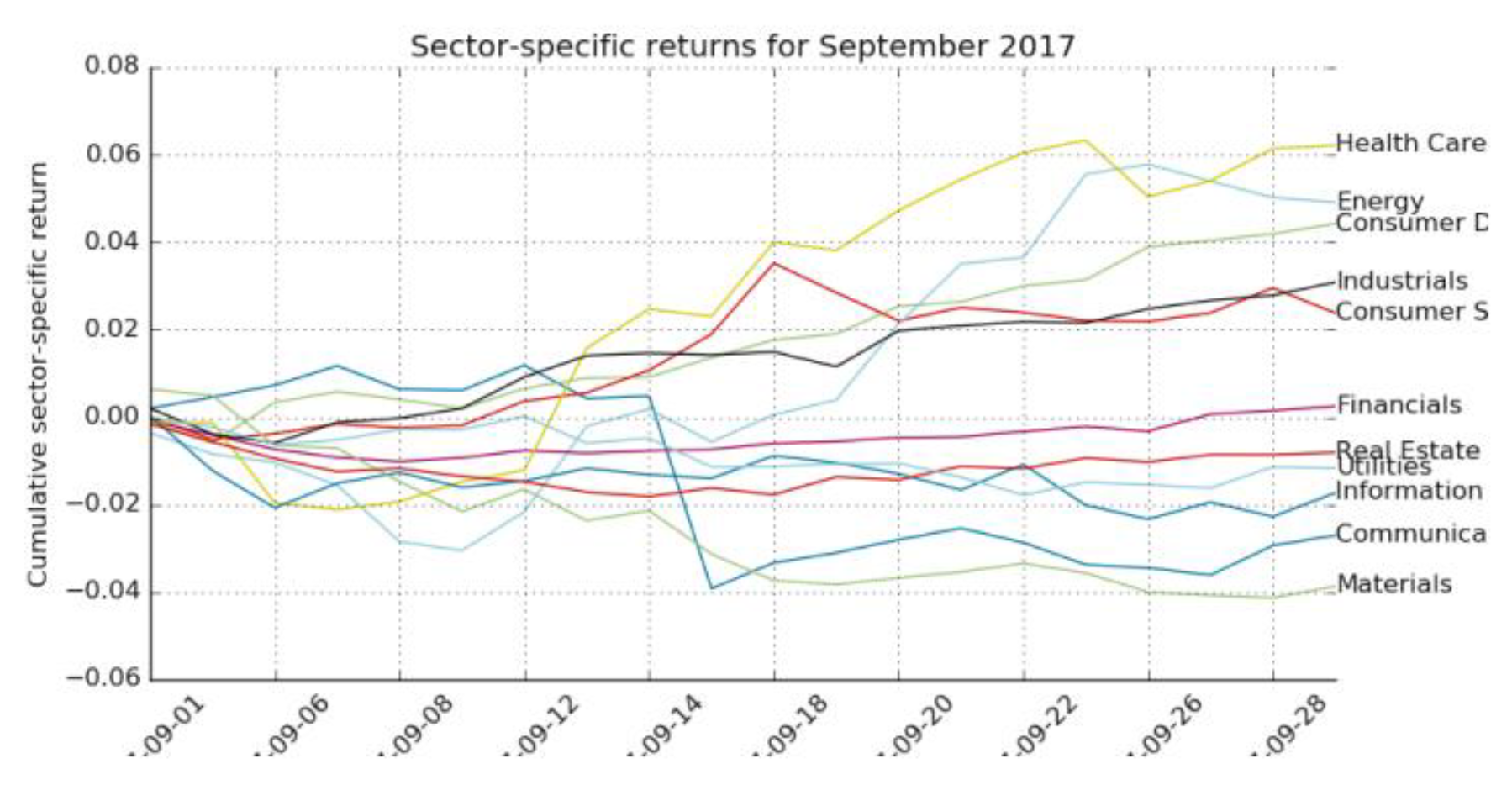
A factor model was forgone before any abnormal returns could be calculated: a factor model was constructed as described in the Figure 1. The daily–mean returns on market and Global Industry Classification Standard (GICS) sectors and industries were calculated on an Equal weight basis. The exposition offers information for each GICS industry category rather than the country category. These daily returns were also estimated for the individual GICS industries. Daily sector and industry return together with daily market returns were used to calculate coefficients for each security through linear regression analysis. This method helps assess how individual securities react to fluctuations in the market, estimating their performance in the composite of the market. Example coefficients for companies regulated in TSX belonging to the “Copper” GICS industry code are illustrated in Table 1.

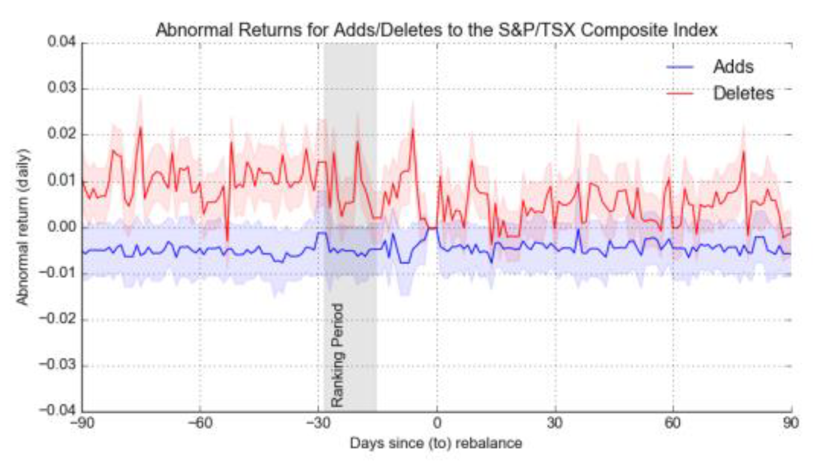
Thus, instead of making clusters or peers for every security, these were created more easily. In this way, those factors serve to calculate the expected return per security for comparison with what was obtained in practice. Applying the existing factor model, the estimated the expected return for each treated security about other market competitors and their respective sectors over the test period. As these expected returns are compared with the daily security returns of each security, the calculation of the abnormal returns, which are shown in Figure 2. It can be assumed that over the course of the whole observation period, the accumulated fault concerning the addition of securities continues to be negative in nature with only a minor increase around the rebalancing day. Throughout the study period, the dispersion of the daily returns of securities retained the same trend, which suggests that the rebalancing itself does not cause any additional volatility.

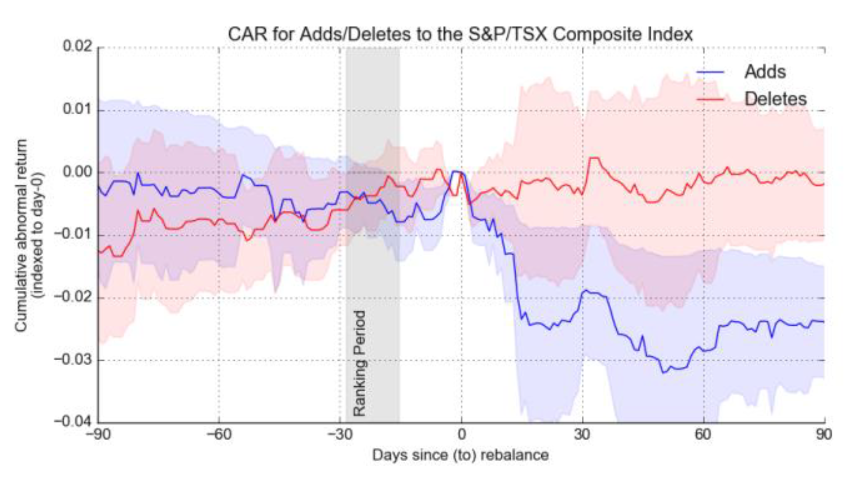
While incorporating triggered volatility makes the use of our simple test statistic - cummulative abnormal return to return variance is reasonable as shown in Figure 3. Once daily abnormal returns are computed, their representation on a graph readily facilitates the construction of cumulative abnormal returns within the confines of the portfolio’s framework. A noteworthy observation can be discerned from the paired graph; typical returns interestingly rise sharply towards the introduction of new stocks to the composite index. This tendency suggests that market investors buy certain stocks even before the announced adjustments increase their prices because these stocks are expected to be included in the next index rebalance.

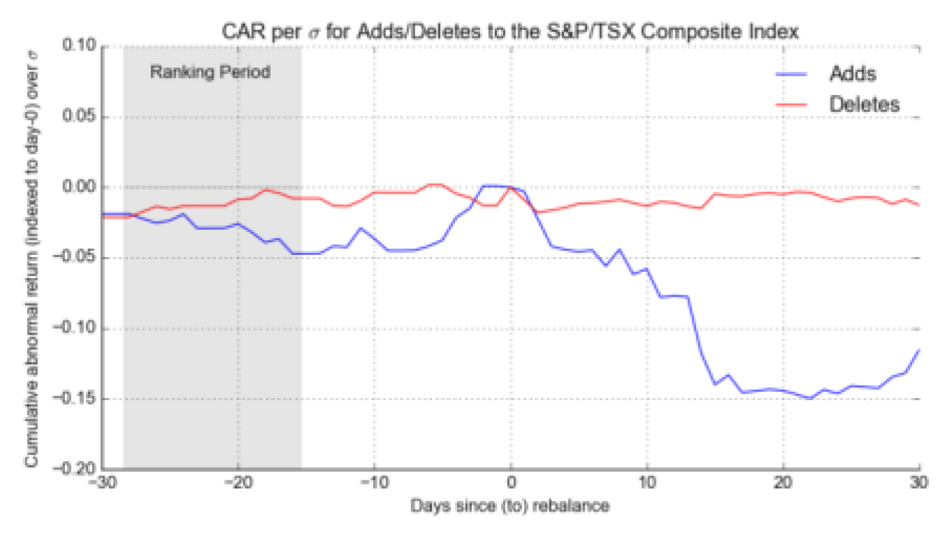
Although the returns are high initially, this situation does not always persist. After the index adjustment, any gains made during trading are often reversed and even fall below those in most cases as shown in Figure 4. This is explained by the investors' behaviour of "buy the rumour and sell the news" whereby they buy shares in anticipation of an index enhancement and then get rid of them on the actual event. Therefore, it is very important to comprehend how this situation takes place in coming up with an effective trading strategy. Because of such behaviour, investors capable to determine the right timing for entering or exiting a position in the market with the anticipation of getting the desired investment returns while managing risk. Further, the significance ratio calculation will not be very hard. As for the portfolio of indexes after the rebalance period was 4 Thursdays after the update, on average 2-week cut back in active returns yields -15% daily returns 20 days post-rebalance. It suggests that the cumulative abnormal returns remain below the daily returns, within their standard deviation. Without resorting to a higher level of precision in examining statistical significance, such abnormal returns generate in response to index rebalances. For this reason, these more qualitative results should be subject to more complex econometric analysis for unification of these findings.

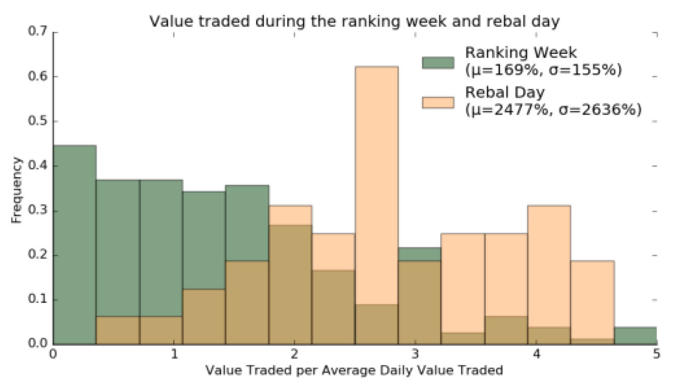
These anomalous returns also come with volume surprises as shown in Figure 5. While it has been determined that trading volumes in the period of the interval period are with the average, it has been shown in the graph that the volume on the days of the rebalance is generally much higher. Interestingly, on rebalance days, the volumes are about 2477% of the average daily volume. Few trading days create an outlier with very high-volume surprises and therefore cause skewness. In normal cases, volume on rebalance days is owned 2-4 times ADV volume.

V. Post-Implementations

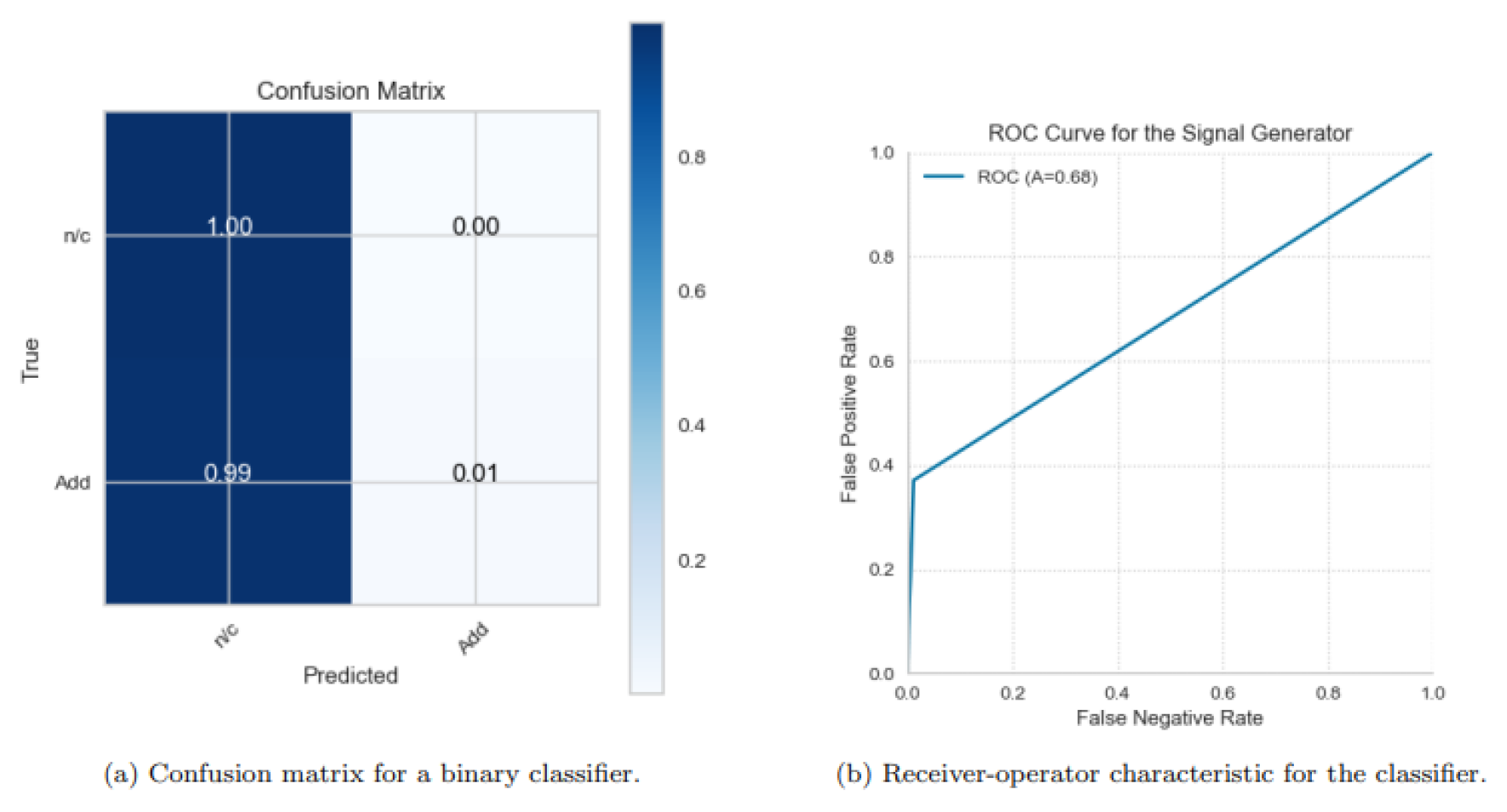
Since volume weighted market cap is about the percentage contribution of a security to the index market, it is evident that due to the correlations between some of the factors which are, percentage holdings and others, there are two main factors which are orthogonal to each other and which form bases for the rest of the features. These are turnover and market capitalisation contribution, whose distributions in other words the distribution of security months which preceded preventing an addition and which preceded non-change again. The examination makes it possible to gather the most essential understanding of the attributes that certain classification techniques will be able to seek out. Since newly added securities have a higher premium than the index, they also turn in more float than what is proportionate to the index. This indicates that instead of market capitalisation, liquidity might be a more reliable factor in forecasting so-called changes in index status. The results indicate that factors other than those identified as used by the ranking committee in most instances hold predictive potential. Having formed the Composite index, it was necessary to classify the dataset and recommend several binary classifier algorithms to facilitate the addition of securities. The evaluation of the model relied on maximizing both true positives and true negatives classification performance, addressing the class imbalance within the sample. While the random forest classifier style is currently trending, it generally performed unsatisfactorily with respect to test data, often resulting in a high false negative rate as shown in Figure 6. The confusion matrix indicates that the addition of index changes was frequently misclassified as no change. This trend is further reflected in the ROC curve, which shows that even when a low false negative rate is maintained, the model still produces a significant number of false positives. Ultimately, the model trained itself to predict a status quo outcome, thereby limiting its effectiveness in identifying actual changes in index composition.

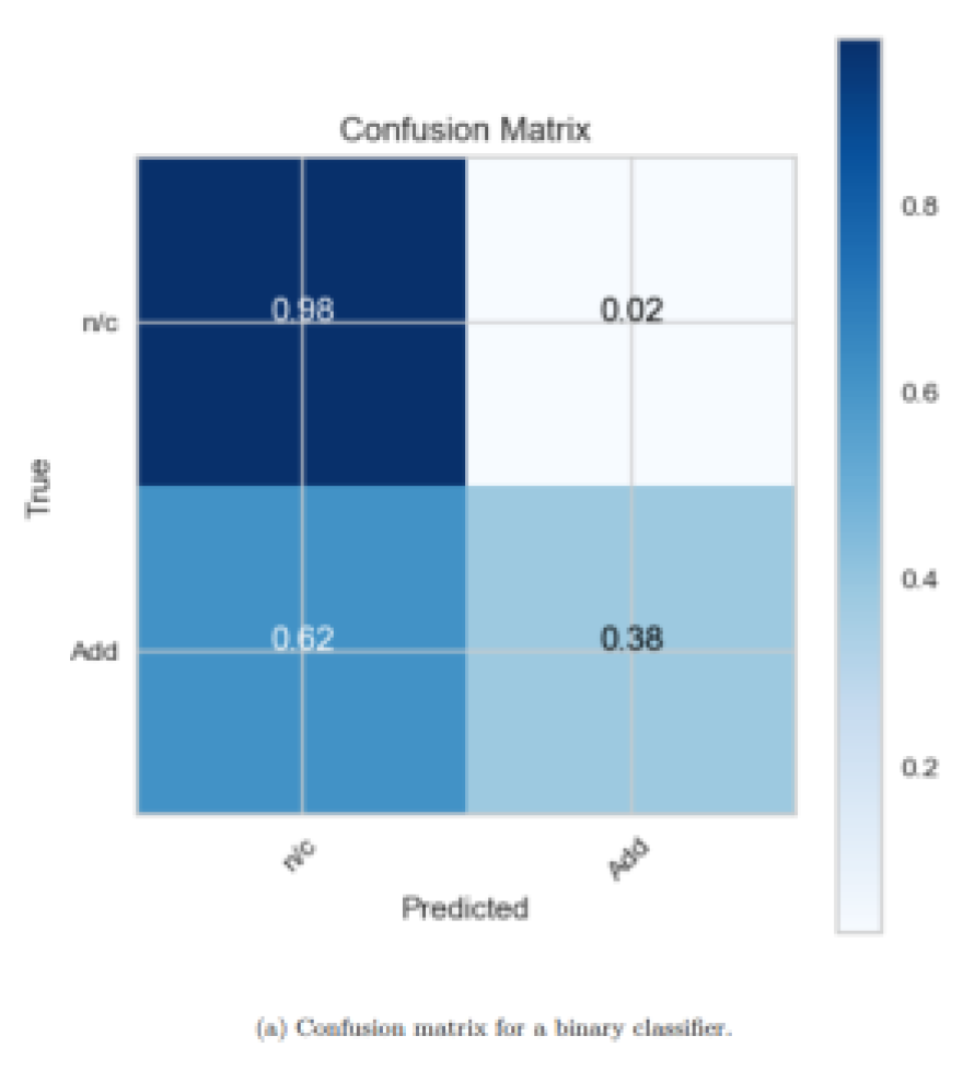
The contributors behind the classifiers' choice in the model are mainly focused on two things which include the inequality in contribution to the index market capitalisation and the liquidity characteristic regarding the support vector machines as shown in Figure 7. However, this model perform ably beat the random forest algorithm; however, their reports on false negatives were still high at 62%. This suggests that even if the support vector machines can perform well in classifying data into different classes, they do not appear to be prosperous in classifying classes which include the securities that should most effectively modify the index. It may assist in increasing the optimization of hyperparameters or adding new dimensions that would affect the trading volume and volatility to enhance the prediction accuracy and reduce possible errors. Furthermore, additional improvements in the robustness of the model's understanding of market forces can be achieved through ensemble techniques that employ several distinct classifiers. In this way, it is possible to come up with a diagnosis and treatment that is desirable and right to achieve the set goals of the SDC, that is, efficient and effective management of the Composite index. This progressive refinement is vital in responding to the need to improve the financial markets and maintain the model's stability over time.

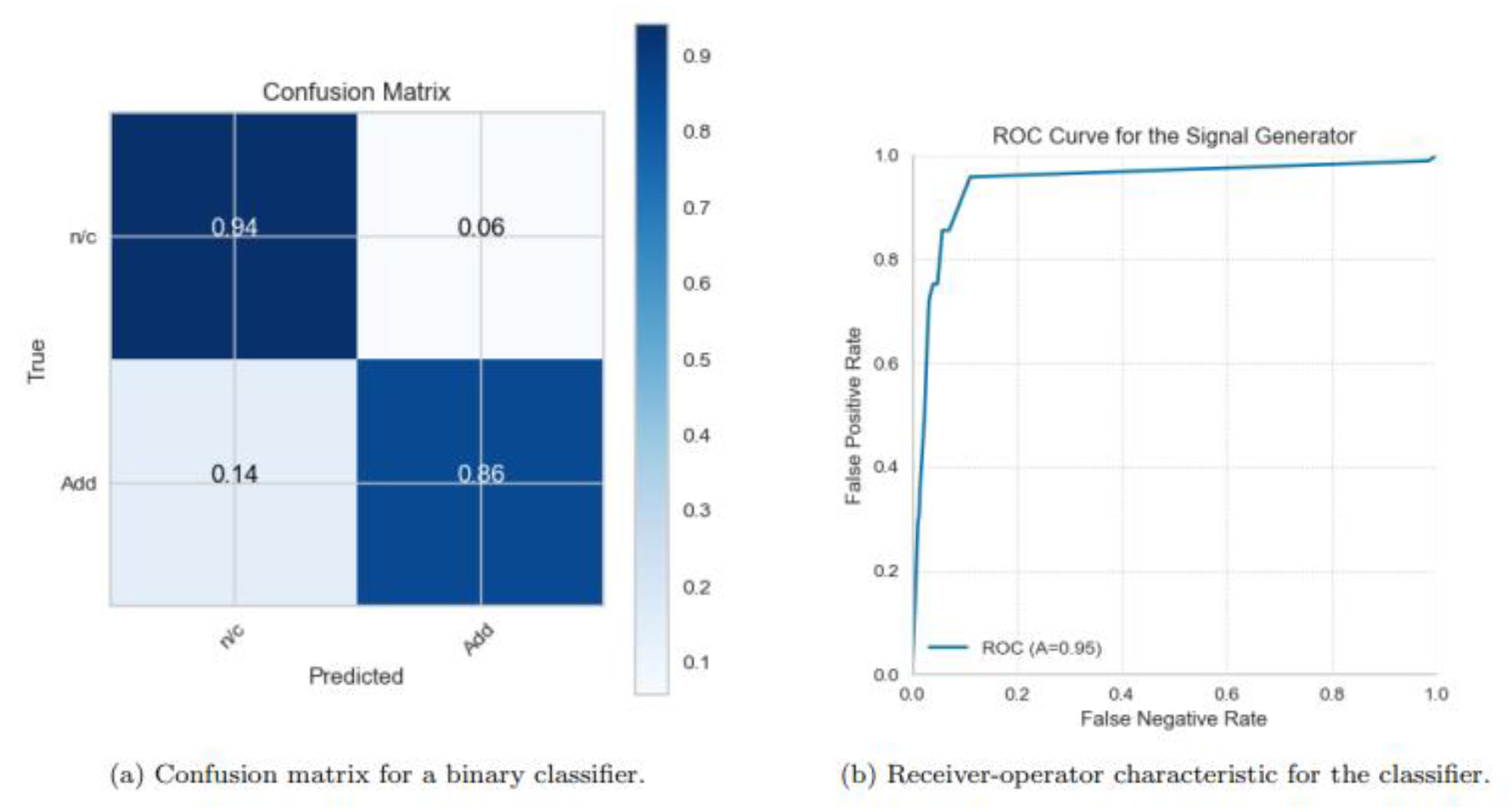
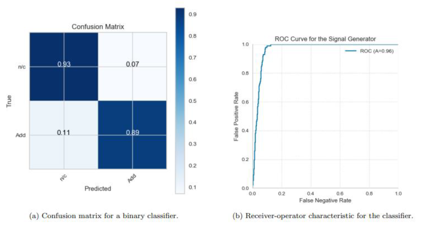
On the other hand, the gradient-boosted tree model improved on the previous angle in the sense that it does not create too much bias and overfitting, yielding an area under the ROC curve of 0.95, while a false negative rate of 14% was present as shown in Figure 8. Surprisingly, the logistic regression binary classifier, despite being the simplest model examined, exceeded the performance of the others as shown in Figure 9. Its false positive rate was marginally higher than that of the gradient boosted tree (7% against 6%), but it showcased a markedly improved false negative rate (11% versus 14%) and a better area under the ROC curve (96% compared to 95%). The sharpness of the ROC curve suggests that a nearly zero false positive rate could be achieved with just a slight increase in false negatives.

VI. Conclusion and Future Works

This study describes a methodology designed to identify places where investors earned abnormal returns in the event of index rebalancing, noting that abnormal returns do exist, however, the validity of them appearing statistically is rather doubtful. The study this time goes a step further and proposes a trading strategy that forecasts which securities within the TSX are most likely to be added to the Composite index. This prediction employs, among other tools, a logistic binary classifier using the factors employed by the S&P Dow Jones index committee for inclusion criteria during the construction of the indexes. Random over-sampling techniques were employed to deal with the problem of very low random chances of inclusion of some arbitrary security in an index. The signals generated from such models were used to create an experimentally constrained successful investment portfolio, thereby indicating the practical possibility of exploiting the inefficiencies of the market regarding index rebalancing. However, the study recognizes several limitations necessitating future research. These include the potentially overly complicated hedging strategy, the omission of deletions, the restricted number of generated signals, and the risk of missing additional returns by postponing trades until the conclusion of the ranking window. Addressing these limitations could enhance the strategy's robustness and economic feasibility. Collaboration opportunities for testing and assessing these signals were also contemplated, although not pursued at this stage.

References

V. Kanaparthi, “Exploring the Impact of Blockchain, AI, and ML on Financial Accounting Efficiency and Transformation,” Jan. 2024, Accessed: Feb. 04, 2024. [Online]. Available: https://arxiv.org/abs/2401.15715v1.
Kanaparthi, V. Examining Natural Language Processing Techniques in the Education and Healthcare Fields. Int. J. Eng. Adv. Technol. 2022, 12, 8–18. [Google Scholar] [CrossRef]
Kanaparthi, V.K. Examining the Plausible Applications of Artificial Intelligence & Machine Learning in Accounts Payable Improvement. FinTech 2023, 2, 461–474. [Google Scholar] [CrossRef]
Kanaparthi, V. Transformational application of Artificial Intelligence and Machine learning in Financial Technologies and Financial services: A bibliometric review. J. Bus. Res. 2024. [Google Scholar] [CrossRef]
Kanaparthi, V.K. Navigating Uncertainty: Enhancing Markowitz Asset Allocation Strategies through Out-of-Sample Analysis. FinTech 2024, 3, 151–172. [Google Scholar] [CrossRef]
G. S. Kashyap et al., “Revolutionizing Agriculture: A Comprehensive Review of Artificial Intelligence Techniques in Farming,” Feb. 2024. [CrossRef]
Kanojia, M.; Kamani, P.; Kashyap, G.S.; Naz, S.; Wazir, S.; Chauhan, A. Alternative agriculture land-use transformation pathways by partial-equilibrium agricultural sector model: a mathematical approach. Int. J. Inf. Technol. 2024, 1–20. [Google Scholar] [CrossRef]
H. Habib, G. S. H. Habib, G. S. Kashyap, N. Tabassum, and T. Nafis, “Stock Price Prediction Using Artificial Intelligence Based on LSTM– Deep Learning Model,” in Artificial Intelligence & Blockchain in Cyber Physical Systems: Technologies & Applications, CRC Press, 2023, pp. 93–99. [CrossRef]
P. Kaur, G. S. P. Kaur, G. S. Kashyap, A. Kumar, M. T. Nafis, S. Kumar, and V. Shokeen, “From Text to Transformation: A Comprehensive Review of Large Language Models’ Versatility,” Feb. 2024, Accessed: Mar. 21, 2024. [Online]. Available: https://arxiv.org/abs/2402.16142v1.
Marwah, N.; Singh, V.K.; Kashyap, G.S.; Wazir, S. An analysis of the robustness of UAV agriculture field coverage using multi-agent reinforcement learning. Int. J. Inf. Technol. 2023, 15, 2317–2327. [Google Scholar] [CrossRef]
Henrique, B.M.; Sobreiro, V.A.; Kimura, H. Stock price prediction using support vector regression on daily and up to the minute prices. J. Finance Data Sci. 2018, 4, 183–201. [Google Scholar] [CrossRef]
Palomino, F.; Renneboog, L.; Zhang, C. Information salience, investor sentiment, and stock returns: The case of British soccer betting. J. Corp. Finance 2009, 15, 368–387. [Google Scholar] [CrossRef]
Kan, R.; Zhou, G. Optimal Portfolio Choice with Parameter Uncertainty. J. Financial Quant. Anal. 2007, 42, 621–656. [Google Scholar] [CrossRef]
Glosten, L.R.; Jagannathan, R.; Runkle, D.E. On the Relation between the Expected Value and the Volatility of the Nominal Excess Return on Stocks. J. Finance 1993, 48, 1779–1801. [Google Scholar] [CrossRef]
Hansen, P.R.; Lunde, A. A forecast comparison of volatility models: does anything beat a GARCH(1,1)? J. Appl. Econ. 2005, 20, 873–889. [Google Scholar] [CrossRef]
Agarwal, S.; Muppalaneni, N.B. Portfolio optimization in stocks using mean–variance optimization and the efficient frontier. Int. J. Inf. Technol. 2022, 14, 2917–2926. [Google Scholar] [CrossRef]
Kolm, P.N.; Tütüncü, R.; Fabozzi, F.J. 60 Years of portfolio optimization: Practical challenges and current trends. Eur. J. Oper. Res. 2014, 234, 356–371. [Google Scholar] [CrossRef]
Naz, S.; Kashyap, G.S. Enhancing the predictive capability of a mathematical model for pseudomonas aeruginosa through artificial neural networks. Int. J. Inf. Technol. 2024, 16, 2025–2034. [Google Scholar] [CrossRef]
Alharbi, F.; Kashyap, G.S.; Allehyani, B.A. Automated Ruleset Generation for ‘HTTPS Everywhere’: Challenges, Implementation, and Insights. Int. J. Inf. Secur. Priv. 2024, 18, 1–14. [Google Scholar] [CrossRef]
G. S. Kashyap, A. G. S. Kashyap, A. Siddiqui, R. Siddiqui, K. Malik, S. Wazir, and A. E. I. Brownlee, “Prediction of Suicidal Risk Using Machine Learning Models,” Dec. 25, 2021. Accessed: Feb. 04, 2024. [Online]. Available: https://papers.ssrn.com/abstract=4709789.
S. Wazir, G. S. S. Wazir, G. S. Kashyap, K. Malik, and A. E. I. Brownlee, “Predicting the Infection Level of COVID-19 Virus Using Normal Distribution-Based Approximation Model and PSO,” Springer, Cham, 2023, pp. 75–91. [CrossRef]
Kashyap, G.S.; Malik, K.; Wazir, S.; Khan, R. Using Machine Learning to Quantify the Multimedia Risk Due to Fuzzing. Multimedia Tools Appl. 2021, 81, 36685–36698. [Google Scholar] [CrossRef]
S. Wazir, G. S. S. Wazir, G. S. Kashyap, and P. Saxena, “MLOps: A Review,” Aug. 2023, Accessed: Sep. 16, 2023. [Online]. Available: https://arxiv.org/abs/2308.10908v1.
Alharbi, F.; Kashyap, G.S. Empowering Network Security through Advanced Analysis of Malware Samples: Leveraging System Metrics and Network Log Data for Informed Decision-Making. Int. J. Networked Distrib. Comput. 2024, 1–15. [Google Scholar] [CrossRef]
Kanaparthi, V. Robustness Evaluation of LSTM-based Deep Learning Models for Bitcoin Price Prediction in the Presence of Random Disturbances. Regul. Issue 2024, 12, 14–23. [Google Scholar] [CrossRef]
Kanaparthi, V. Credit Risk Prediction using Ensemble Machine Learning Algorithms. in 6th International Conference on Inventive Computation Technologies, ICICT 2023 - Proceedings, Institute of Electrical and Electronics Engineers Inc., 2023, pp. 41–47. [CrossRef]
Kanaparthi, V. The Role of Machine Learning in Predicting and Understanding Inflation Dynamics: Insights from the COVID-19 Pandemic. in 2024 3rd International Conference on Artificial Intelligence for Internet of Things, AIIoT 2024, Institute of Electrical and Electronics Engineers Inc., 2024. [CrossRef]

Figure 1. Cumulative total returns by sector for September 2017.

Figure 2. A portfolio of stocks that is being added to or withdrawn from the S&P TSX Composite Index with abnormal returns.

Figure 3. The S&P TSX Composite Index's cumulative anomalous returns on a portfolio of stocks that are added or withdrawn.

Figure 4. Cumulative anomalous returns over the mean standard deviation of returns for the test period for a portfolio of stocks added to or removed from the S&P TSX Composite Index.

Figure 5. Average value exchanged over the specified timeframe compared to the ADV for all periods.

Figure 6. Performance metrics for a random forest trained using a dataset that was randomly oversampled.

Figure 7. Performance metrics for a binary classifier trained on the randomly oversampled dataset using support vector machines.

Figure 8. Results for a gradient boosted tree classifier trained on the dataset with random oversampling.

Figure 9. Results for a logistic regression classifier trained on the dataset with random oversampling.

Table 1. Coefficients Pertaining to Names Within the Gics "Copper" Sector.

Ticker	Market Return	Sector Return	Ticker Industry	Return Residual
ERO	0.42	0.06	0.03	-0.00
FM	-0.24	0.37	0.17	-0.01
LUN	-0.42	0.26	0.10	-0.01
NSU	-0.15	0.26	0.09	-0.01
TKO	0.06	0.42	0.11	-0.01

Disclaimer/Publisher’s Note: The statements, opinions and data contained in all publications are solely those of the individual author(s) and contributor(s) and not of MDPI and/or the editor(s). MDPI and/or the editor(s) disclaim responsibility for any injury to people or property resulting from any ideas, methods, instructions or products referred to in the content.

© 2024 by the author. Licensee MDPI, Basel, Switzerland. This article is an open access article distributed under the terms and conditions of the Creative Commons Attribution (CC BY) license (https://creativecommons.org/licenses/by/4.0/).

Copyright: This open access article is published under a Creative Commons CC BY 4.0 license, which permit the free download, distribution, and reuse, provided that the author and preprint are cited in any reuse.