High-Energy Neutrino Flavor State Transition Probabilities

Preprint

Article

High-Energy Neutrino Flavor State Transition Probabilities

Altmetrics

Downloads

Views

Comments

A peer-reviewed article of this preprint also exists.

This version is not peer-reviewed

Submitted:

02 October 2024

Posted:

04 October 2024

You are already at the latest version

Alerts

Abstract

We analytically determine neutrino transitional probabilities and abundance ratios at various distances from the source of creation in several astrophysical contexts, including the Sun, supernovae and cosmic rays. In doing so, we determine the probability of a higher-order transition state from $\nu_\tau\rightarrow\nu_\lambda$, where $\nu_\lambda$ represents a more massive generation than Standard Model neutrinos. We first calculate an approximate cross-section for high-energy neutrinos which allows us to formulate comparisons for the oscillation distances of solar, supernova and higher-energy cosmic ray neutrinos. The flavor distributions of the resulting neutrino populations from each source detected at Earth are then compared via fractional density charts.

Keywords:

Subject: Physical Sciences - Theoretical Physics

1. Introduction

As neutrinos oscillate along their path, their quantum mechanical wave packets develop phase shifts that change how they combine to produce a superposition of the three flavors

ν_{e}

ν_{μ}

and

ν_{τ}

. Thus, what starts as an electron neutrino may be detected in a detector as a muon or tau neutrino. On Earth, the electron neutrino,

ν_{e}

, is the most often detected. This makes sense as this state is what we would generally expect from Solar neutrinos [1].

Let us first recognize that the flavor states can accommodate an ultra-relativistic left-handed neutrino. We then allow this neutrino to have a flavor

α (α = e, μ, τ)

and assume the neutrino to have a 4-momentum

P^{μ}

with spatial component,

\vec{p}

. Following [2], we write flavor states of the newly created neutrino

ν_{α} = Σ_{k} U_{α k}^{*} ν_{k},

(1)

where

U_{α k}

is a unitary mixing matrix.

According to Giunti and Kim [2], observations go on to show that when considering that our acquired state,

ν_{k}

, is a massive neutrino state, with its momentum

\vec{p}

as an eigenstate of the vacuum Hamiltonian,

H_{0}

. This can be written as

H_{0} ν_{k} = E_{k} ν_{k}

(2)

where,

E_{k} = \sqrt{{\vec{p}}^{2} + m_{k}^{2}}

The total Hamiltonian in matter can then be written as

H = H_{0} + H_{1}

(3)

where

H_{1} ν_{α} = V_{α} ν_{α}

[2]. This tells us then that our effective potential from our initial neutrino,

ν_{α}

, is then described by the component,

V_{α}

[2]. We have seen that propagation of neutrinos is of quantum mechanical interest due to the phenomenon of state mixing; the production of neutrinos, on the other hand, garners appeal due to its implications for astrophysical environments.

As the interior of a celestial body generates its own magnetic field via currents generated by its rotation, the inner magnetic field has a significant effect on charged particles on the outer surface of the body. When considering a star’s collapse, we must insist on the acceleration of the protons and electrons within the core of the collapsing star. This acceleration is primarily caused by the amount of pressure building up during the infall phases of the collapse. A property of a planet’s magnetosphere is that it has the ability to block cosmic radiation. However, as of recent observations, cosmic rays may also aid in the acceleration of particles from within the core [3]. In this work, we analyze the possibility of neutrino generation from such cosmic rays.

Several factors must go into the description of the acceleration of particles within a magnetosphere. This study looks at a couple of those factors, namely the observation and study of distant cosmic rays and the first-order and the second-order Fermi acceleration. Fermi acceleration is a process of by which a charged particle gains energy due to the shock speed or moving magnetic mirrors, with the order simply referring to the scaling of the energy gained with velocity. During the first-order process, the acceleration is expedited by magnetic variations within shock waves. We can observe the first-order Fermi acceleration case when a star collapses in on itself, primarily during the bounce phase. Right before the material bounces back after collapsing inward, a shock wave is produced. This aids in the acceleration of charged particles within the magnetosphere itself [4]. Supernova remnant shocks are an important astrophysical setting for first-order Fermi acceleration (diffusive shock acceleration), and are considered here as a site of neutrino production [3].

During second-order Fermi acceleration, stochastic acceleration by magnetic mirrors will have a role in answering each of our questions as well as playing a major part in the solution with regard to the probability of a complete flavor transformation. Magnetic mirrors assume the role of bouncing a particle back and forth accelerating it outward. The magnetic mirrors are in the form of a magnetic cloud pushing the charged particles along [4].

2. Neutrino Cross-Sections

Since the first direct neutrino detection by Frederick Reines and Clyde Cowan in 1956, neutrino cross sections have been notoriously small, with individual interaction cross sections estimated to range from

σ \equiv σ_{ν_{μ} - e \to μ - ν_{e}} \sim 1.33 \times 10^{- 38}

{cm}^{2}

\sim 2.67 \times 10^{- 38}

{cm}^{2}

[5].

The simplest method for calculating cross sections is by finding that

\frac{d N_{r}}{d t} = σ_{r} \cdot \frac{d N_{f}}{d t} \cdot n_{b} \cdot d

(4)

where,

n_{b} \cdot d

is the number of targets per surface unit with d being the individual target width. Here,

N_{f}

describes the number of particles within a beam [6]. After integrating over t, we find

σ_{r} = \frac{N_{r}}{N_{f}} \frac{1}{n_{b} \cdot d}

(5)

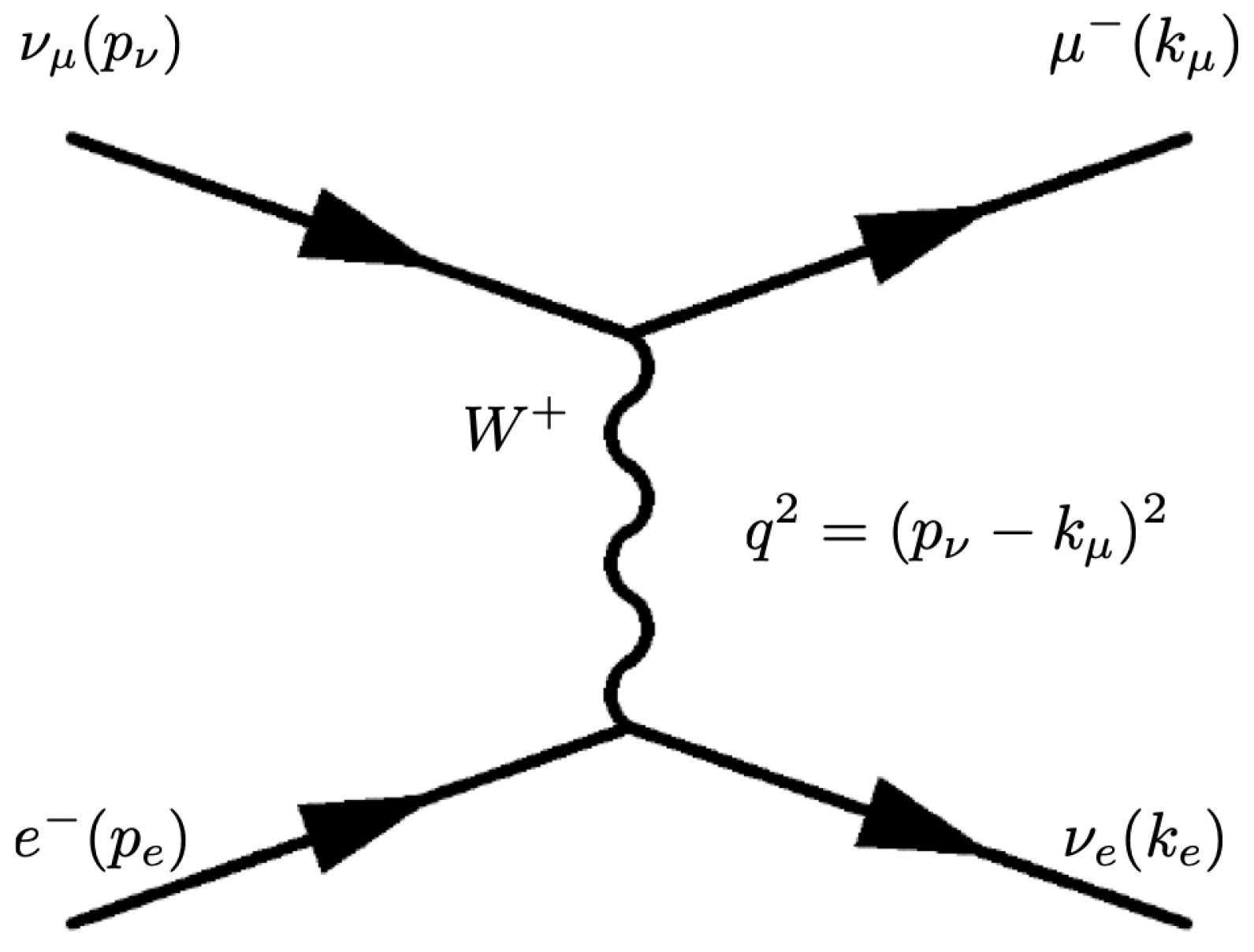
The cross section for the interaction depicted in Figure 1 where a muon neutrino interacts with an electron to form an electron neutrino and muon, as a function of neutrino energy can be written simply as

σ \approx \frac{2 m_{e} G_{F}^{2} E_{ν}}{π} = \frac{G_{F}^{2} s}{π}

(6)

However, to compute cross sections at high, or ultra-high energies such as that of cosmic rays, we have that

\begin{matrix} \frac{d σ (ν_{e})}{d y} = \frac{m_{e} G_{F}^{2} E_{ν}}{2 π} ({(g_{V} - g_{A})}^{2} + \\ (g_{V} - g_{A}^{2}) {(1 - y)}^{2} - (g_{V}^{2} - g_{A}^{2}) (\frac{m_{e} y}{E_{ν}}) \end{matrix}

(7)

where,

G_{F} = \frac{g^{2}}{4 \sqrt{2} M_{W}^{2}} \approx 1.166 \times 10^{- 5} {GeV}^{- 2}

y = 2 m_{e} E_{ν}

which is the outgoing leptonic energy, bounded by

0 \leq y \leq y_{m a x} = 1 - \frac{m_{l}^{2}}{2 m_{e} E_{ν} + m_{e}^{2}}

. The coupling constants are given as

g_{L} = + 1 / 2, g_{R} = 0, g_{V} = + 1 / 2

and

g_{A} = + 1 / 2

in which case

L, R, V, A

are the left, right, vector and axial components, respectively [7].

We can then determine approximate cross-sections for high and ultra high energy cosmic rays. First, by substituting in our components

m_{e} = 9.11 \times 10^{- 31} kg

, with an energy of

300 GeV

we obtain a value for y of

\sim 5.466 \times 10^{- 28}

which gives an approximate cross-section of

5.072 \times 10^{- 34} {cm}^{2}

. Next, we can compare that with an energy level of

500 GeV

0.5 TeV

. This gives us a y value of

\sim 9.11 \times 10^{- 28}

in which we deduce a cross-section of approximately

8.453 \times 10^{- 34} {cm}^{2}

. Lastly we will use an energy of

E_{ν} = 1,000 GeV

1 TeV

, which is the energy level used in determining our cosmic ray probability calculations. The component y we find to be on the order of

\sim 1.822 \times 10^{- 27}

. This yields an approximate neutrino cross section for cosmic rays as approximately

1.691 \times 10^{- 33} {cm}^{2}

3. Oscillation and the Mean Free Path

By using a conversion probability function, we should be able to determine the travel distance for oscillation and predict what state our neutrino should be in at a particular position and time. For this, it is much simpler if we think of oscillating neutrinos as wave packets in some arbitrary state,

ψ

. This arbitrary state is our initial condition in which we have

ψ_{α}

where,

α

is the flavor eigenstate pre-measurement (or detection),

ν_{e}, ν_{μ}, ν_{τ}

. Similarly,

ψ_{α}^{'}

is our final state after detection. We must also consider the probability of measurement of the mass eigenstate. For the sake of simplification, we use the definition for neutrino flavor states as explained by Blasone, et al. (2022) [8], and utilizing the

3 \times 3

Pontecorvo-Maki-Nakagawa-Sakata [PMNS] unitary mixing matrix [9],

U (\tilde{θ}, δ)

, as follows:

{\underset{̲}{ν}}^{(f)} = U (\tilde{θ}, δ) {\underset{̲}{ν}}^{(m)}

(8)

It is imperative to note, that in the above equation, we must explicitly show that there are two possible eigenstates:

{\underset{̲}{ν}}^{(f)}

is our flavor eigenstate representing the transpose of

(ν_{e}, ν_{μ}, ν_{τ})

. Then we have that

{\underset{̲}{ν}}^{(m)}

is our mass eigenstate, which is represented by the transpose of

(ν_{1}, ν_{2}, ν_{3})

. The probability for the flavor transition

ν_{α} \to ν_{β}

[2] can be defined as

P_{ν_{α} \to ν_{β}} (t) = | ν_{β} ν_{α} (t) |^{2} = {| {\tilde{U}}_{α β} (t) |}^{2}

(9)

This indicates the flavor transition at time,

t = 0

with the contribution from [8]. Here we can assume from earlier that our variables,

α

and

β

, can represent any of the flavors

(e, μ, τ)

and we have that

\tilde{U} (t = 0)

is normalized [8].

We know from above that our neutrino flavor mixing matrix can be written as

(\begin{matrix} ν_{e} \\ ν_{μ} \end{matrix}) = (\begin{matrix} cos θ & sin θ \\ - \sin θ & cos θ \end{matrix}) (\begin{matrix} ν_{1} \\ ν_{2} \end{matrix})

(10)

We can now show this as a unitary mixing matrix

U (θ) = (\begin{matrix} cos θ & sin θ \\ - \sin θ & cos θ \end{matrix})

(11)

Assuming that neutrinos can oscillate into three, four or even infinitely many flavors, we can simply demonstrate the phenomenon of mixing by considering a state of two flavors. Note in the above we considered neutrinos to be flavor states as opposed to a combination of mass eigenstates,

ν_{1}, ν_{2}, ν_{3}

. With this in mind, we can consider two weak eigenstates,

ν_{e}

and

ν_{μ}

. Their plane wave forms [2] can be expressed as

ν_{1} (t) = ν_{1} e^{i (p_{1} \cdot x - E_{1} t)} = e^{- i p_{1} \cdot x}

(12)

and also

ν_{2} (t) = ν_{2} e^{i (p_{2} \cdot x - E_{2} t)} = e^{- i p_{2} \cdot x}

(13)

If we let A be the flavor eigenstate consisting of

e, μ, τ

and let B be the neutrino mass eigenstate consisting of

m_{1}, m_{2}, m_{3}

then we must consider that

A \times B \neq B \times A

. Assuming this constraint we can deduce that

A \times B = {(e, m_{1}), (e, m_{2}), (e, m_{3}), (μ, m_{1}), (μ, m_{2}), (μ, m_{3}), (τ, m_{1}), (τ, m_{2}), (τ, m_{3})}

. Similarly,

B \times A

= {(m_{1}, e), (m_{2}, e),

(m_{3}, e), (m_{1}, μ), (m_{2}, μ), (m_{3}, μ), (m_{1}, τ), (m_{2}, τ), (m_{3}, τ)}

. Again we must stress the importance that for this assumption, the probability of A does not depend on the probability of B and the probability of B certainly does not depend on the probability of A. Meaning, if we determine a state in A, that does not mean we know for certain state B but that all other probabilities for state B go to zero.

To consider the probability of an arbitrary neutrino state prediction, we must first consider a known constraint. To make a prediction based on a flavor eigenstate, we must assume that all mass eigenstate probabilities collapse. Conversely, if we are to make a prediction based on a mass eigenstate, all the flavor eigenstate probabilities collapse.

However, we must consider our neutrino eigenstates:

ν_{e}, ν_{μ}, ν_{τ}

and

m_{1}, m_{2}, m_{3}

. Because we are aware of our constraints, the same assumption made previously strictly applies here. That is the outcome observed for A does not depend on the outcome observed for B and the outcome observed for B does not depend on the outcome observed for A.

We can now determine the probability for flavor transition from

ν_{e} \to ν_{μ}

which corresponds to the detection of

ν_{e}

and is dependent on

Δ m

as the mass difference where,

Δ m_{i j}^{2} = m_{i}^{2} - m_{j}^{2}

, E as the neutrino energy and the distance from the source, L.

P (ν_{τ} \to ν_{λ}) = 1 - s i n^{2} (2 θ_{43}) s i n^{2} (\frac{1.27 Δ m_{43}^{2} [e V] L [m]}{E [M e V]})

(14)

Alternatively, we can show the probability of our mass eigenstate and the prediction of the flavor state remaining in

ν_{e}

. We will reserve component,

λ

, as an arbitrary flavor state. The constraint here, however, is certainty in one eigenstate negates certainty in the other [2].

For comparative purposes, on Earth, we can expect a solar neutrino flux on the order of

\sim 5.9 \times 10^{14} m^{- 2}

with approximately

1.7 \times 10^{38}

neutrinos being emitted every second. Considering the type II supernova, SN1987A, located in the Large Magellanic Cloud, was first detected on February 23, 1987. During its luminosity peak, approximately

5.9 \times 10^{19}

neutrinos were detected on Earth per second with an average flux of approximately

1.3 \times 10^{14} m^{- 2}

. The distance d from SN1987A to Earth is

\sim 168,000

light years [10].

4. Sterile Neutrinos

As we consider the neutrino’s ability to oscillate among

ν_{e}, ν_{μ}, ν_{τ}

, it is theoretically possible for the neutrino to oscillate into a heavier fourth flavor with no further oscillations if this fourth flavor can only interact with gravity. Because of this characteristic, this fourth flavor has received the name sterile neutrino. It is important to note that the sterile neutrino was independent of the other three flavors. As a neutrino is created, it is considered to be a superposition of all three flavors and all three masses. This does not include the sterile neutrino. However, similar to a neutrino, a sterile neutrino carries no charge and has a half-integer spin. As mentioned previously, this neutrino would be heavier than the three known masses, and it is theorized to have a mass anywhere between 10 GeV and 1 eV [11].

When we consider the existence of a sterile neutrino, we must also consider the probability of it being categorized as a Majorana particle. A fermion is considered Majorana when it is found to be its own antiparticle. Typical fermions are categorized as Dirac fermions at low energies, with the exception of the neutrino. Dirac fermions do not possess their own antiparticles. At this point, which category the sterile neutrino fits is unknown. If sterile neutrinos are Majorana, when two sterile neutrinos collide, they would annihilate each other with an enormous amount of energy.

We classify these particles as fermions, i. e., with a half-integer spin. In the context of neutrinos, this means their spin may either be

1 / 2

- 1 / 2

depending on the spin quantum number s quantifying direction of intrinsic rotation. Neutrinos are typically considered to be “left-handed" fermions, i.e., with Dirac spinor representations that can be expressed as projections by the left-handed projection operator

P_{L} = \frac{1 - γ^{5}}{2}

. Moreover, the

W^{\pm}

bosons mediating weak interactions involving neutrinos only interact with left-handed particles. When considering sterile neutrinos, they are assumed to be “right-handed" fermions, thus confirming the existence of a positive-spin neutrino.

If we take the mass of one “hand," multiplied by the other “hand" we would deduce a constant mass.

So we can show that:

(R i g h t H a n d M a s s) \times (L e f t H a n d M a s s) = C o n s t a n t

(15)

Therefore, we can now assume that if we were to increase the mass of one hand, that is, left or right, the other hand must become smaller. This results in a process referred to as the “Seesaw Mechanism" [11]

M_{(ν)} = (\begin{matrix} ν_{L} f & ν y \\ ν y & ν_{R} f \end{matrix})

(16)

where, f directly corresponds to neutrinos of heavier mass, however, a mixture of f results in neutrinos of lighter mass [11]. This yields the mass eigenstate of

M_{(ν)} = (\begin{matrix} 0 & M_{D} \\ M_{D} & M_{N H L} \end{matrix})

(17)

in which the mass hierarchy can be shown as

M_{ν} > > M_{D} > > M_{N H L}

, where

M_{ν}

is the neutrino mass,

M_{D}

is the mass of the corresponding deuteron and

M_{N H L}

represents the neutral-heavy lepton [11]. By the Seesaw Mechanism, this yields an approximate neutrino mass of

M_{ν} = \frac{M_{D}^{2}}{M_{N H L}}

(18)

Once again, the Seesaw Mechanism shows that if these right-handed sterile neutrinos exist, they could in fact be categorized as Majorana, which could help explain the difficulty in detecting them. This mechanism gives us a matrix theorizing six neutrino fields, three of which would have masses

< 1 eV

while the other three would have masses

> 1 eV

. Unlike other fermions, these Majorana particles do not exhibit intrinsic electric or magnetic moments. Instead, they would possess toroidal moments in which the field of the solenoid is bent into a torus.

5. Methods

We have previously shown the high probability of detecting our neutrino to be in states,

ν_{e}

ν_{μ}

. To consider a higher flavor transition, we must first consider the transition from

ν_{μ}

ν_{τ}

whose probability can be shown as [2]

P (ν_{μ} \to ν_{τ}) = {sin}^{2} (2 θ_{32}) {sin}^{2} (\frac{1.27 Δ m_{32}^{2} [e V] L [m]}{E [M e V]})

(19)

We now need to expand the PMNS matrix [9] to include a fourth flavor by considering that:

\begin{matrix} | m_{e e} |_{4 ν} = | Σ | U_{e j} |^{2} e^{i ϕ_{j}} m_{j} | = \\ | c_{13}^{2} c_{12}^{2} c_{14}^{2} m_{1} + c_{13}^{2} c_{12}^{2} c_{14}^{2} e^{i α} m_{2} \\ + s_{13}^{2} c_{14}^{2} e^{i β} m_{3} + s_{14}^{2} e^{i γ} m_{4} \end{matrix}

(20)

\begin{matrix} m_{e e} = | Σ | U_{e j} |^{2} e^{i ϕ_{j}} m_{j} | = \\ | c_{13}^{2} c_{12}^{2} c_{14}^{2} m_{1} + c_{13}^{2} c_{12}^{2} c_{14}^{2} e^{i α} \sqrt{m_{1}^{2} + Δ_{21}} \\ + s_{13}^{2} c_{14}^{2} e^{i β} \sqrt{m_{1}^{2} + Δ_{31}} + s_{14}^{2} e^{i γ} \sqrt{m_{1}^{2} + Δ_{41}} \end{matrix}

(21)

(\begin{matrix} ν_{e} \\ ν_{μ} \\ ν_{τ} \\ ν_{λ} \end{matrix}) = (\begin{matrix} U_{e 1} & U_{e 2} & U_{e 3} & U_{e 4} \\ U_{μ 1} & U_{μ 2} & U_{μ 3} & U_{μ 4} \\ U_{τ 1} & U_{τ 2} & U_{τ 3} & U_{τ 4} \\ U_{λ 1} & U_{λ 2} & U_{λ 3} & U_{λ 4} \end{matrix}) (\begin{matrix} ν_{1} \\ ν_{2} \\ ν_{3} \\ ν_{4} \end{matrix})

(22)

where

U = R_{34} R_{24} R_{14} R_{23} R_{13} R_{12} P

and so that [9] ,

\begin{matrix} R_{14} = (\begin{matrix} c_{14} & 0 & 0 & - s_{14} e^{i δ_{14}} \\ 0 & 1 & 0 & 0 \\ 0 & 0 & 1 & 0 \\ - s_{14} e^{i δ_{14}} & 0 & 0 & c_{14} \end{matrix}) a n d \\ R_{34} = (\begin{matrix} 1 & 0 & 0 & 0 \\ 0 & 1 & 0 & 0 \\ 0 & 0 & c_{34} & s_{34} \\ 0 & 0 & - s_{34} & c_{34} \end{matrix}) \end{matrix}

(23)

We can now define the probability for a higher-order transition as

P (ν_{τ} \to ν_{λ}) = {sin}^{2} (2 θ_{43}) {sin}^{2} (\frac{1.27 Δ m_{43}^{2} [e V] L [m]}{E [M e V]})

(24)

where,

L [m]

is the distance from the source,

E [M e V]

is the energy and

Δ m

is the mass difference between the flavors during the oscillation. This indicates that the probability of finding a neutrino in the fourth flavor state should be equal to the probability of finding it in the third flavor state.

Taking what we know from our probability functions, Equations

(12)

and

(19)

, we can now use this to determine the probability for an

n^{t h}

flavor. If we assume an oscillation into a fourth flavor, the sterile neutrino, is probable, then we can assume an equal probability of continuous oscillation into n flavors. We can now determine the theoretical travel distance for oscillation from

ν_{e} \to ν_{μ}

by assuming our mixing angle

θ

to be

\sim 0.846

, our

| Δ m_{21} |^{2}

to be approximately

7.4 \times 10^{- 5} {(eV / c^{2})}^{2}

and we can assume an approximate energy E of

10^{8} eV

assuming a supernova neutrino creation. We can show a travel distance of approximately

10^{21} m

or around

105,700

light years, with a probability of

\sim 1

\sim 100 %

of the transition from electron neutrino,

ν_{e}

, to muon neutrino,

ν_{μ}

. Given this amount of travel distance, the neutrino would have definitively transitioned from its electron state, to its muon state.

To ascertain the pattern of transitional probabilities, a Python program was developed to compare transitions between three widely detected neutrino types: solar, supernova and cosmic rays. For our first simulation, the following parameters were used for solar neutrinos:

For the first flavor change we will use for our mixing angle,

{sin}^{2} θ \approx 0.846

and a mass difference of

Δ m_{21}^{2} \approx 7.40 \times 10^{- 5} {eV}^{2}

. For our second flavor change,

{sin}^{2} θ \approx 0.92

and

Δ m_{32}^{2} \approx 2.40 \times 10^{- 3} {eV}^{2}

. For our third flavor change,

{sin}^{2} θ \approx 0.994

and

Δ m_{43}^{2} \approx 0.05 {eV}^{2}

. With an adopted solar neutrino energy of

E [M e V] \approx 1 MeV

6. Results

We are now in a position to use our expression for neutrino transitional probabilities to estimate the neutrino transition fractions (among 3 species) at various distances. First we turn to our most important neutrino source, the Sun. The transitional probabilities from

ν_{e} \to ν_{μ}

and

ν_{μ} \to ν_{τ}

are shown in Table 1 for solar neutrinos.

For Table 2, we maintain the parameters used above and apply them to neutrinos detected from supernova events. We assume a median supernova neutrino energy level of

\sim 10 MeV

Finally, in Table 3, we consider a significant increase in energy. This is partly due to the first- and second- order Fermi processes within the magnetized clouds accelerating the cosmic rays. With this in mind, and again utilizing our base parameters, we now have an increased cosmic ray energy of

\sim 1 \times 10^{6} MeV

From the above tables, we have shown the distance needed to oscillate from the first flavor to the second flavor, with a consistently high probability of transition. Once we move into the second, third, and

n^{th}

flavors, we become less certain about our flavor transition probabilities. From the above two tables, we can infer why this is the case. We can clearly see that our probabilities for the higher flavors

(μ \to τ, τ \to λ)

are the lowest when the probability for the transition from the first to the second flavor

(e \to μ)

is at its highest. For example, for a cosmic ray neutrino, using our transition from

ν_{τ} \to ν_{λ}

at distances

10^{5} m

and

10^{10} m

we obtained probabilities of

\sim 0.00 %

and

\sim 12.6 %

, respectively.

When comparing this with our probability from

ν_{e} \to ν_{μ}

at the same distances, we find a probability of

99.9 %

but a significant decease to

\sim 35.8 %

when

ν_{μ} \to ν_{τ}

\sim 60.2 %

. However, in Tables 1 and 3 there are distances from which our first flavor transition is approximately equal to our third flavor transition. In the case of Solar neutrinos, at

L [m] \sim 10^{20} m

the probabilities for first and third transitions are

\sim 44.9 %

and

\sim 45.7 %

, respectively. For the case with cosmic rays, we have that at

L [m] \sim 10^{27} m

our first transition is

\sim 60.5 %

while our third transition is

\sim 66.7 %

If we consider our distance of travel to be on the order of 1 AU Unit (AU), we find that our probability would be

\sim 0.261

for flavor oscillation into the second state and

\sim 0.111

for higher-order flavor transitions. When we compare this to known detection rates, we find approximately

\frac{2}{3}

of detected neutrinos from the Sun to found in either

ν_{e}

ν_{μ}

flavor state, which is consistent with our findings in the range of

\sim 26.1 %

found in the

ν_{e}

flavor state [12].

A similar assumption can be made for atmospheric neutrinos. As cosmic rays bombard the atmosphere of Earth, protons strike the nuclei of atoms within our atmosphere forming pions. These short-lived particles decay into muons which then leave behind an electron, anti-electron and a neutrino, the

ν_{μ}

. This flavor, according to Fermilab, make up approximately

\frac{2}{3}

of the detected neutrinos on Earth leaving behind

\frac{1}{3}

to be detected as

ν_{e}

[1]. When comparing this with our calculations, we find that with cosmic rays we expect at a distance of

1.5 \times 10^{11} m

\sim 0.399

to be in flavor state

ν_{e}

, while we have

\sim 0.813

to be in state,

ν_{μ}

Taking these transition probabilities into account, we can quickly see that from varying distances and probabilities, the neutrino oscillation of flavors is simply a cycle of probabilities. In other words, the flavor transition can start again depending on the distance travelled prior to detection. What makes this concept more intriguing is that it helps explain a possible reasoning behind only having certainty in one eigenstate and not in both. When we measure a neutrino in a flavor eigenstate, we can assume that, and as the tables above show, as it oscillates between flavors it becomes a combination of all possible masses

m_{1}, m_{2}, m_{3}, \dots, m_{n}

. When we consider the combination of mass matrices, this also helps to understand the cycle of flavor oscillations prior to detection.

If we are to assume that when we observe a neutrino in state A or

ν^{f}

we have the probability for

ν_{e}, ν_{μ}, ν_{τ}, ν_{λ}

with state B or

ν^{m}

for

m_{1}, m_{2}, m_{3}, m_{λ}

. We can predict our condition to be approximately as observed

ν_{e}

to have state B of

m_{1}, 0, 0, 0

, for

ν_{μ}

we find

m_{1}, m_{2}, 0, 0

, for

ν_{τ}

we would show

m_{1}, m_{2}, m_{3}, 0

and for

ν_{λ}

m_{1}, m_{2}, m_{3}, m_{λ}

. This shows that each potential flavor state can be thought of simply as a combination of all possible masses.

7. Analysis of Results

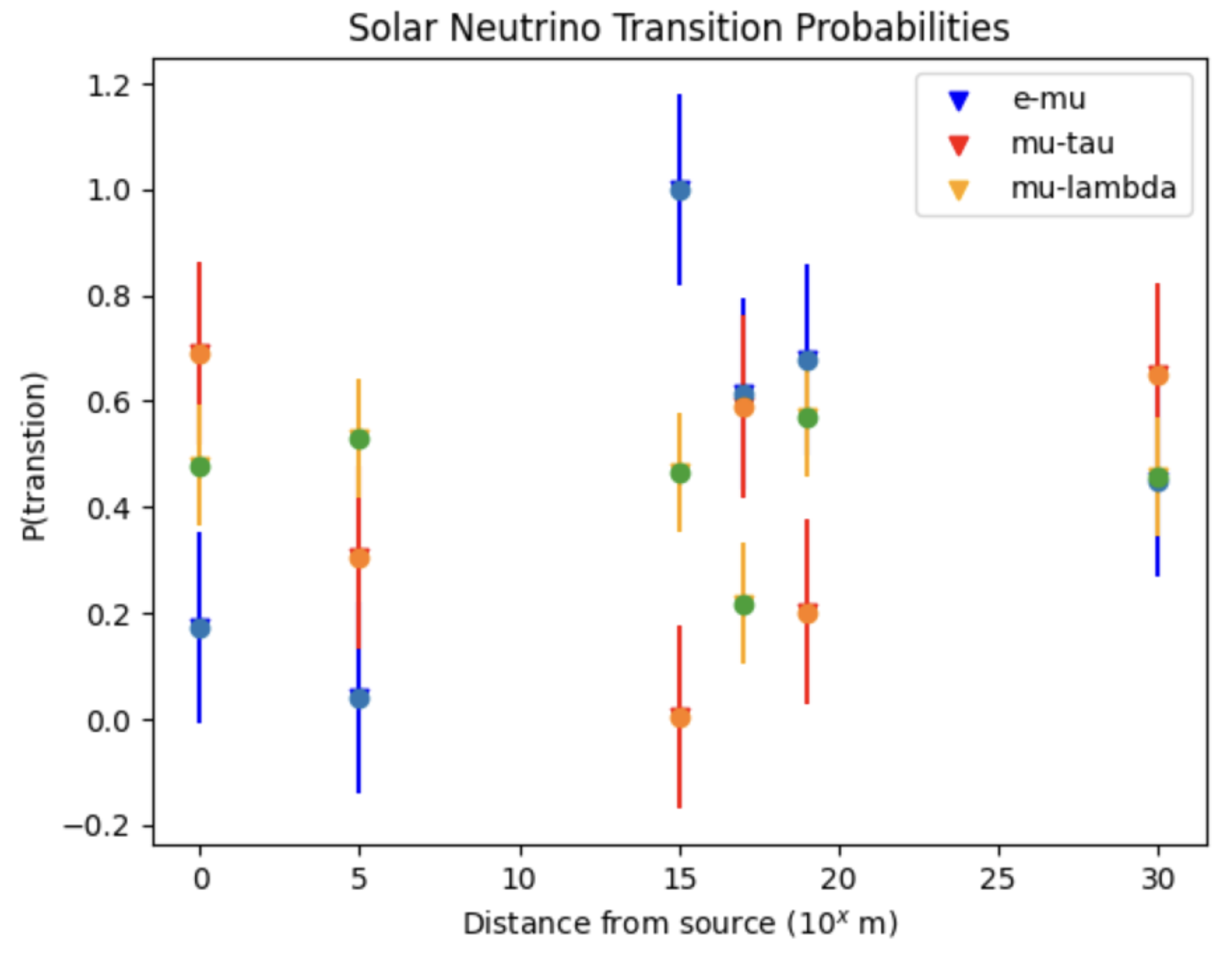
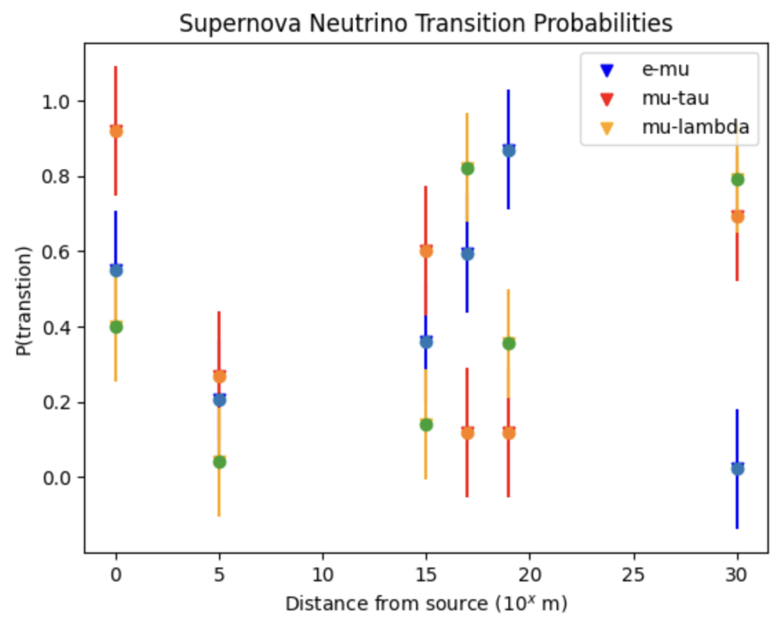
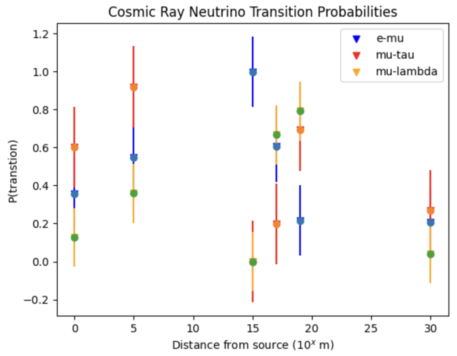
In Figure 2, Figure 3 and Figure 4, we show a comparison between the probabilities of the flavor transitions:

ν_{e} \to ν_{μ}

ν_{μ} \to ν_{τ}

and

ν_{τ} \to ν_{λ}

for solar, supernova and cosmic ray neutrinos, where

λ

is any higher order flavor transition from the

4^{t h} \dots n^{t h}

flavor states. We can see from the probability distribution, that the closer we are to the source, the lower the probability of a higher-order flavor transition, as expected. However, as the neutrino oscillates at greater distances, a pattern of fluctuating probabilities can be observed. We can infer from this that as the neutrino approaches

\sim 10^{25}

m from its source, the probabilities for all three flavors are all three approximations of each other,

\pm 0.10

. With this understanding we can then follow the flavor transition by reverting backward through each flavor culminating at an equivalent point for both

ν_{e}

and

ν_{μ}

. From there, and as the neutrino oscillates further, we can then assume a probability for the first flavor as it approaches the probability for the

n^{t h}

flavor transition; in this case, the sterile neutrino.

From the data in the figures above, we can ascertain that at a certain point, the probability of a neutrino oscillating into a fourth flavor state after a certain distance approaches the probability that the neutrino is being found in its first flavor state. This further shows that each flavor can be thought of as a proper combination of all mass and flavor eigenstates oscillating back and forth between states. The probability of oscillating into a higher

n^{t h}

flavor is approximately the same as that of the neutrino oscillating backward through the previous states and beginning the cycle.

We can see in Figure 2, as the solar neutrino has travelled

\sim 10^{27}

m from its source, the probability of it being found in the electron state is approximately the probability of it being found in its lambda state. From Figure 3, we can see the same equivalency; however with a supernova neutrino the distance is now

\sim 10^{20}

m. With higher-energy neutrinos, such as those in Figure 4, we can see a unique symmetry between all three flavor of neutrino states. Here we can see where one flavor has a high probability, and the other two are at their lowest, and vice versa.

When we consider the neutrino’s mean free path of

\sim 105,700

light years, or

10^{21}

m from its source, we can see that this fits perfectly with the neutrino energy stemming from supernova neutrinos. However, when we focus on the lower-energy solar neutrinos, we find that given a slightly further distance of travel (

10^{27}

m), we arrive at a near

0.5

probability of detecting our neutrino in the first and fourth flavor states. An inference here tells us that the lower-energy neutrinos, given a longer distance of oscillation, have a higher probability of oscillating back through and begins the cycle over again. higher-energy levels tend to oscillate much faster, creating a uniquely consistent probability distribution for flavor transformations.

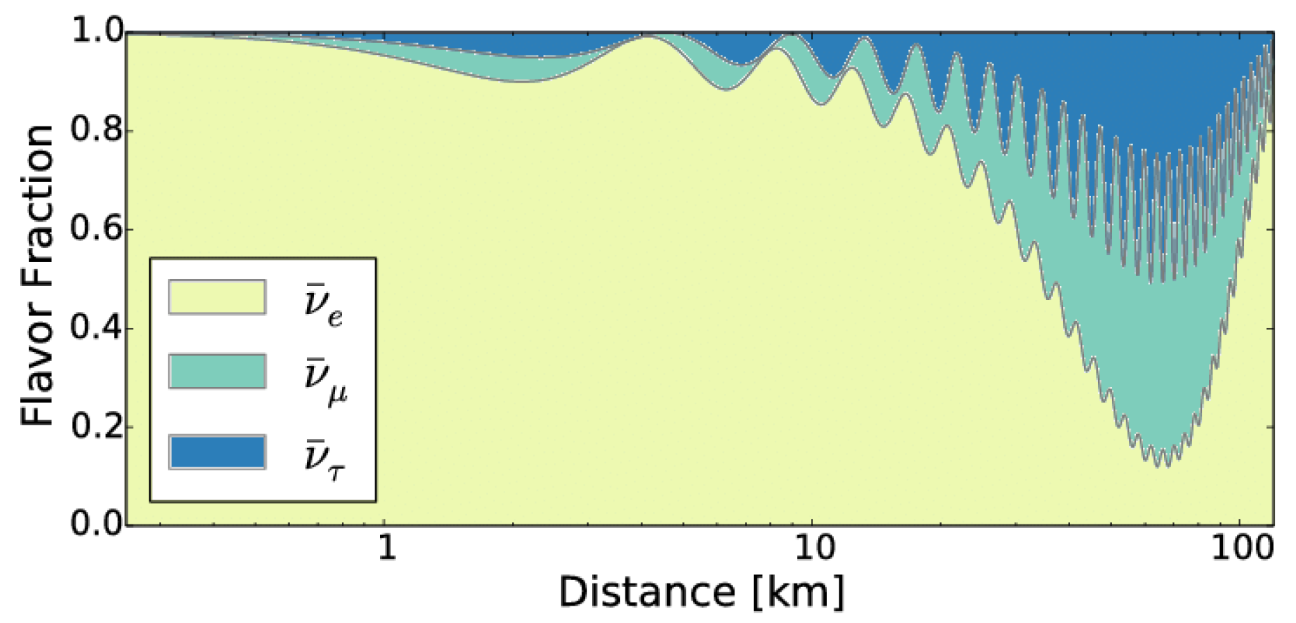
From Figure 5, we can see the flavor fraction of detected neutrinos at the Reactor Experiment for Neutrino Oscillations (RENO) in South Korea[13]. When comparing this data to our above probabilities, and adjusting for unit of distance conversions, we find that for solar neutrinos at approximately 50 km we deduce a probability of

ν_{e} \sim 0.985

ν_{μ} \sim 0.928

and

ν_{τ} \sim 0.696

and at 75 km

ν_{e} \sim 0.473

ν_{μ} \sim 0.419

and

ν_{τ} \sim 0.020

. In comparison with supernova neutrinos we find that at the same distances we have probabilities of

ν_{e} \sim 0.202

ν_{μ} \sim 0.189

and

ν_{τ} \sim 0.0.33

and at 75 km

ν_{e} \sim 0.473

ν_{μ} \sim 0.542

and

ν_{τ} \sim 0.763

. Based on the above data, and our previous calculations the probability for cosmic ray neutrinos remain on the order of

10^{- 5}

until it reaches an approximate distance of

\sim 1 \times 10^{5}

m or 100 km which is also shown in the above fraction distribution. These observations were conducted at RENO in South Korea. 2023 began new observations at JUNO in Guangdong, Southern China. Observations should be concluded late 2024-early 2025. It will be of great interest to note any similarities and/or differences in the observations.

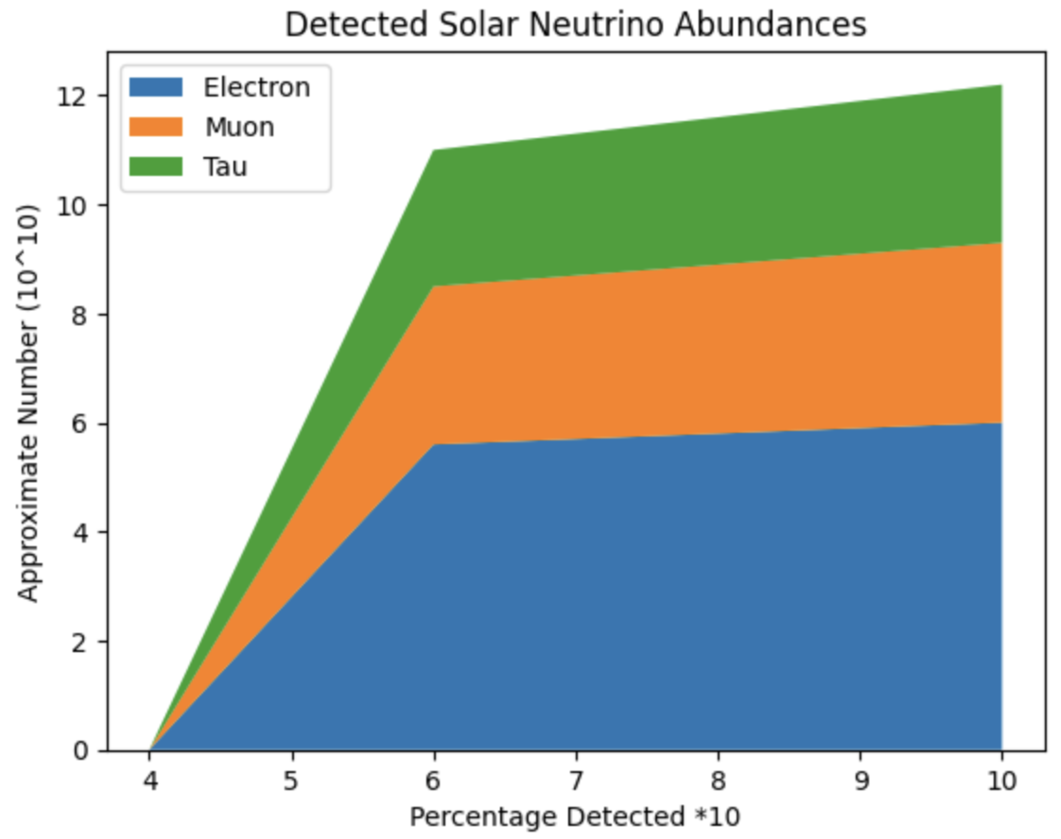
The density chart described in Figure 6 was calculated using a predicted flavor contribution to the solar neutrino flux detected on Earth. With an oscillation distance of

L_{E} = 1.5 \times 10^{11}

meters, we find our changes to neutrino flavor abundance (number density) with distance for each observed flavor to be

\frac{Δ}{Δ L} < n_{ν_{e}}, n_{ν_{μ}}, n_{ν_{τ}} > \approx < n_{0} (1 - P_{12}), n_{0} P_{12} (1 - P_{23}), n_{0} P_{12} P_{23} (1 - P_{3 λ}) >

where,

n_{0}

is the original number density of electron neutrinos emitted from proton-proton chains within the Sun which is approximately

6.0 \times 10^{10} {cm}^{2}

and

P_{m n}

are the corresponding flavor transition probabilities.

The neutrino flux can be found by

\frac{2 L_{S u n}}{28 M e V} \frac{1}{4 π d^{2}} / {cm}^{2} \approx 6.0 \times 10^{10} {cm}^{2} s^{- 1}

. With an oscillation distance on the order of one AU,

10^{11}

meters, we find the number of detected flavors we can expect on Earth from the Sun to be approximately

1.158 \times 10^{11}

neutrinos per square meter per second.

When comparing our probability density with the observed fraction density taken by RENO in South Korea [13], we can see that our predicted flavor detection at much greater distances, closely resembles those observed by RENO at a tenth of the distance from the Sun. This tells us that within distances of approximately

100,000 - 1,500,000

meters, our probabilities give us great confidence in our ability to predict flavor transitions over great distances.

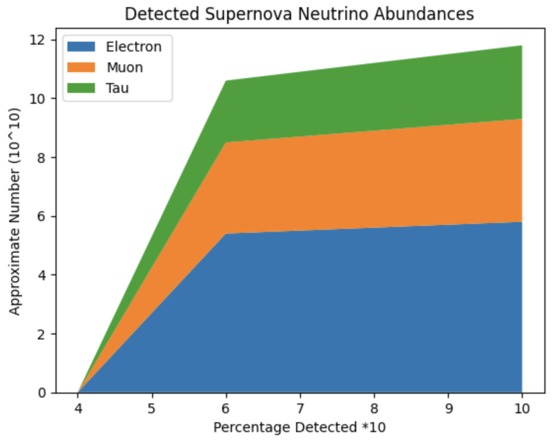
For comparative purposes, tables for both supernova neutrinos as well as those from cosmic rays were constructed using similar methods. However for the tables below, a supernova distance of

1.6 \times 10^{21} m

was used and for the cosmic rays a shorter distance of

\sim 10^{11} m

was used for these particular densities.

Figure 7. The above image shows the fraction of predicted supernova neutrino flavor detection given an oscillation distance of

1.6 \times 10^{21}

Figure 7. The above image shows the fraction of predicted supernova neutrino flavor detection given an oscillation distance of

1.6 \times 10^{21}

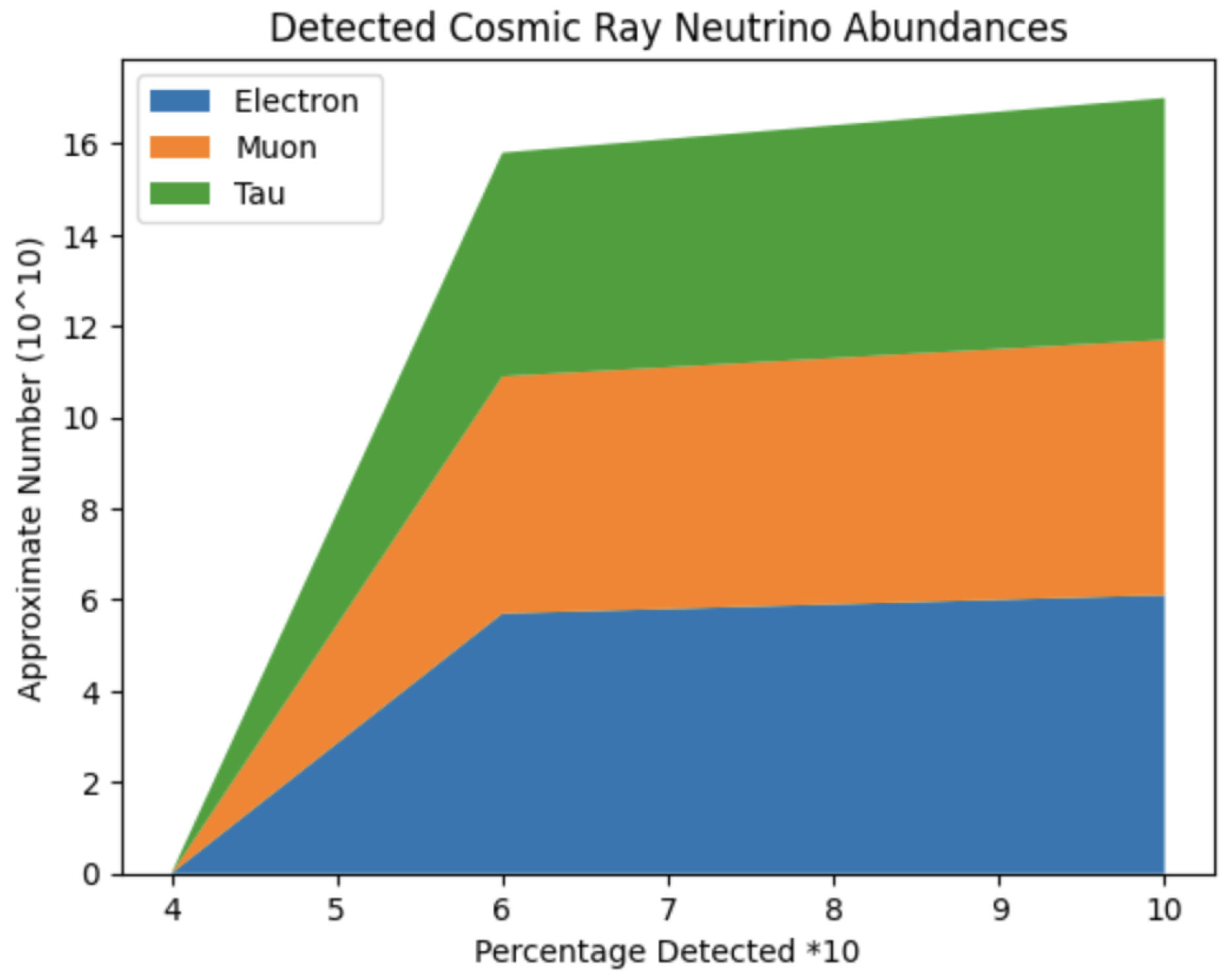
Figure 8. The above image shows the fraction of predicted cosmic ray neutrino flavor detection given an oscillation distance of

\sim 10^{11}

Figure 8. The above image shows the fraction of predicted cosmic ray neutrino flavor detection given an oscillation distance of

\sim 10^{11}

We found that for the supernova neutrinos, around

50 %

should be detected as electron neutrinos while

\sim 30 %

to be detected as muon neutrinos and the final

20 %

should be detected as tau neutrinos. Interestingly for the cosmic ray neutrinos, we found that approximately

36 %

should be detected as electron neutrinos,

33 %

as muon neutrinos and

31 %

as tau neutrinos.

8. Discussion

In this paper we have shown that we can determine the probabilities of neutrino flavor states by first calculating the product of flavor eigenstate and then mass eigenstate probabilities. We found that the greater the distance from the source, the higher the probability of finding the neutrino in a different state than that in which it was produced. We found that for solar neutrinos,

10^{5} m

from the source, the neutrino has a

99.9 %

chance of being detected in the state,

ν_{μ}

, and a

46.4 %

chance of oscillating into a fourth flavor or simply reverting backwards. We find that at around

10^{27} m

this process starts over again. For supernova neutrinos, we find that at the same distances, we expect to find

ν_{τ}

with a

60.2 %

chance and

ν_{e}

with a

35.8 %

chance. This time at around

10^{25} m

we find the process starting again. For the higher-energy cosmic rays, we find a similarity between the probabilities of that and the solar neutrinos. When comparing at the same distances, we have

99.9 %

chance of detection in the state,

ν_{e}

and a

0.00 %

chance of higher flavor transitions. Again, back to our distance of

10^{27} m

, we find the process starts again.

In repeating the same process, but for a distance of one AU unit, or

1.5 \times 10^{11} m

we found that our neutrino flux should be comprised of approximately

50 %

electron-neutrinos,

26.7 %

muon-neutrinos and

23 %

tau neutrinos. When we extend this distance a bit further for supernova we found approximately,

48 %

32 %

and

20 %

electron-, muon- and tau-neutrinos, respectively. When considering higher-energy cosmic rays at a distance of approximately

10^{11} m

we found a surprising split between

36 %

33 %

and

31 %

for the electron-, muon- and tau-neutrinos. We have shown with minimal assumptions on well-established neutrino transition probability function that neutrino population statistics differ significantly among astrophysical sources. Both Solar and supernova neutrino populations detected on Earth are relatively

ν_{e}

-dominant, whereas higher-energy cosmic ray neutrinos that are candidates for Ice Cube, Super Kamiokande and future planned detectors have a relatively uniform flavor distribution.

So far, only three flavor states have been detected, however we have shown that the likelihood of oscillating into a fourth flavor is equal to the oscillation back through the previous flavors,

ν_{τ} \to ν_{μ} \to ν_{e}

. This raises an important question: since we know the flavors are linear combinations of the mass eigenstates, is it possible for a fourth flavor transition or would the neutrino’s transformation cease at the

ν_{τ}

and simply revert back to the first flavor state?

More succinctly put, if we measure in the flavor state we cannot determine the mass state except for a linear combination of all possible masses. In future work, we may test if the assumption of non locality implies that the reverse case of mass eigenstates being expressible as flavor eigenstates could be true as well. We determined that when considering the probabilities of detecting states, we can make predictions based off of a distance travelled since creation. In doing so, we found that a neutrino not only has a probability near unity of oscillating further but also oscillating backward into prior states. This leaves room for more research to primarily focus attention on the mass eigenstates and determine whether the combination of masses can mimic other flavors and vice versa.

Author Contributions

Conceptualization, John Harrison; Data curation, John Harrison; Formal analysis, John Harrison; Funding acquisition, Richard Anantua; Investigation, John Harrison; Methodology, John Harrison; Resources, John Harrison and Richard Anantua; Software, John Harrison; Supervision, Richard Anantua; Validation, Richard Anantua; Visualization, John Harrison; Writing – original draft, John Harrison; Writing – review & editing, Richard Anantua.

Funding

This work was supported by a grant from the Simons Foundation (00001470, BC, RA).

Acknowledgments

The authors wish to thank Dr. Joseph A. Formaggio at MIT and Dr. Petr Vogel at Caltech for their permission to use Figure 1 and Figure 6, respectively.

Conflicts of Interest

The authors declare no conflicts of interest.

References

Fermilab. Big Bang Neutrinos. Available online: https://neutrinos.fnal.gov/sources/big-bang-neutrinos/ (Accessed on 9/9/2023) 2023.
Giunti, C.; Kim, C. Neutrino Physics and Astrophysics, 1st ed., Publisher: Oxford University Press, United Kingdom, 2007.
Bustamente, M., et. al. High-energy cosmic-ray acceleration, CERN, Available online: https://cds.cern.ch/record/1249755/files/p533.pdf (Accessed on 9/10/2023)2009.
CERN. The Standard Model. Available online: https://home.cern/science/physics/standard-model (Accessed 9/2/2023) 2023.
Diwan, M. Neutrino Sources. Available online: https://www.phy.bnl.gov/diwan/talks/pedagogy/diwan-nu-sources.pdf (Accessed on: 1/11/2023) 2018.
Fermilab andRocco,N.NeutrinoCrosssections.Availableonline:https://indico.fnal.gov/event/19346/contributions/51548/attachments/32048/39314/Noemi_Rocco_Lepton_nucleus_cross_section_theory.pdf (Accessedon2/19/2024) 2019.
Formaggio, J. A., Zeller, G.P. From eV to EeV: Neutrino Cross-Sections Across Energy Scales, 2013, arXiv:1305.7513v1 [hep-ph].
Blasone, M.; De Siena, S.; Matrella, C. Non-locality and entropic uncertainty relations in neutrino oscillations. Eur. Phys. J. Plus, 2022, 137, 1272.
Korana, B.S., Nautiyal, V.K. Effective Neutrino Masses From Four Flavor Neutrino Mixing Matrix, 2020, International Journal of Theoretical Physics, 60: 781-792.
Fermilab. Supernova Neutrinos-Fermilab. Available online: https://neutrinos.fnal.gov/sources/supernova-neutrinos/ (accessed on 9/9/2023)2023.
Akhmedov E.; Frigerio M. Duality in left-right symmetric seesaw mechanism. Phys Rev Lett. 2006, 96(6):061802.
Fermilab. Supernova Neutrinos. Available online: https://neutrinos.fnal.gov/sources/supernova-neutrinos/ (Accessed on 9/9/2023)2023.
Vogel, Petr; Wen, Liangjian; Zhang, Chao Neutrino Oscillation Studies with Reactors 2015 Nature Communications 6. 10.1038/ncomms7935.

Figure 1. Feynman diagram depicting the scattering of an incoming muon-neutrino and an at rest electron. Figure used with permission of author [7].

Figure 2. Scatter plot depicting the comparison of probabilities between solar neutrino flavor transitions

ν_{e} \to ν_{μ}

ν_{μ} \to ν_{τ}

and

ν_{τ} \to ν_{λ}

Figure 2. Scatter plot depicting the comparison of probabilities between solar neutrino flavor transitions

ν_{e} \to ν_{μ}

ν_{μ} \to ν_{τ}

and

ν_{τ} \to ν_{λ}

Figure 3. Scatter plot depicting the comparison of probabilities between supernova neutrino flavor transitions

ν_{e} \to ν_{μ}

ν_{μ} \to ν_{τ}

and

ν_{τ} \to ν_{λ}

Figure 3. Scatter plot depicting the comparison of probabilities between supernova neutrino flavor transitions

ν_{e} \to ν_{μ}

ν_{μ} \to ν_{τ}

and

ν_{τ} \to ν_{λ}

Figure 4. Scatter plot depicting the comparison of probabilities between cosmic ray flavor transitions

ν_{e} \to ν_{μ}

ν_{μ} \to ν_{τ}

and

ν_{τ} \to ν_{λ}

Figure 4. Scatter plot depicting the comparison of probabilities between cosmic ray flavor transitions

ν_{e} \to ν_{μ}

ν_{μ} \to ν_{τ}

and

ν_{τ} \to ν_{λ}

Figure 5. The above image shows the fraction of detected neutrino flavors with their corresponding oscillation distance. Figure used with permission of author [13].

Figure 6. The above image shows the fraction of predicted solar neutrino flavor detection given an oscillation distance of

1.5 \times 10^{11}

Figure 6. The above image shows the fraction of predicted solar neutrino flavor detection given an oscillation distance of

1.5 \times 10^{11}

Table 1. Oscillation probabilities from Solar neutrinos at various distances from the source of neutrino production.

Distance $L [m]$	P $(ν_{e} \to ν_{μ})$	P $(ν_{μ} \to ν_{τ})$	P( $ν_{τ} \to ν_{λ})$
$10^{5}$	$0.999$	$0.004$	$0.464$
$10^{10}$	$0.172$	$0.691$	$0.479$
$10^{15}$	$0.041$	$0.304$	$0.528$
$10^{20}$	$0.449$	$0.650$	$0.457$
$10^{25}$	$0.677$	$0.202$	$0.570$
$10^{27}$	$0.612$	$0.591$	$0.218$

Table 2. Oscillation probabilities from supernova neutrinos at various distances from the source of neutrino production.

Distance $L [m]$	P $(ν_{e} \to ν_{μ})$	P $(ν_{μ} \to ν_{τ})$	P( $ν_{τ} \to ν_{λ})$
$10^{5}$	$0.358$	$0.602$	$0.140$
$10^{10}$	$0.548$	$0.919$	$0.399$
$10^{15}$	$0.205$	$0.268$	$0.041$
$10^{20}$	$0.220$	$0.692$	$0.792$
$10^{25}$	$0.868$	$0.117$	$0.355$
$10^{27}$	$0.595$	$0.117$	$0.822$

Table 3. Oscillation probabilities from cosmic ray neutrinos at various distances from the source of neutrino production.

Distance $L [m]$	P $(ν_{e} \to ν_{μ})$	P $(ν_{μ} \to ν_{τ})$	P( $ν_{τ} \to ν_{λ})$
$10^{5}$	$0.999$	$0.000$	$0.000$
$10^{10}$	$0.358$	$0.602$	$0.126$
$10^{15}$	$0.548$	$0.919$	$0.359$
$10^{20}$	$0.205$	$0.268$	$0.041$
$10^{25}$	$0.216$	$0.692$	$0.792$
$10^{27}$	$0.605$	$0.198$	$0.667$

Disclaimer/Publisher’s Note: The statements, opinions and data contained in all publications are solely those of the individual author(s) and contributor(s) and not of MDPI and/or the editor(s). MDPI and/or the editor(s) disclaim responsibility for any injury to people or property resulting from any ideas, methods, instructions or products referred to in the content.

© 2024 by the authors. Licensee MDPI, Basel, Switzerland. This article is an open access article distributed under the terms and conditions of the Creative Commons Attribution (CC BY) license (http://creativecommons.org/licenses/by/4.0/).

Copyright: This open access article is published under a Creative Commons CC BY 4.0 license, which permit the free download, distribution, and reuse, provided that the author and preprint are cited in any reuse.

MDPI Initiatives

Important Links

Choose an area of interest and we will send you notifications of new preprints at your preferred frequency.

Disclaimer

High-Energy Neutrino Flavor State Transition Probabilities

Abstract

1. Introduction

2. Neutrino Cross-Sections

3. Oscillation and the Mean Free Path

4. Sterile Neutrinos

5. Methods

6. Results

7. Analysis of Results

8. Discussion

Author Contributions

Funding

Acknowledgments

Conflicts of Interest

References

MDPI Initiatives

Important Links

Subscribe