On the Numerical Investigation of Natural Convection Heat Sinks Across a Wide Range of Flow and Operating Conditions

Many designs for natural convection heat sinks, and semi-empirical correlations have been proposed in the recent years, but they are only valid in a limited range of Elenbaas number $El$ and were mostly tested for laminar flows. To alleviate those limits, parametric studies with 2D and quasi-3D models were carried out with ranges of Grashof numbers up to $1.55 \cdot 10^{11}$ and Elenbaas numbers up to $3.42 \cdot 10^7$. Ansys Fluent’s laminar, transition-SST, SST k-$\omega$, and k-$\epsilon$ models were applied. In addition, when used in this valid range, \textit{i.e.} mean Elenbaas numbers, with the simplified quasi-3D model, the transition-SST model can predict better results, over-estimating the heat flux by $10$ to $15\%$ compared to semi-empirical correlations. The 2D model was not deemed satisfying regarding turbulence models. Consequently, a quasi-3D model was developed: it appeared to be an efficient trade-off between computational time and prediction accuracy, in particular for turbulence models. New grouping factors were also found, to ensure proper dimensioning of natural convection heat sinks. They correspond to non-dimensional parameters that dictate the physical behaviour of the heat sink with respect to the semi-empirical correlations. Typically, the ratio of the spacing to the optimal spacing predicted by Bar-Cohen's correlation turned out to be an appropriate grouping factor with a threshold of $1$, above which the fins could safely be considered as isolated, thus greatly simplifying all further calculations.

Keywords:

Subject: Engineering - Mechanical Engineering

1. Introduction

As our modern societies rely always more on electronic devices, efficient solutions for cooling must be found. This is very challenging, as those solutions must fulfill many requirements and trade-offs, such as being cheap to manufacture, efficient from a technical point of view, and overall safe. Passive cooling solutions often come forward for those applications, as they do not have any mechanical parts, thus requiring minimal maintenance. In general, they can dissipate between

0.1

and

10 W / {cm}^{2}

, but this value obviously depends on many factors, such as shape, density, materials, etc. [1]. They use natural convection, as opposed to forced convection for active cooling. This value is obviously less than for the active solutions, however they are more energetically efficient since they do not require any source of energy to work. Consequently, they have an extended lifespan, which is why they are often used for devices which will not be monitored physically very frequently, such as remote radio heads. They are silent, which is a clear benefit compared to active cooling appliances, such as pumps or fans, which can be very loud. In addition, they do not require any electrical power to work, which is very beneficial for small devices which have to work remotely for long periods of time with limited power [1].

In addition, safety is of the major concern when dealing with heat dissipation devices, and temperature is by far the major source of failure [2]. It is obviously very detrimental for the heat sink itself, for the device it aims at cooling and for the people around, which is why sufficient heat dissipation capacity should be ensured.

The development of efficient, reliable and low-cost passive cooling solutions is a major stake from the social, economical and environmental point of view. However, as will be discussed later, no results are known for heat sinks for a large variety of conditions, typically for

E l ≳ 10^{5}

G r_{L} ≳ 10^{8}

. Further physical interpretation on those parameters will be provided after.

1.1. Semi-Empirical Correlations for $\bar{N u_{S}}$

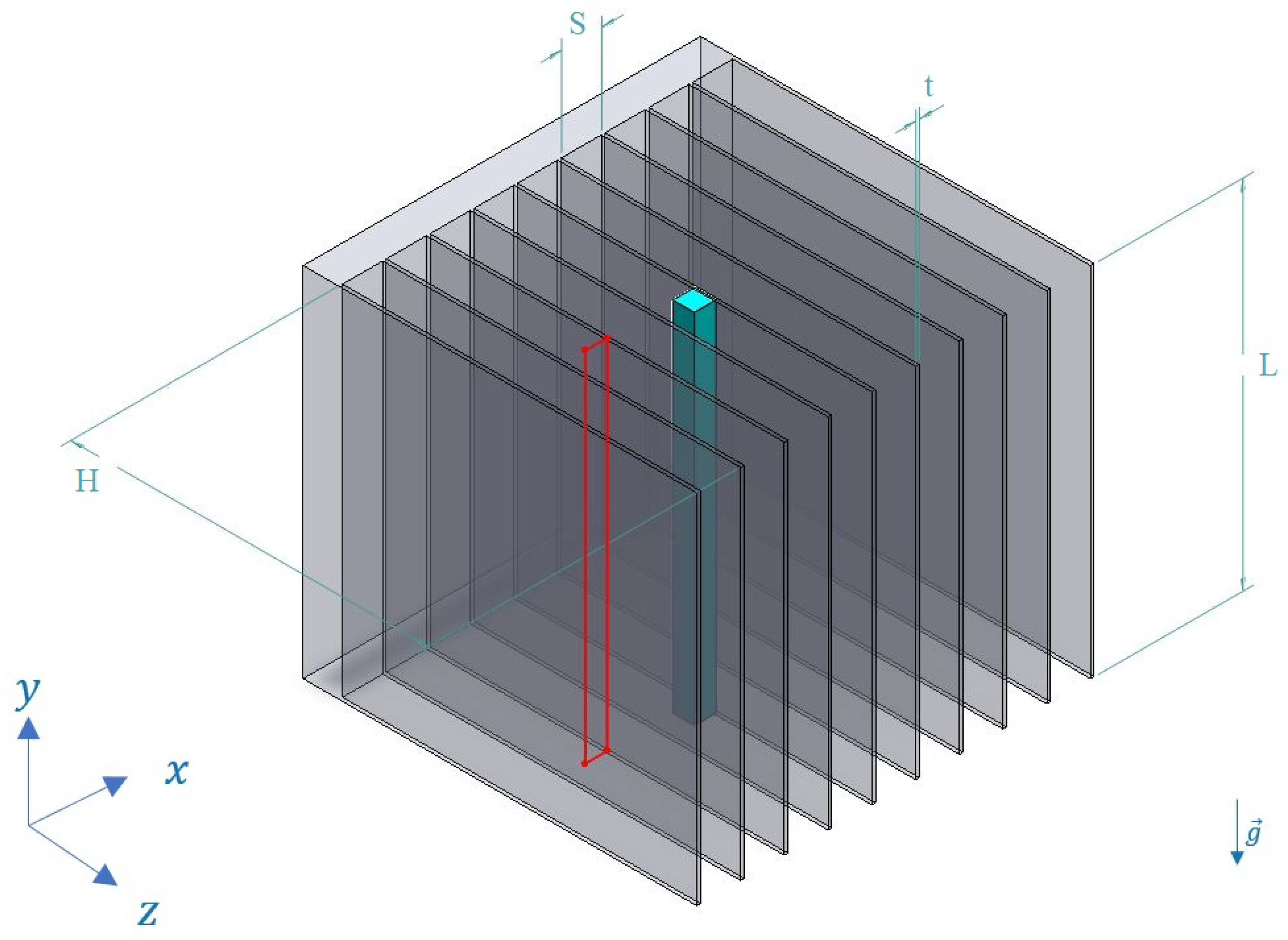
This article focuses on vertical plate-fin heat sinks, i.e., an array of rectangular fins periodically placed on a baseline that is also rectangular. The definitions of the dimensions are shown in Figure 1. S is the spacing between two adjacent fins, L is the vertical length and t is the thickness of a fin, which will be fixed here.

The heat transfer through these natural convection heat sinks is calculated using the average Nusselt number defined as:

\bar{N u_{S}} = \frac{h S}{k},

(1)

where h is the heat transfer coefficient averaged over the whole surface of the fin, hence the overline in the notation. k is the thermal conductivity of air at the film temperature, and

Δ T

is the difference between the temperature at the surface of the fin and the free stream temperature, i.e.,

Δ T = T_{s} - T_{\infty}

. The average heat transfer coefficient can be expressed in relation with dimensionless numbers (typically the Elenbaas number) which quantify heat transfer in natural convection devices. Those correlations, which are often semi-empirical, are used as references to be compared with new data. The first was historically introduced by Elenbaas in 1942 [3], and uses a number that was named after him. In the following equation,

R a_{S}

denominates the Rayleigh number calculated with S as the typical length:

E l = R a_{S} \cdot \frac{S}{L} = R a_{L} \cdot \frac{S^{4}}{L^{4}} .

(2)

The Elenbaas correlation shows that the heat transfer coefficient, and thus the heat flux, if the contact area is fixed, only depends on one factor:

E l

\bar{N u_{S}} = \frac{1}{24} E l {(1 - exp (- \frac{35}{E l}))}^{3 / 4} .

(3)

This correlation is only valid in a limited range:

10^{- 1} ≲ E l ≲ 10^{5}

[4], and it also assumes that fins are isothermal, which is not the case in most heat sink applications, as the tip of the fin will obviously be colder that its base. In addition, those correlations were developed and tested only for laminar flows, i.e., with low Grashof numbers.

Other semi-empirical correlations have been proposed later, and were systematically compared with Elenbaas’. Bar-Cohen and Rohsenow, using the fact that at the inlet the plates could be considered as isolated and that boundary layers were overlapping at the outlet, proposed a new correlation in 1984 [5]:

\bar{N u_{S}} = {(\frac{576}{E l^{2}} + \frac{2.87}{E l^{1 / 2}})}^{- 1 / 2}

(4)

This correlation has a different form compared to Elenbaas’. This is because it assumes two asymptotic behaviours, and they are merged using a least-square fitting method [5].

For small values of $E l$ : the fins can be considered under the fully-developed limit, i.e., the boundary layers of two adjacent fins are deeply merged.
For large Elenbaas numbers, S is large enough to say that the fins are isolated.

Those two asymptotic behaviours can be seen by either letting

E l \to 0

E l \to \infty

in Equation 4. The two asymptotes intersect at

E l = 34

Van de Pol and Tierney found a similar correlation a few years before [6]. It aims at yielding an optimal spacing

S_{o p t}

, which maximizes the total heat flux from the plate Q, that is proportional to the total area of contact A. The optimal spacing can be derived from Equation 4:

S_{o p t} = 2.71 {(\frac{R a_{S}}{S^{3} L})}^{- 1 / 4} = 2.71 L R a_{L}^{- 1 / 4}

(5)

Finally, a more recent correlation was introduced by Kim et al. to take into account the differences in heat transfer coefficient among all the channels [7]. Indeed, it is a rather inaccurate assumption to assume that all fins dissipate the same amount of heat: the central channels typically have higher heat transfer coefficients [8]. It writes:

\bar{N u_{S}} = {({(0.09112 E l^{0.6822})}^{- 3.5} + {(0.5170 E l^{0.2813})}^{- 3.5})}^{- 1 / 3.5}

(6)

All those correlations either use CFD (Kim) or experimental data (all three correlations) corresponding to laminar cases. Typically, Elenbaas himself claims that his correlation is valid for

L ≲ 0.5 m

[3]. No literature, may they concern simulations or experiments, were found for turbulent modelling of heat sinks. It is to be noted that the usual thresholds

G r_{L} = 10^{9} - - - 10^{10}

for turbulent flow [4] may not apply here as they are valid for an isolated vertical plate, but they still give a good order of magnitude.

In addition, transition boundary layers are present in heat sinks for natural convective flows if appropriate conditions are met [9]. This makes this geometry particularly difficult to simulate:

The Elenbaas correlation and other semi-empirical correlations, being developed for laminar flows, will underestimate $\bar{N u_{S}}$ if the flow is turbulent or under transition, as turbulence is known to enhance heat transfer.
On the other hand, a fully turbulent model will overestimate $\bar{N u_{S}}$ : the reality lies between those two extreme cases and this study aimed at providing guidelines to conduct such simulations.

1.2. Novel Heat Sink Designs Using Shape Optimization Techniques

In recent years, many new designs have been proposed, aiming to either decrease the thermal resistance or increase the heat transfer coefficient [10]. Sometimes, a variant of the heat transfer coefficient, relative to the mass of material used or its volume for instance is used [11]. Some designs consist of relatively simple changes to the classical plate-fin heat sink, as proposed by Abbas and Wang [12]. Offsetting a fin out of two could decrease

R_{t h}

60 %

at most, providing S is small enough. It should also be pointed out that the standard and RNG k-

ϵ

models were used. Likewise, Feng et al. introduced a design aiming to reduce the boundary layer length [13]. It consists of a cross-fin heat sink, where the central fins are perpendicular to the other ones. The heat transfer coefficient could be improved by up to

11 %

Chang el al. introduced a design where dimples were dug in the fins [14]. Rayleigh numbers up to

1 \cdot 10^{8}

were tested for each of the four cases, where various depths of dimples were considered. Comparison with experimental values was also done. In the best configuration, an increase of

65 %

\bar{N u}

is claimed. Ray et al. illustrate a well-known trade-off phenomenon in heat sinks design concerning the appropriate number of fins (which is obviously linked with

S_{o p t}

) [15]. Ray et al. proposed a design with interrupted or branched fins, which once again aims at optimizing the boundary layers and increasing the heat transfer coefficient [15]. The best design is associated with a diminution in weight of

12.26 %

. Finally, McCay et al. studied many new designs and conducted parametric studies [10] , including rectangular, trapezoidal, curved and a comparison with Zhang et al. [16]. The trapezoidal and curved cases have very good thermal performance, by both simultaneously reducing the thermal performance and increasing the heat transfer coefficient.

Among all the previously cited articles, most of them study a limited range of Grashof or Rayleigh numbers. Typically, they range around

G r_{L} = 10^{6} - - - 10^{9}

. Consequently, the present study took a much wider range of Grashof numbers to investigate more types of flows.

1.3. Turbulence Modelling for Natural Convection Applications

Most of the studies in the last section used Ansys Fluent with the laminar model. Unfortunately, very little data was found regarding simulations of heat sinks in free convection with turbulent models. In this section, some other natural convection applications will be briefly presented, along with the turbulent models that were used. Less attention will be paid to the results since those applications do not concern heat sinks. It is also to be noted that all those simulations involve heat transfer, as in the present study. Some of those geometries present a relative degree of similarity with a heat sink, although their main goals is not to dissipate heat.

Yet, many industrial applications could concern turbulent applications as it was mentioned. For instance, in data centers, cooling solutions can be packed one on top of the other, so that the inlet of the top heat sink could be turbulent as a result of the flow motion in the bottom one. In telecommunications applications, very large heat sinks are also very common as they sometimes only rely on this source of cooling, thus requiring very large heat sinks.

It is also to be noted that comparison with LES (Large Eddy Simulation) was done by Ma and He in the case of the horizontal cylinder [17]. The transition-SST model, although it provides very good results, is seldom chosen in CFD studies [17], in particular when it comes to examples of heat sinks. There are however a few examples of forced convection applications where it was used and yielded very good results, for instance for dual jets [18], or impinging jet flows [19]. The k-

ϵ

model and its variants are by far the most used, whereas they are known to be rather inaccurate in the near-wall region [20]. That is because it often comes as the default two-equation model for turbulence.

In summary, new correlations of the form

\bar{N u_{S}} = f (E l)

have been found, and those correlations will be compared to simulation results [3,5,7]. Nevertheless, they are only valid for a limited range of Elenbaas numbers, and they have never been tested for turbulent flows. Very little is known concerning turbulent flows around heat sinks. Still, several similar applications in free convection have been simulated using turbulent models. This study therefore aimed at comparing different flow models for natural convection heat sinks, for several geometric models.

As a consequence, the present study aimed at investigating the behaviour of vertical natural convection heat sinks over a wide variety of operating conditions. The ranges of parameters used are listed in Table 1: such a wide variety of Grashof and Elenbaas numbers had never been reached before. Two main geometrical models will be developed, namely 2D and quasi-3D, as turbulence is known to lead to high deviations in 2D [4,20,21]. Two main transition models will be tested: standard k-

ϵ

, as it is by far the most commonly used so data has to be generated for it, and transition-SST, as our case involves flow under transition regime. When possible, results will be compared to semi-empirical correlations to assess their validity in different regimes.

2. Materials and Methods

2.1. Setup

All simulations were carried out using the computational fluid dynamics (CFD) software Ansys Fluent 2023R1. The thickness of a fin was considered as a constant, and was taken as

t = 2 mm

. The free stream temperature was fixed at

T_{\infty} = 300 K

for all simulations. The parameters in Table 2 were also considered for the working fluid.

A pressure-based solver was used, and flow and energy equations were solved. The Boussinesq approximation was enabled for the fluid.

For laminar and k-

ϵ

simulations, the flow was initialized with a velocity of

1 m / s

in the +y direction, all other parameters being set at zero. Without a proper initialization of the flow fluid, the transition-SST model was very long to converge, even with under-relaxation factors close to 1, so they were first initialized with a converged corresponding laminar case.

The following convergence criteria were enforced. Residuals were monitored, for continuity, velocities and energy, and also for turbulent parameters if such a model was used. But the most useful convergence criterion was to monitor the area-weighted average of the heat flux, and enforce that its residuals on the last ten iterations are smaller than

1 \cdot 10^{- 5}

A mesh convergence study was conducted, using a total number of elements ranging from 340k to 1.25M. It led to a Richardson extrapolation grid convergence ratio of

r_{g} = 0.63

(it is the ratio of the difference between the medium and fine grid solutions to the coarse and medium ones), thus comprised between 0 and 1, which means that monotonic convergence was reached. A grid convergence index of

G C I = 1.1 W / m^{2}

G C I = 0.25 %

, as defined by Roache [22], which is small enough to consider the mesh convergence study validated.

A domain size sensitivity study was also carried out. It aims to choose the size of the fluid domain encapsulating the heat sink. It has to be as small as possible to limit computational cost, yet large enough so that the results are independent of the size. For such applications, it is recommended to use a length of

3 L

above and

2 L

below [20]. After careful consideration for our case, this was also deemed sufficient. In particular, the length below has a negligible influence as long as it is not too small.

The pressure-velocity coupling was chosen as SIMPLE after various tests, although it had a rather small influence. The boundary conditions turbulent parameters were also chosen accordingly to match theoretical predictions, namely the turbulent Prandtl number

P r_{t}

, the turbulent intensity and length scale.

2.2. Definition of Geometrical Models and Boundary Conditions

Three models were defined, of increasing complexity, but mostly two were used because of computational limitations. They are all represented in Figure 1. It is to be noted that the fluid domain encapsulating this heat sink is not drawn here for clarity.

The full model is in grey. It simulates the whole heat sink, thus the conduction in the fins, and will be the most accurate as it does not consider that all the fins dissipate an identical amount of heat. Nevertheless, it is computationally very expensive even with small domain sizes, and thus was not adapted for our study, as large values for L cannot be properly simulated in reasonable time. For that model, inflation layers were used, whereas the edge sizing method was preferred for the others as it meshes the model faster, and leads to a structured mesh.
An intermediate solution was proposed in blue, still in Figure 1. It will be referred thereafter as quasi-3D, although strictly speaking it is a 3D model from the point of view of the simulation. Periodic (or symmetry) boundary conditions are applied on sides normal to the z direction. As a consequence, conduction in the fins is neglected, so the fin efficiency is $100 %$ . The interest resides in the fact that three-dimensional are known to predict much better turbulent phenomena [4,20,21]. The model encapsulates half a fin and half a channel, thus resulting in a width of $S / 2$ , as the channel has a total width of $S - t$ .
The simplest model is represented in red. It simply consists in a 2D slice, and the computational complexity is decreased a lot compared to the last two models. It can nevertheless be assumed that its performance on turbulent simulations will be rather poor.

Very little literature compares those different models for natural convection applications. One goal of this report is to see what level of accuracy simpler models can give.

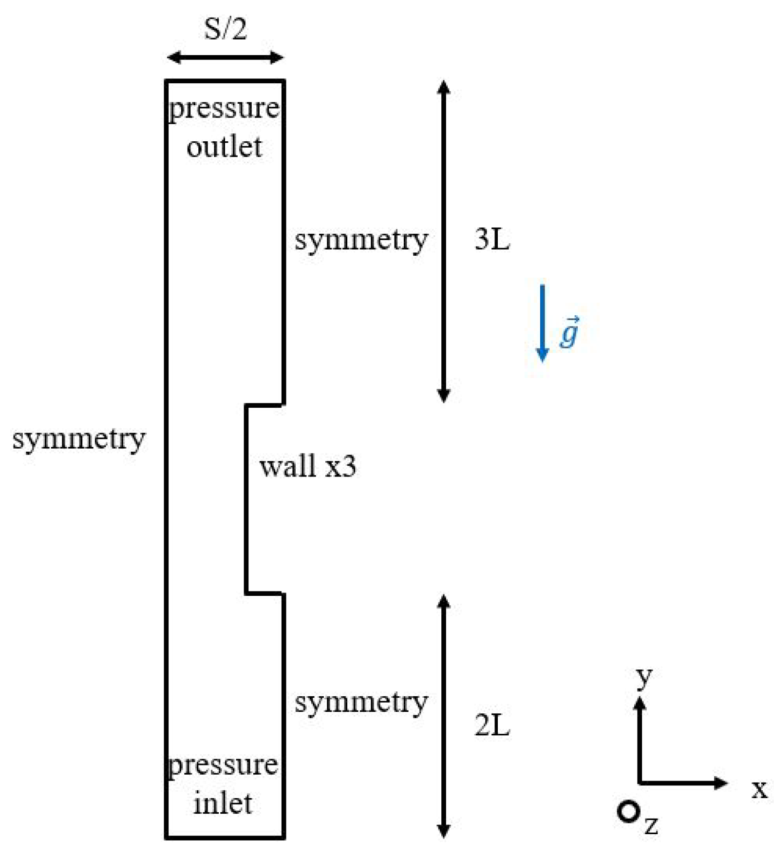
The boundary conditions for the 2D model were chosen as in Figure 2. Wall boundary conditions consisted of a no-slip isothermal wall. Imposed temperature was preferred over fixed heat flux, as this might lead to divergence especially for the 2D case given that the slice has no thickness. As already mentioned, in the quasi-3D case, the planes normal to the z direction are defined as periodic boundary conditions. Sometimes, for technical reasons which arise from the creation of periodic boundary conditions by Fluent, they were replaced by symmetry boundary conditions. Multiple tests were performed and this replacement has a negligible influence. For example, with

L = 1 m

S / 2 = 6 mm, Δ T = 60 K

, the difference between symmetry and periodic boundary conditions in the z direction was

0.8 %

. For the pressure inlet and outlet boundaries, a gauge pressure of

0 Pa

was chosen.

It is to be noted that, on simple models, comparison could be conducted against a 3D model. Obviously, it had a better correlation with semi-empirical formulas, typically less than

\pm 3 %

with Elenbaas’.

3. Results and Discussion

3.1. Parametric Study in 2D

In the first place, a parametric study was carried out in 2D, with the k-

ϵ

and laminar models. It used more than 60 design points, which were different combinations of the following parameters:

$L = 0.1 m, 0.5 m, 1 m, 1.5 m$ ,
$S / 2 = 2 mm, 6 mm, 10 mm, 15 mm, 20 mm, 50 mm$ ,
$Δ T = 60 K, 100 K, 300 K$ .

This allowing a large range of Elenbaas and Grashof numbers, more specifically:

E l \in [1, 3.42 \cdot 10^{7}]

and

G r_{L} \in [9.20 \cdot 10^{6}, 1.55 \cdot 10^{11}]

. Many points were also added in the intermediate region

10 ≲ E l ≲ 100

, which also coincides with

S / S_{o p t} \approx 1

This ensured that a wide variety of flows was covered, from fully laminar to mostly turbulent. The results for the k-

ϵ

model will be presented later, but many interesting conclusions can already be drawn from the results with the Fluent laminar model. It is to be noted it has been applied whatever the

G r_{L}

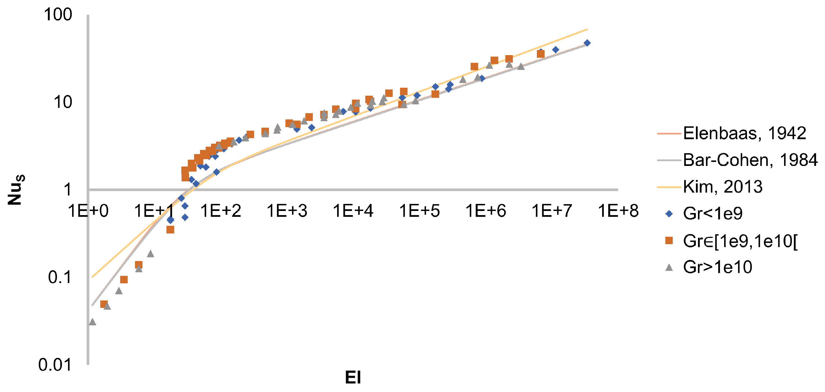
value was, so very likely some turbulent situations have been modelled with the laminar model. This is illustrated in Figure 3. Particular attention was paid to have many values for

G r_{L}

for all ranges of Elenbaas numbers. This is particularly relevant as it allows to uncorrelate those variables.

The Elenbaas semi-empirical correlation is valid up to

E l \approx 10^{7}

at least, whereas the current upper limit that had previously been tested was

10^{5}

[4].

However, at high Grashof number, the laminar model only dissipates heat through viscous effects, since the Kolmogorov cascade is not considered. Interestingly, the main region of difference between the current data points and the correlation is in the range where it is supposed to be the most precise, i.e., the intermediate region

10 ≲ E l ≲ 100

. The number of data points in that region seem to corroborate the fact that the semi-empirical correlations might be inaccurate in that domain, and the deviation is all the more important for

G r_{L} ≳ 10^{9}

. This is because the correlation is not used in its valid range for most points in that range. In other words, the laminar model is forcing the modelling of turbulent flows as laminar. This proves that the semi-empirical correlations are not valid for turbulent flows as stated earlier.

Also, this discrepancy could be the result of inaccurate predictions regarding asymptotic behaviours. Typically, the Bar-Cohen correlation assumes two asymptotic behaviours as mentioned earlier, but unfortunately, the region where the relation is supposed to be the most accurate, typically

10 ≲ E l ≲ 100

, is also where the two asymptotic behaviours intersect, thus leading to high deviations, as the merging process, corresponding to the exponent

- 1 / 2

, has no physical meaning but is only a statistical modelling.

3.2. New Grouping Factors: Examining Physical Parameters Governing Heat Sink Performance

One of the major goals of this work is also to find grouping factors. Grouping factors are physical quantities that dictate the overall behaviour of the system, with respect to semi-empirical correlations. If possible, those quantities should be dimensionless so that they can be easily transposed to any geometry. In that sense, they could also be named scaling factors. However, further research would be needed to prove that they are indeed independent of the size and shape of the heat sink. The Elenbaas number is a clear example of grouping factor for this problem as all the correlations from Section 1.1 are of the form

\bar{N u_{S}} = f (E l)

The first strategy to find other grouping factors is to group data points by value of external parameters which are not directly related to the Elenbaas number itself, as depicted in Figure 3:

G r_{L}

is not a grouping factor. Conversely,

S / S_{o p t}

stands out as an appropriate one. As a reminder,

S_{o p t}

is here defined as the optimal grouping factor according to Bar-Cohen’s correlation, as in Equation 5.

S / S_{o p t}

is consequently an intricate function of the physical and geometrical parameters of the problem, i.e.,

L, S

and

Δ T

, as

R a_{L}

itself depends on L and

Δ T

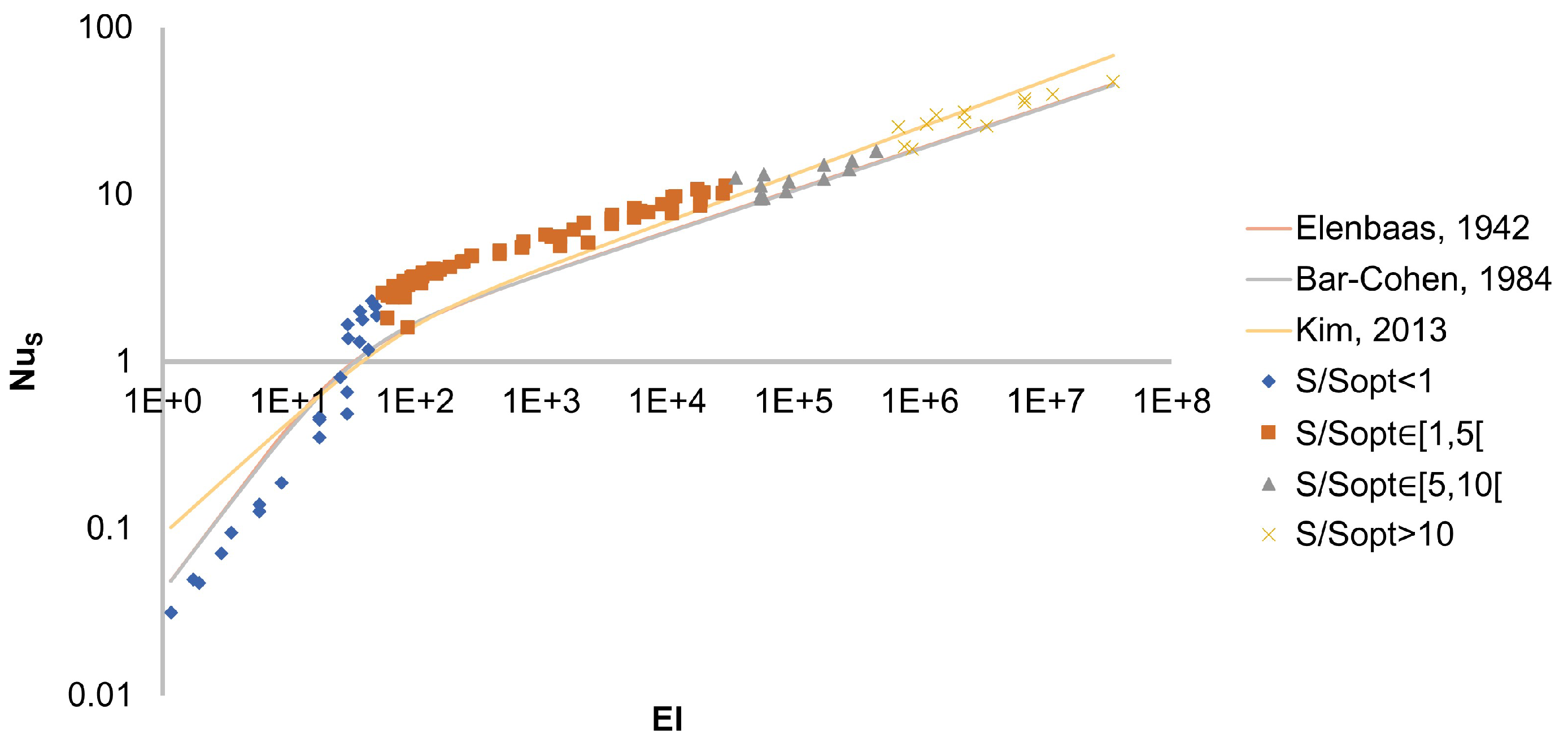
. Figure 4 clearly shows that for

S / S_{o p t}

slightly under 1, the current data points would switch between both asymptotic behaviours.

S / S_{o p t}

stands out as the best way to normalize S, and the following physical interpretations can be given, which were backed up by numerical simulations:

$S / S_{o p t} ≲ 1$ : the boundary layers of two adjacent fins are deeply merging, thus corresponding to the low $E l$ behaviour,
$S / S_{o p t} ≳ 1$ : the fins can, up to some extent, be considered as isolated, that is the high $E l$ behaviour.

3.3. Comparison with Churchill and Chu’s Correlation

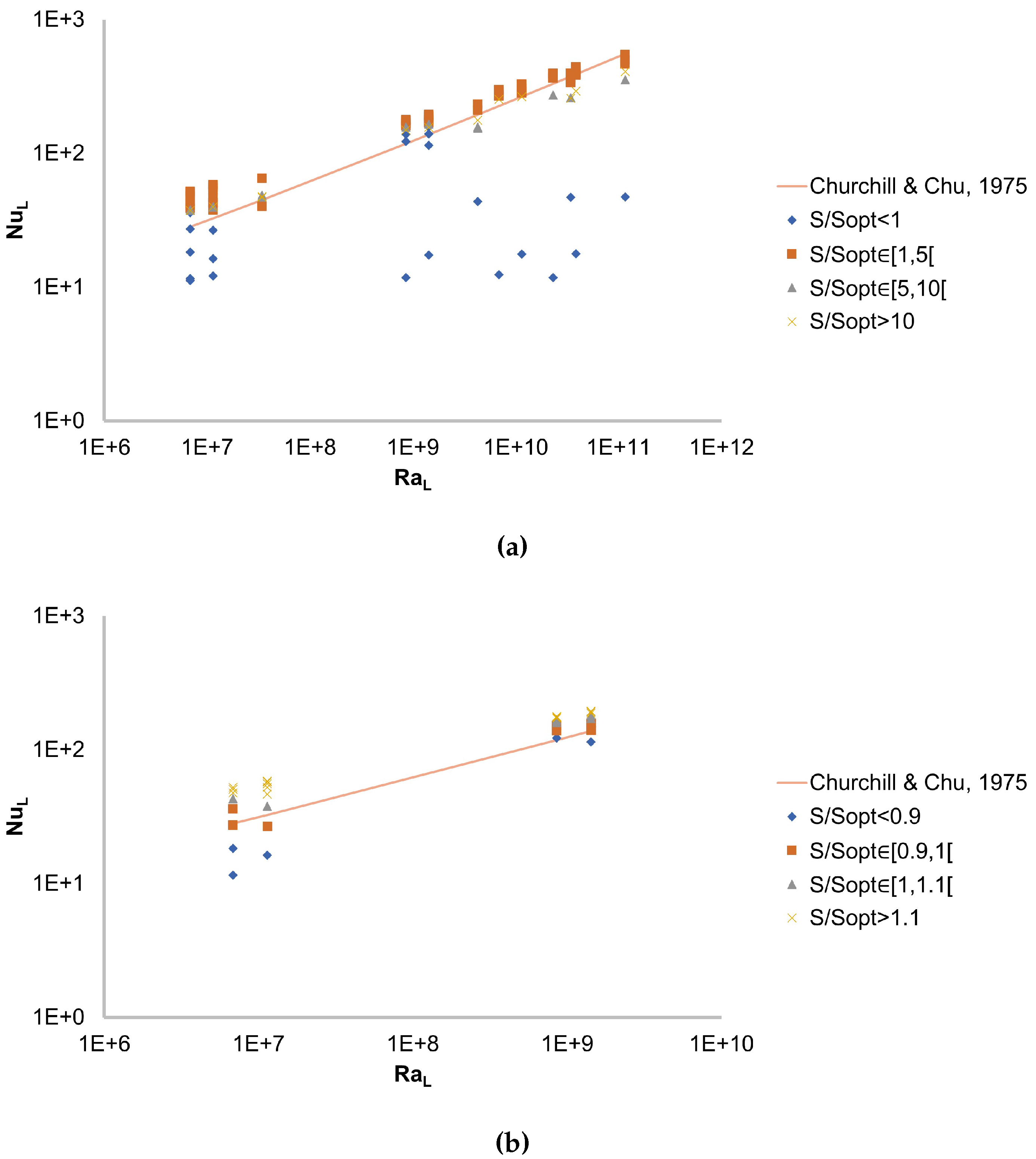
Another means of validation of the data would be to compare it with Churchill and Chu’s correlation. This correlation is valid for natural convection for vertical plates, so it does not properly apply to an array of fins. However, it is valid for a much wider range of flows compared to the other correlations before, namely

10^{4} ≲ R a_{L} ≲ 10^{13}

, and in particular can account for turbulent flows. Obviously, S is not a parameter for this correlation, which is why it will be plotted in a different manner than for Figure 3 and Figure 4, and it reads [4,23]:

\bar{N u_{L}} = {(0.825 + \frac{0.387 R a_{L}^{1 / 6}}{{[1 + {(0.492 / P r)}^{9 / 16}]}^{8 / 27}})}^{2}

(7)

As a consequence, the data points from the 2D Fluent laminar model can be plotted in a graph

(R a_{L}, \bar{N u_{L}})

and be compared with Churchill and Chu’s relation, as in Figure 5. This graph is interesting in the sense that it validates our model for large values of S, typically larger than

S_{o p t}

: the values have a small deviation from the correlation. It also means that Churchill and Chu’s correlation is applicable for large spacings to find the total heat transfer coefficient from

\bar{N u_{L}}

, and that although the other correlations are valid in those cases, they are not necessary [23]. Finally, it also confirms that

S / S_{o p t}

is a grouping factor for natural convection heat sink applications.

In order to precisely find the threshold for

S / S_{o p t}

, a more detailed study was performed with values of

S / S_{o p t}

around 1 as this was mentioned before. Most values for

S / S_{o p t}

ranged between

0.8

and

1.2

, hence the rescaling for the values of

S / S_{o p t}

represented in Figure 5. It indeed shows that the threshold between both behaviours occurs at exactly

S / S_{o p t} = 1

, and also that this transition is less sharp for low Rayleigh numbers.

As mentioned earlier, the 2D model is not really adapted for turbulence modelling. Indeed, turbulence is inherently a 3D model [4,20], which is why the transition-SST led to very poor performance on the 2D model. The k-

ϵ

models yielded somehow better results, but still not acceptable when compared to the correlations. This is why a similar parametric study was conducted with the quasi-3D model.

3.4. Parametric Study in Quasi-3D

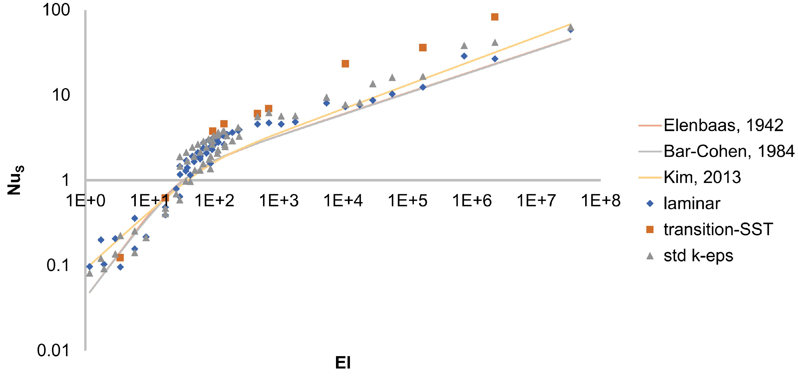
In this section, the simulations were carried out using the quasi-3D model, also referred to as periodic model. Once again, special attention was paid to have all kinds of flows i.e., a wide range of

G r_{L}

in every Elenbaas number regions.

The comparison will be made, between the Fluent laminar, transition-SST and standard k-

ϵ

models. Results are presented in Figure 6. Once again, good correlation is observed between theoretical correlations and the current CFD data, which validates the models.

The transition-SST model has fewer points than the other two. This is because it has to be initialized from a converged laminar case, thus making direct parametric studies harder to conduct and extremely long to converge without proper initialization.

Turbulence is known to enhance heat transfer, as it can be theoretically predicted [4], or by numerical simulations [10,21]. Then, it seems logical that the value predicted by the transition-SST model lies between the laminar and the other turbulence models, as it is known to accurately take into account the transition zone between both regimes. Furthermore, the k-

ϵ

model is known to have relatively poor performance in the near-wall region i.e., in the boundary layers. This is why its value is the most extreme and the furthest from the predictions of semi-empirical correlations.

However, this order is not true for high

E l

, typically greater than

10^{4}

. As a consequence, the transition-SST model should not be used in that range. It can also be confirmed for a wider range of Elenbaas numbers that the k-

ϵ

model over-estimates the heat flux with respect to the laminar model: this is a well-known consequence of turbulence models. Overall all those conclusions are consistent with what was observed so far, and also in the literature [10,21]. In summary:

The laminar model provides good estimations of the heat flux whatever the operating conditions: for instance, it is not dependant on the value of $G r_{L}$ . 2D simulations are sufficient for the laminar model, but it is the only model for which this is true.
The transition-SST model is deemed to be the most accurate for $E l ≲ 10^{4}$ , which indeed seems consistent as it was especially developed for this kind of applications.
The k- $ϵ$ model tends to over-estimate the heat flux over the whole range of Elenbaas numbers. Consequently, it should be used with precaution, although it gives a good estimation of the heat flux in a shorter delay as the mesh can be coarser thanks to the usage of wall functions, notably Enhanced Wall Treatment (EWT). Also, the deviation for average values of the y velocity from the laminar model was the highest, which might mean poorer prediction regarding the flow equations.

The same methodology as in Section 3.2 was applied with the quasi-3D results, with similar results.

S / S_{o p t}

was also found to be an appropriate factor with a very clear threshold at 1, whatever the Fluent model. This acted again as a validation of the model, and confirmed once again

S / S_{o p t}

as an important parameter regarding the simulation strategy.

The turbulent models themselves should be accurately validated, to fit them to general simulations in natural convection, without even considering the correlations aforementioned. For instance, LES (Large Eddy Simulation) models could be used for this purpose.

3.5. Influence of the Number of Cells in the z Direction

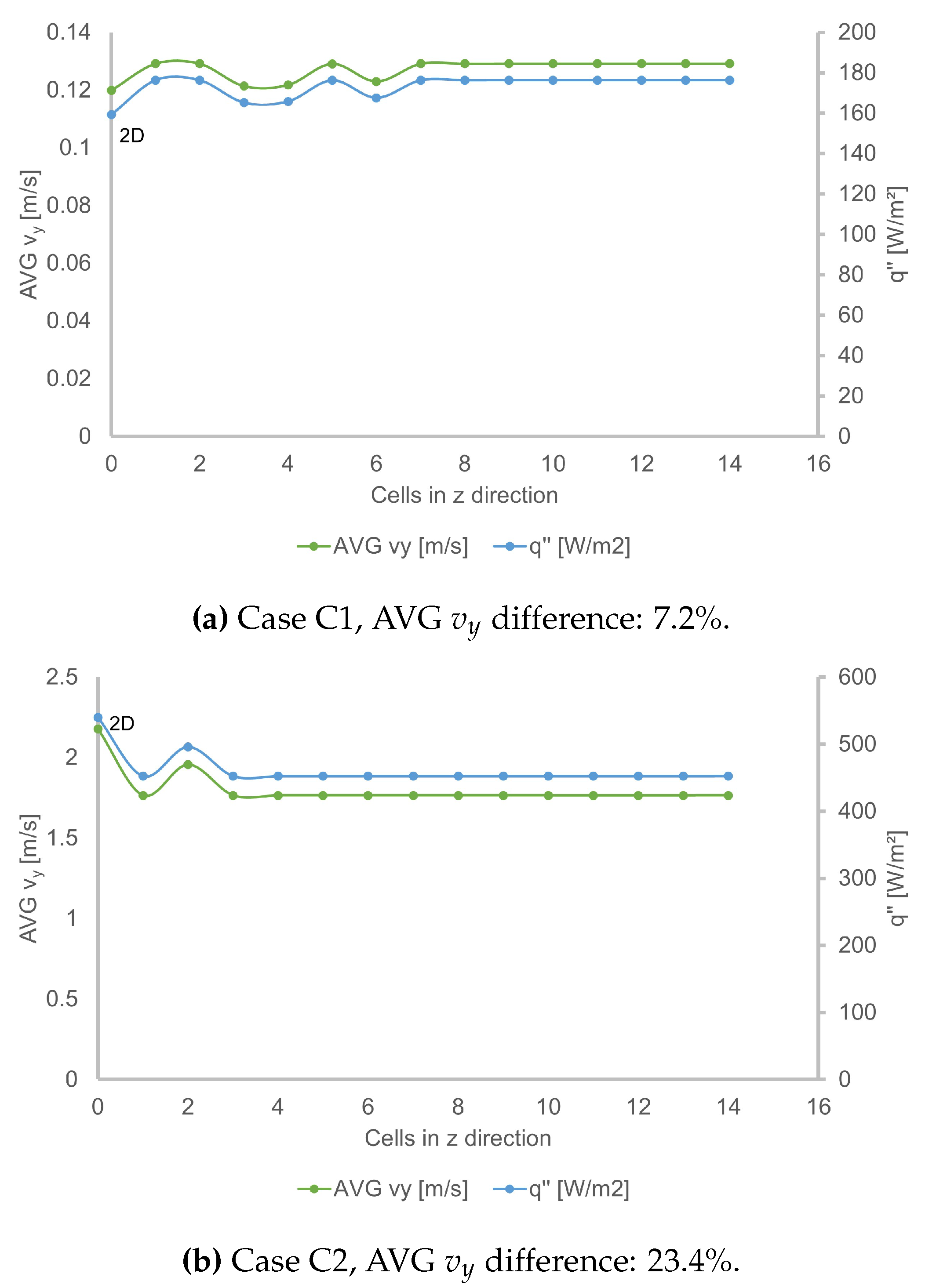
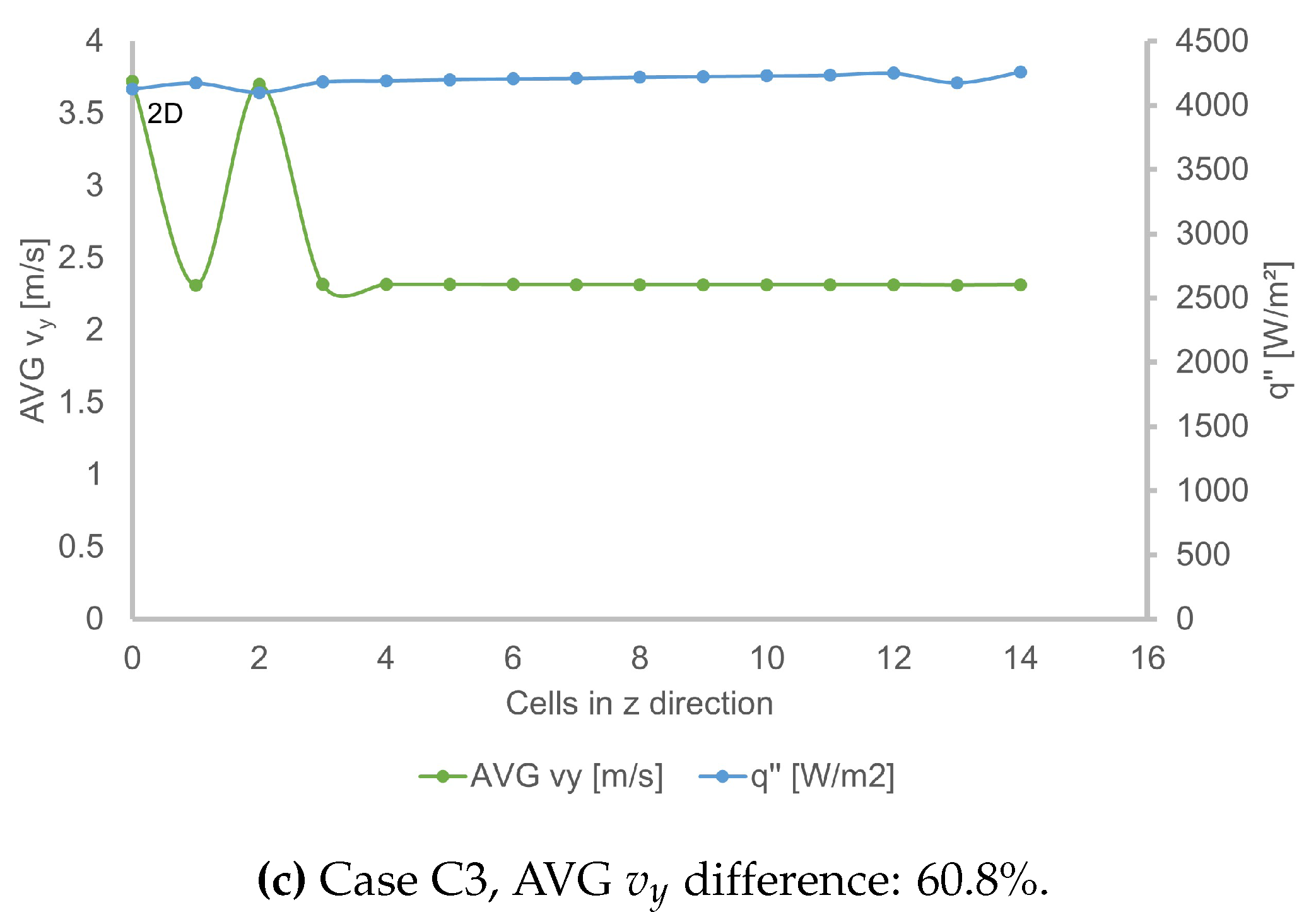
The k-

ϵ

model provides significantly different results when comparing 2D with quasi-3D models. As a consequence, a study was conducted on the number of cells in the z direction, only for this model as the results were more blatant. As a reminder, the z direction is the direction normal to the periodic boundary condition planes. A higher number of cells in the z direction should mean better prediction, but also increases the number of cells in a linear way as the mesh is fully structured.

Three design points were chosen at low, medium and high Elenbaas numbers: cases C1, C2 and C3, and the number of cells varied from 1 to 14.

C1.: $L = 0.1 m$ , $S / 2 = 2 mm$ , $Δ T = 60 K$ , $E l = 17$ , $G r_{L} = 9.20 \cdot 10^{6}$
C2: $L = 1.5 m$ , $S / 2 = 6 mm$ , $Δ T = 60 K$ , $E l = 95$ , $G r_{L} = 3.10 \cdot 10^{10}$
C3: $L = 1.5 m$ , $S / 2 = 50 mm$ , $Δ T = 300 K$ , $E l = 2.28 \cdot 10^{6}$ , $G r_{L} = 1.55 \cdot 10^{11}$

If that number equals zero it means that the 2D result is considered. As usual, the average values of

v_{y}

and

q^{''}

are presented on two separate scales in Figure . For a small number of cells, typically less than 4, there are significant variations in the results provided by the models. The predictions deviate more from the correlations for low Elenbaas numbers (C1), as this has been shown before: it is thus recommended to have more than 10 cells in the z direction for those cases. This also explains why the 2D model is not well adapted for k-

ϵ

simulations, and should be linked with the previous subsection.

There is also a higher discrepancy between 2D and 3D results for high Grashof numbers, and this has also been verified in the literature [21] and with other design points in this study. Typically, the difference between 2D and 3D results regarding the average velocity

v_{y}

is given in each caption (Figure ). This error increases with

G r_{L}

, corroborating the fact that the 2D model cannot capture highly turbulent effects. For such applications, the quasi-3D model is recommended.

4. Conclusions

This work focused on providing an efficient and accurate strategy to simulate buoyancy-driven flows around heat sinks. Plate-fin heat sinks were mostly studied, as they are the only ones for which several semi-empirical correlations were developed.

The 2D model over-estimates the heat flux by approximately 10 to

20 %

compared to the Elenbaas correlation, but is obviously less computationally demanding. It is recommended to use only the laminar model on the 2D model, as any turbulent model will result to high deviation with the correlation. The laminar model also proved wrong for high Grashof numbers as could intuitively be predicted: turbulent models must absolutely be used in such cases. It was also found that the Elenbaas correlation is in reality valid up to

E l \approx 10^{7}

at least. Elenbaas numbers up to

3.42 \cdot 10^{7}

and Grashof numbers up to

1.55 \cdot 10^{11}

were simulated.

The quasi-3D model will provide the best results, and proved to be a very good trade-off between quality and computational time. With the Fluent laminar model, the results were very close to the 2D case, but this model had a smaller deviation for the transition-SST and k-

ϵ

models. It was found that the k-

ϵ

model provided relatively good results with a coarser mesh for any Elenbaas number. For low and medium Elenbaas numbers, the transition-SST model provides the most consistent results, but it should be avoided for high Elenbaas numbers.

Author Contributions

Conceptualization, L.D., R.N., S.M.A. and T.P.; methodology, L.D., R.N., S.M.A. and T.P.; software, L.D., R.N. and S.M.A.; validation, L.D.; formal analysis, L.D.; investigation, L.D.; resources, T.P.; data curation, L.D.; writing—original draft preparation, L.D.; writing—review and editing, R.N., S.M.A and T.P.; visualization, L.D.; supervision, R.N., S.M.A and T.P.; project administration, R.N., S.M.A and T.P. All authors have read and agreed to the published version of the manuscript.

Funding

This research received no external funding.

Data Availability Statement

The data presented in this study are available upon request from the corresponding author.

Conflicts of Interest

The authors declare no conflicts of interest.

Nomenclature

A	Area of contact	$m^{2}$
$E l$	Elenbaas number	$-$
$G r$	Grashof number	$-$
H	Height of the fin	$m$
L	Length of the fin	$m$
$N u$	Nusselt number	$-$
$R a$	Rayleigh number	$-$
$R_{t h}$	Thermal resistance	$K / W$
S	Spacing between two adjacent fins	$m$
Q	Total heat power	$W$
g	Standard acceleration of gravity	$m / s^{2}$
h	Convective heat transfer coefficient	$W / (m^{2} K)$
k	Thermal conductivity	$W / (mK)$
$q^{''}$	Heat dissipation per unit area	$W / m^{2}$
t	Thickness of a fin	$m$
$Δ T$	Temperature difference	$K$
$β$	Volumetric thermal expansion coefficient	$/ K$

Abbreviations

The following abbreviations are used in this manuscript:

CFD	Computational fluid dynamics
EWT	Enhanced Wall Treatment
HTC	Heat transfer coefficient
SST	Shear-stress transport (model)

References

Balaji, C.; Srinivasan, B.; Gedupudi, S. Heat Transfer Engineering: Fundamentals and Techniques; Elsevier Science: Amsterdam, Netherlands, 2020. [Google Scholar]
Zhang, Z.; Wang, X.; Yan, Y. A review of the state-of-the-art in electronic cooling. e-Prime - Advances in Electrical Engineering, Electronics and Energy 2021, 1, 100009. [Google Scholar] [CrossRef]
Elenbaas, W. Heat dissipation of parallel plates by free convection. Physica 1942, 9, 1–28. [Google Scholar] [CrossRef]
Bergman, T.L.; Lavine, A.S.; Incropera, F.P.; Dewitt, D.P. Fundamentals of heat and mass transfer, 7th ed ed.; Wiley: Hoboken, NJ, USA, 2011. [Google Scholar]
Bar-Cohen, A.; Rohsenow, W.M. Thermally Optimum Spacing of Vertical, Natural Convection Cooled, Parallel Plates. Journal of Heat Transfer 1984, 106, 116–123. [Google Scholar] [CrossRef]
Van De Pol, D.W.; Tierney, J. Free Convection Heat Transfer from Vertical Fin-Arrays. IEEE Transactions on Parts, Hybrids, and Packaging 1974, 10, 267–271. [Google Scholar] [CrossRef]
Kim, T.H.; Kim, D.K.; Do, K.H. Correlation for the fin Nusselt number of natural convective heat sinks with vertically oriented plate-fins. Heat and Mass Transfer 2013, 49, 413–425. [Google Scholar] [CrossRef]
Wong, S.C.; Chu, S.H. Revisit on natural convection from vertical isothermal plate arrays–effects of extra plume buoyancy. International Journal of Thermal Sciences 2017, 120, 263–272. [Google Scholar] [CrossRef]
Fan, Y.; Zhao, Y.; Torres, J.F.; Xu, F.; Lei, C.; Li, Y.; Carmeliet, J. Natural convection over vertical and horizontal heated flat surfaces: A review of recent progress focusing on underpinnings and implications for heat transfer and environmental applications. Physics of Fluids 2021, 33, 101301. [Google Scholar] [CrossRef]
McCay, O.; Nimmagadda, R.; Ali, S.M.; Persoons, T. A Parametric Design Study of Natural-Convection-Cooled Heat Sinks. Fluids 2023, 8, 234. [Google Scholar] [CrossRef]
Bar-Cohen, A.; Iyengar, M.; Kraus, A.D. Design of Optimum Plate-Fin Natural Convective Heat Sinks. Journal of Electronic Packaging 2003, 125, 208–216. [Google Scholar] [CrossRef]
Abbas, A.; Wang, C.C. Augmentation of natural convection heat sink via using displacement design. International Journal of Heat and Mass Transfer 2020, 154, 119757. [Google Scholar] [CrossRef]
Feng, S.; Shi, M.; Yan, H.; Sun, S.; Li, F.; Lu, T.J. Natural convection in a cross-fin heat sink. Applied Thermal Engineering 2018, 132, 30–37. [Google Scholar] [CrossRef]
Chang, S.W.; Wu, H.W.; Guo, D.Y.; Shi, J.j.; Chen, T.H. Heat transfer enhancement of vertical dimpled fin array in natural convection. International Journal of Heat and Mass Transfer 2017, 106, 781–792. [Google Scholar] [CrossRef]
Ray, R.; Mohanty, A.; Patro, P.; Tripathy, K.C. Performance enhancement of heat sink with branched and interrupted fins. International Communications in Heat and Mass Transfer 2022, 133, 105945. [Google Scholar] [CrossRef]
Zhang, K.; Li, M.J.; Wang, F.L.; He, Y.L. Experimental and numerical investigation of natural convection heat transfer of W-type fin arrays. International Journal of Heat and Mass Transfer 2020, 152, 119315. [Google Scholar] [CrossRef]
Ma, H.; He, L. Large eddy simulation of natural convection heat transfer and fluid flow around a horizontal cylinder. International Journal of Thermal Sciences 2021, 162, 106789. [Google Scholar] [CrossRef]
Murphy, P. Characterisation of the Flow and Heat Behaviour Associated with a Wall-Bounded Dual Jet Flow. PhD thesis, Trinity College Dublin, Dublin, Ireland, 2024.
Alimohammadi, S.; Murray, D.B.; Persoons, T. Experimental Validation of a Computational Fluid Dynamics Methodology for Transitional Flow Heat Transfer Characteristics of a Steady Impinging Jet. Journal of Heat Transfer 2014, 136, 091703. [Google Scholar] [CrossRef]
Ansys Inc. ANSYS Fluent Theory Guide.
Lee, J.R. On the three-dimensional effect for natural convection in horizontal enclosure with an adiabatic body: Review from the 2D results and visualization of 3D flow structure. International Communications in Heat and Mass Transfer 2018, 92, 31–38. [Google Scholar] [CrossRef]
Roache, P.J. Perspective: A Method for Uniform Reporting of Grid Refinement Studies. Journal of Fluids Engineering 1994, 116, 405–413. [Google Scholar] [CrossRef]
Churchill, S.W.; Chu, H.H. Correlating equations for laminar and turbulent free convection from a vertical plate. International Journal of Heat and Mass Transfer 1975, 18, 1323–1329. [Google Scholar] [CrossRef]

Figure 1. Definition of the dimensions and of the three geometrical models. Not shown to scale. Gravity is in the downward y direction.

Figure 2. Definition of the boundary conditions for the 2D model.

Figure 3. Comparison of 2D Fluent laminar results with theoretical correlations [3,5,7], with data grouped by values of

G r_{L}

Figure 3. Comparison of 2D Fluent laminar results with theoretical correlations [3,5,7], with data grouped by values of

G r_{L}

Figure 4. Comparison of 2D Fluent laminar results with theoretical correlations [3,5,7], with

S / S_{o p t}

as a grouping factor.

Figure 4. Comparison of 2D Fluent laminar results with theoretical correlations [3,5,7], with

S / S_{o p t}

as a grouping factor.

Figure 5. Comparison of 2D Fluent laminar results with Churchill and Chu’s relation [23], with data grouped by values of

S / S_{o p t}

, with (a) large scaling, (b) detailed scaling around 1.

Figure 5. Comparison of 2D Fluent laminar results with Churchill and Chu’s relation [23], with data grouped by values of

S / S_{o p t}

, with (a) large scaling, (b) detailed scaling around 1.

Figure 6. Comparison between Fluent models for the quasi-3D model, along with theoretical correlations [3,5,7].

Figure 7. Influence of the number of cells in the z direction.

Table 1. Ranges of values for geometrical and physical parameters.

Description	Symbol	Value	Unit
Vertical length	L	$0.1 - - - 1.5$	$m$
Half-spacing (width)	$S / 2$	$2 - - - 50$	$mm$
Temperature difference $T_{s} - T_{\infty}$	$Δ T$	$60 - - - 300$	$K$
Elenbaas number	$E l$	$1.17 - - - 3.42 \cdot 10^{7}$	$-$
Grashof number	$G r_{L}$	$9.22 \cdot 10^{6} - - - 1.55 \cdot 10^{11}$	$-$

Table 2. Material properties.

Description	Symbol	Value	Unit
Dynamic viscosity	$μ$	$1.79 \cdot 10^{- 5}$	$kg / m / s$
Density (Boussinesq approximation)	$ρ_{0}$	$1.225$	$kg / m^{3}$
Thermal conductivity	k	$0.0242$	$W / m / K$
Specific heat capacity	$C_{p}$	$1006.43$	$J / kg / K$
Thermal diffusivity	a	$1.963 \cdot 10^{- 5}$	$m^{2} / s$
Prandtl number	$P r$	0.744	$-$

Disclaimer/Publisher’s Note: The statements, opinions and data contained in all publications are solely those of the individual author(s) and contributor(s) and not of MDPI and/or the editor(s). MDPI and/or the editor(s) disclaim responsibility for any injury to people or property resulting from any ideas, methods, instructions or products referred to in the content.

© 2024 by the authors. Licensee MDPI, Basel, Switzerland. This article is an open access article distributed under the terms and conditions of the Creative Commons Attribution (CC BY) license (http://creativecommons.org/licenses/by/4.0/).

Copyright: This open access article is published under a Creative Commons CC BY 4.0 license, which permit the free download, distribution, and reuse, provided that the author and preprint are cited in any reuse.

MDPI Initiatives

Important Links

Choose an area of interest and we will send you notifications of new preprints at your preferred frequency.

Disclaimer