3.1. Software Features
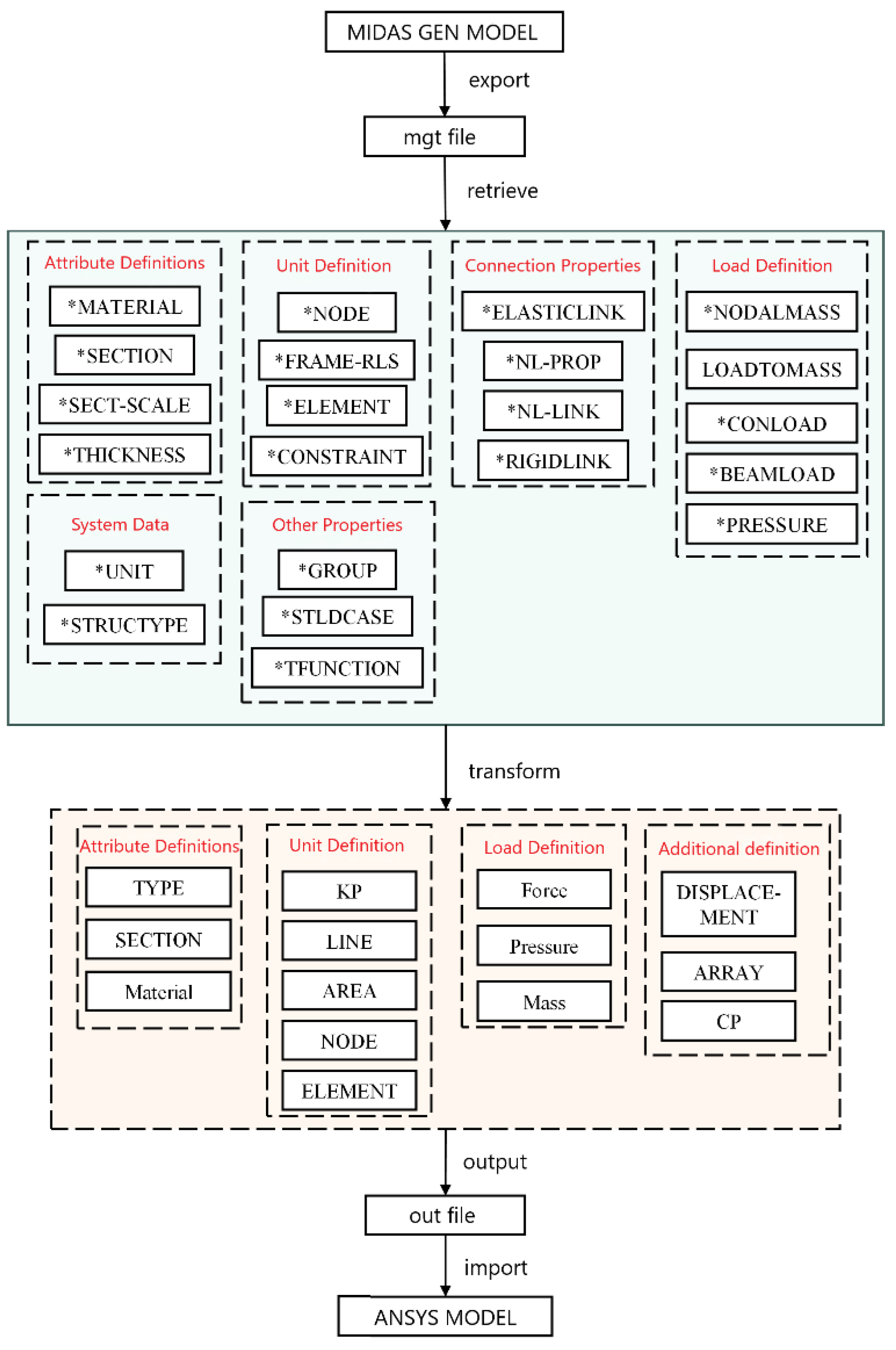
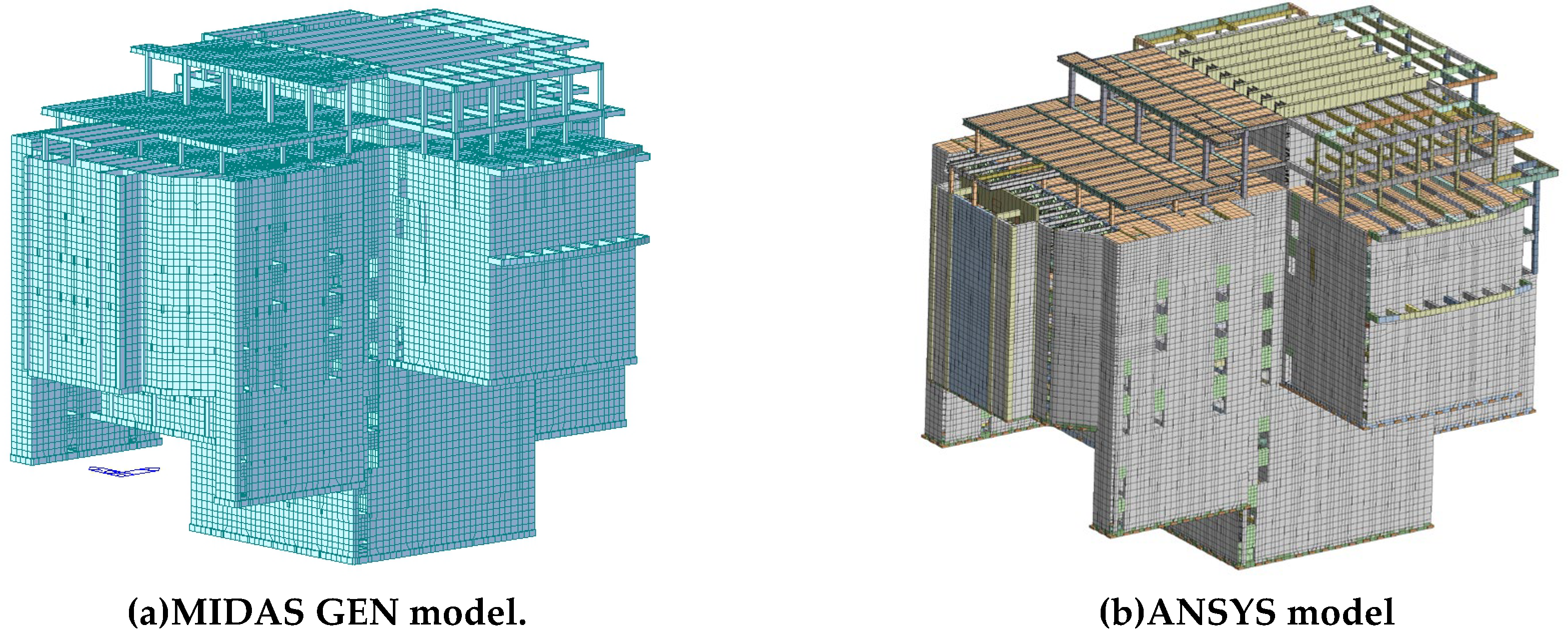
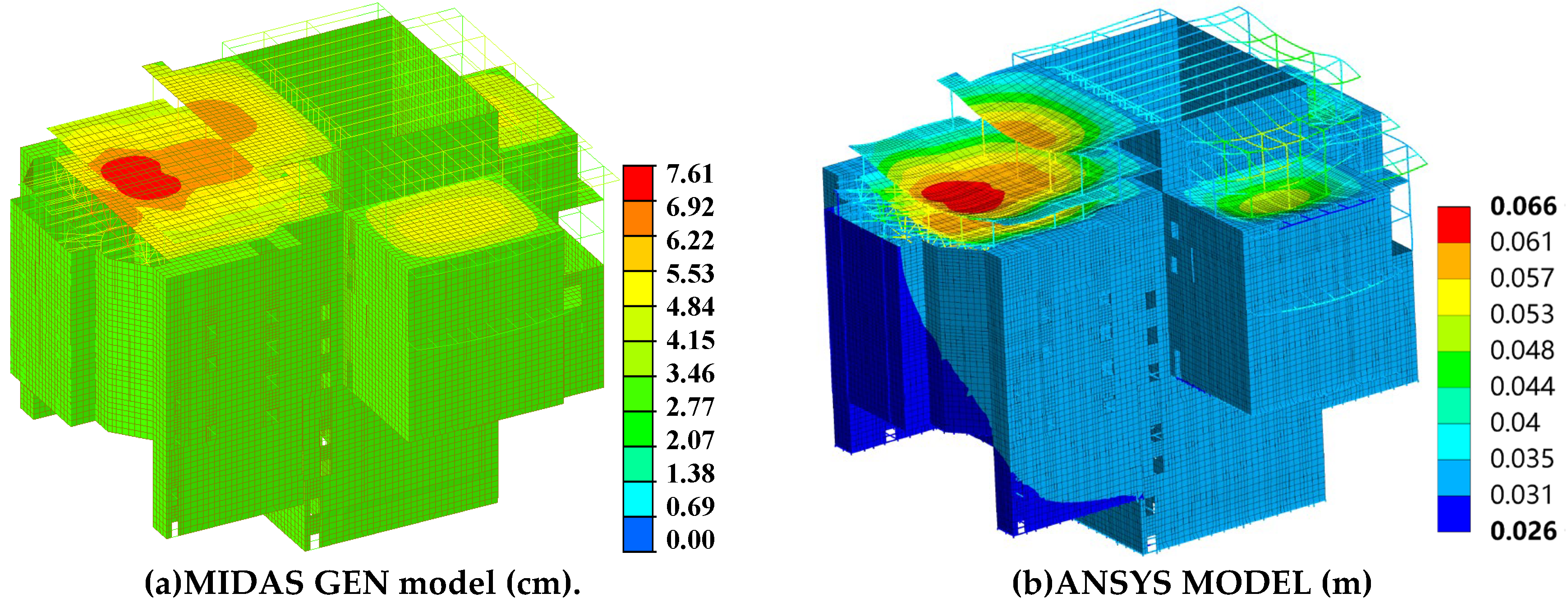
The conversion program is capable of importing and reading the MDIAS GEN data file. By analyzing, processing and integrating the program data, the APDL command streams out a file that ANSYS can read is exported, thereby enabling the rapid modeling of ANSYS. The specific conversion functions are as follows:
(1) The structural properties include the material, section, section parameter scaling, wall thickness and so on. For some special sections, such as national standard hot rolled section steel or custom sections, manual input is required and automatic conversion cannot be achieved.
(2) The nodes in MIDAS are converted to the key points in ANSYS, resulting in a one-to-one correspondence between the two. The beam-plate element is converted into a line and area in ANSYS. The program automatically selects the corresponding element type. Generally, the BEAM188 element is used for the beam and column, while the SHELL181 element is used for the wall and plate. The mesh size of each unit can be modified according to the user’s specifications. The key points, lines and surfaces can be further divided into finite element meshes.
(3) Special element transformations, such as node mass, elastic connection element, general connection element, etc. The mass of the joint is simulated by the MASS21 element in ANSYS, and the elastic connection element uses the COMBIN14 element. However, the elastic connection unit and the general connection unit play different roles in MIDAS and possess a multitude of functions. Therefore, it is imperative to correspond to different unit settings according to the attributes of the different units.
(4) Setting the release beam end constraint in MDIAS GEN to realize the hinge of the beam and column. Creating the rigid domain can also be converted to the ANSYS model through the program.
(5) The transformation of a variety of load conditions, such as node load, beam-column distribution load, plate and shell uniform load, etc. A variety of working conditions need to be grouped and converted to generate different models or simple load files.
(6) Time history function conversion is also a function. ARRAY is used to store time history data in ANSYS. For different time history waves or vibration waves, multiple ARRAYs can be used for storage and the time history wave can be pre-scaled by setting the scaling coefficient.
3.2. Key Issues Addressed
(1) Line unit 3 axis direction
In ANSYS, the line element (BEAM188) must be defined with specific key points to determine the 3-axis direction of the section. In MIDAS, there is a corresponding element angle corresponding to it and the 3-axis direction can be adjusted. The three-axis direction determination rules of the two are the same, but there is only a component β angle in MIDAS GEN [
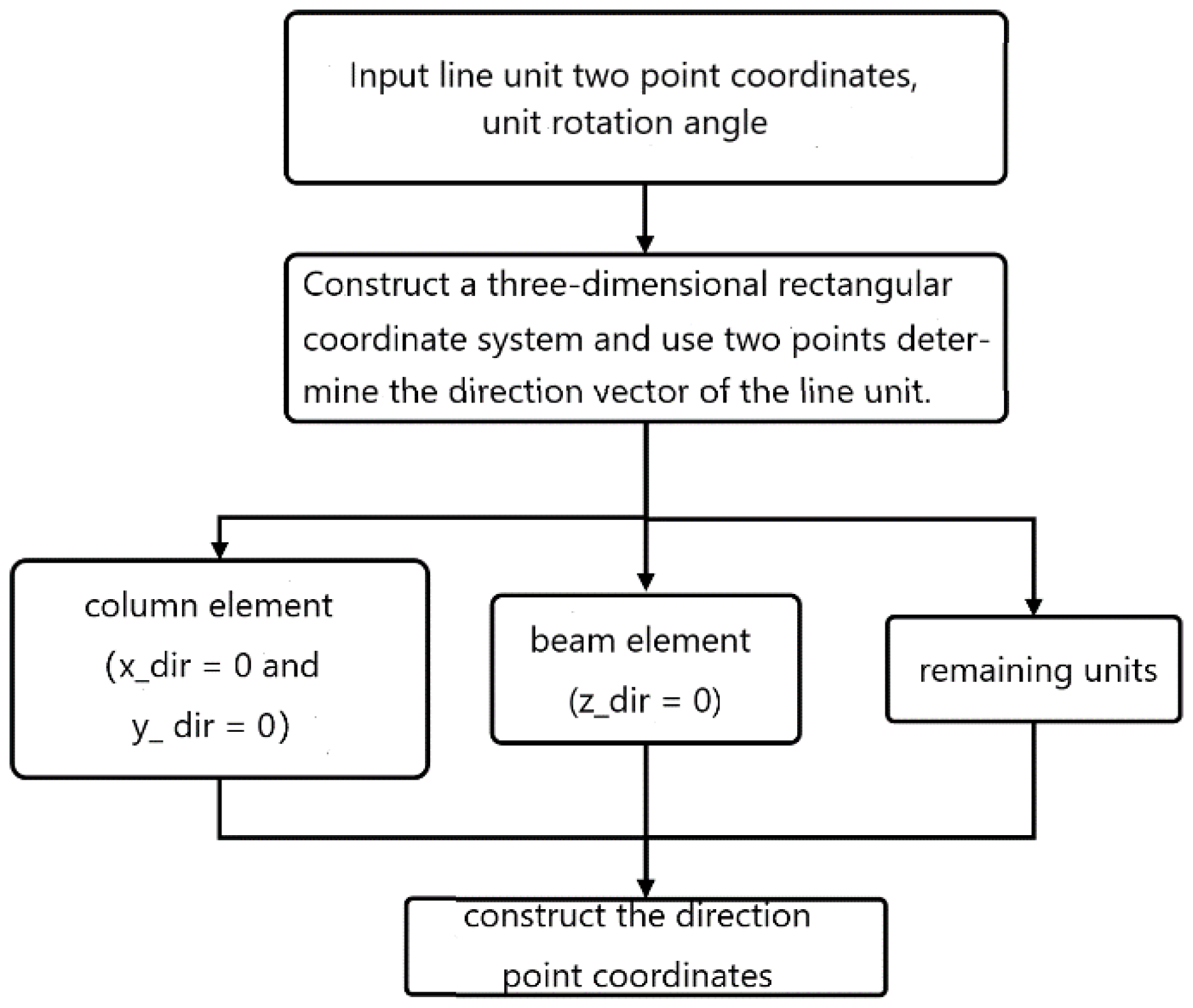
17]. In ANSYS, the data must be converted into a unit direction point, which requires further construction. The direction point construction process is shown in
Figure 7.
In the above steps, x_dir, y_dir and z_dir are the three coordinate values of the direction vector of the line element respectively. If x_dir = 0 and y_dir = 0, the direction vector is perpendicular to the Z axis and is identified as a cylindrical element. The z_dir = 0 indicates that the direction vector is parallel to the XY plane and is identified as a beam element. After the classification of the unit, it is more important to find the vector corresponding to the zero rotation angle of the line unit, which means to find a vertical line through the line unit in the plane (OXY plane, OXZ plane, OYZ plane )where the line unit is located. Finally, the final direction vector and direction key points are determined according to different rotation angles. The method for calculating the direction point vector is given below. Vector1, Vector2 and Angle are the line unit direction vector, the vertical vector of the line unit direction vector and the unit rotation angle [
18] respectively.
| Algorithm 1: getAngleVector |
Input: vector1: a three-dimensional vector in space [x1, y1, z1], vector2: a three-dimensional vector in space [x2, y2, z2], angle: target angle (in radians) between the resulting vector and vector2
1. If length(vector1) = 3 or length(vector2) = 3
2. Calculate dot_product = vector1[0]*vector2[0] + vector1[1]*vector2[1] + vector1[2]*vector2[2]
3. Calculate product_length = sqrt((vector1[0]**2 + vector1[1]**2 + vector1[2]**2) * (vector2[0]**2 + vector2[1]**2 + vector2[2]**2))
4. Calculate cos_angle = dot_product / product_length
5. Calculate delta_angle = angle - acos(cos_angle)
6. Calculate new vector coordinates:
x = cos(delta_angle)*vector2[0] + sin(delta_angle)*vector1[0]
y = cos(delta_angle)*vector2[1] + sin(delta_angle)*vector1[1]
z = cos(delta_angle)*vector2[2] + sin(delta_angle)*vector1[2]
7. Find max_ = max(abs(x), abs(y), abs(z))
8. Normalize vector coordinates:
x’ = x / max_
y’ = y / max_
z’ = z / max_
9. Return result_vector = [x’, y’, z’]
10. Else if return None
11. End if
12. End |
(2) Rigid domain problem
In structural modeling, some short beams and short columns are used to connect two components, which are often replaced by rigid rods in software. At the same time, in the process of grid division of plate wall elements, there will also be some elements with very small areas or extremely irregular shapes. The size of these line and surface elements is very small compared with other elements, which will greatly affect the calculation speed of the software. Especially when the display dynamics analysis is carried out in LS-DYNA, the minimum element size is directly related to the software calculation speed [
19,
20]. To reduce its influence, the above unit can be set as a rigid unit in the ANSYS modeling process, which means that the material property is set to be rigid.
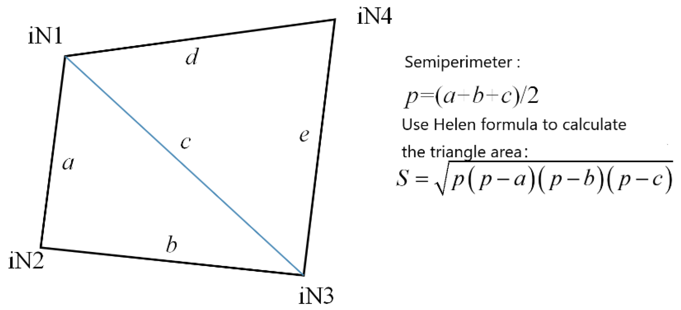
For the line element, the distance between the two nodes is calculated as the length of the line element. And the length of the line element is less than the limit value, which can be set as the rigid element. For the surface element, the area less than the limit is set as the rigid element. In addition, some units with extremely irregular shapes, are also set as rigid units, such as a large aspect ratio and a very small angle between the edges. The above units are determined by the ratio of the area to the square of the longest diagonal.
However, if two minimal elements contain common nodes, they cannot be set as two independent rigid elements. Therefore, it is necessary to combine these two independent rigid elements into one rigid element, which means setting the same rigid material properties. The above operation must iterate through all the rigid elements. Then find out the elements with common nodes for grouping and set the rigid material. A Python program is listed below that uses Helen’s formula to calculate the area of the specified four points (
Figure 8) and the ratio of the longest diagonal.
| Algorithm 2: CalculateAreaAndLengthRatio |
Input: iN1, iN2, iN3, iN4: coordinates of four points in 3D space (e.g., iN1 = [x1, y1, z1])
Output: BI: ratio of the area to the square of the longest diagonal; S: total area of the quadrilateral
1. Extract coordinates from input points:
x1, y1, z1 = iN1
x2, y2, z2 = iN2
x3, y3, z3 = iN3
x4, y4, z4 = iN4
2. Calculate edge lengths and diagonal lengths:
a = sqrt((x2-x1)**2 + (y2-y1)**2 + (z2-z1)**2) // Length of edge between N1 and N2
b = sqrt((x3-x2)**2 + (y3-y2)**2 + (z3-z2)**2) // Length of edge between N2 and N3
c = sqrt((x3-x1)**2 + (y3-y1)**2 + (z3-z1)**2) // Diagonal length between N1 and N3
d = sqrt((x4-x1)**2 + (y4-y1)**2 + (z4-z1)**2) // Length of edge between N1 and N4
e = sqrt((x4-x3)**2 + (y4-y3)**2 + (z4-z3)**2) // Length of edge between N3 and N4
l1 = c // Diagonal length between N1 and N3
l2 = sqrt((x4-x2)**2 + (y4-y2)**2 + (z4-z2)**2) // Diagonal length between N2 and N4
3. Calculate the longest diagonal length:
l = max(l1, l2)
4. Calculate areas of two triangles using Heron’s formula:
p1 = (a + b + c) / 2
p2 = (d + e + c) / 2
S1 = sqrt(p1 * (p1 - a) * (p1 - b) * (p1 - c)) // Area of triangle N1N2N3
S2 = sqrt(p2 * (p2 - d) * (p2 - e) * (p2 - c)) // Area of triangle N1N3N4
5. Calculate total area of the quadrilateral:
S = S1 + S2
6. Calculate the ratio of the area to the square of the longest diagonal:
BI = S / (l**2)
7. Return the area ratio and total area:
return [BI, S] |
(3) Beam end bending moment release
In the structure, some truss elements or hinged beam elements need to release the endpoint bending moment, which also needs to be considered in the ANSYS modeling. The line element node has six degrees of a freedom and the node overlap means that the two units are rigidly connected. Some special processing can be used to release the degree of freedom of the node, so as to achieve the purpose of hinge.
BEAM44 and BEAM188 / 189 are three units in ANSYS with freedom release function. And their release modes are different. The BEAM188 / 189 unit uses the ENDRELEASE command to release the degree of freedom. While BEAM44 uses KEYOPT(7) to release the degrees of freedom by releasing the ‘ stiffness matrix ‘. In addition, the hinge can also be set by coupling the degree of freedom. The two units set two coincident nodes at the coincident node. Then couple the translational degree of freedom of the two coincidence nodes and release the rotational degree of freedom. The purpose of the hinge can be achieved [
2].
The BEAM44 unit is used in this program for the unit that is to release the degree of freedom. For different situations, such as unilateral hinges and hinges on both sides, different BEAM44 unit types are set. KEYOPT (7) sets the corresponding parameters (
Table 1). KEYOPT(7) needs to be superimposed when multiple degrees of freedom are released. For example, KEYOPT(7) = 11 if the rotational degrees of freedom around the Y-axis and Z-axis are to be released.
(4) Element loads
The conversion program can realize the conversion of nodal loads, beam loads and pressure loads. In addition, considering the load combination problem under various working conditions, various load conditions can be selectively converted in the process of program conversion and different partial coefficients can be set.
The node load is applied to the key points of the structure and is applied using the ‘FK’ command. The uniform load of the beam can only be applied to the element using the ‘On Beams ‘ command in ANSYS and the uniform load cannot be applied to the online element. The shell load is applied using the ‘ SFA ‘ command.
(5) Simulation of elastic connection unit
In MIDAS, the steel spring in the structure is simulated by the elastic connection element. Different stiffness of the element can be set in three dimensions [
21]. In the ANSYS model, there is no corresponding element to adjust the three-dimensional stiffness. Wen [
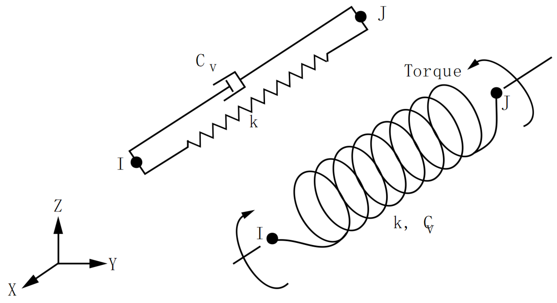
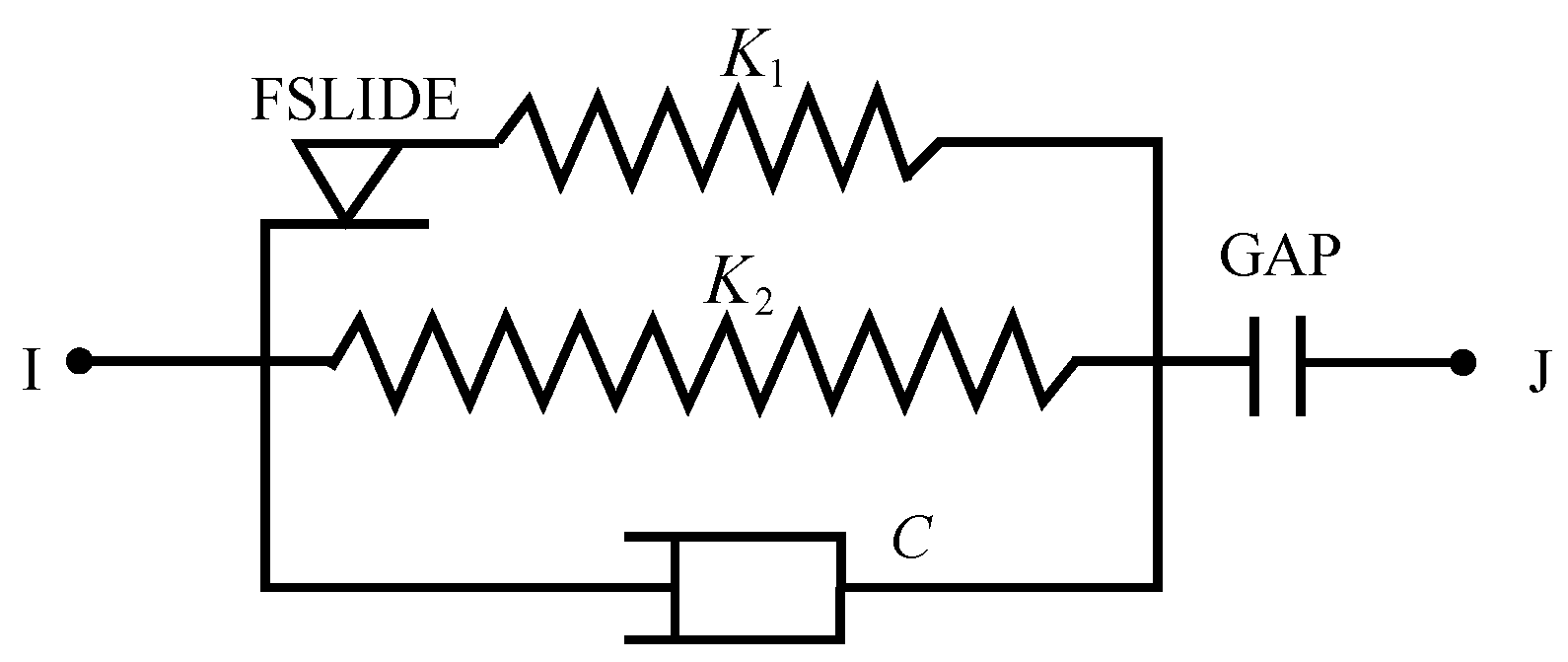
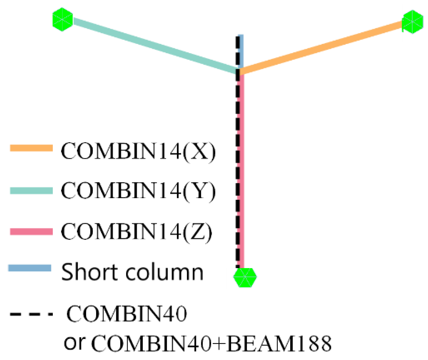
22] analyzed the elastic connection element of MIDAS and the COMBIN14 element of ANSYS. And found that for the axial expansion torsion problem, the two are similar to the stiffness matrix of ordinary beam element, which can be simulated by COMBIN14 element. However, only one-dimensional stiffness can be set. In ANSYS, three COMBIN14 elements are used for the simulation. Without considering the element damping, the schematic diagram of the COMBIN14 element is shown in
Figure 9 [
23,
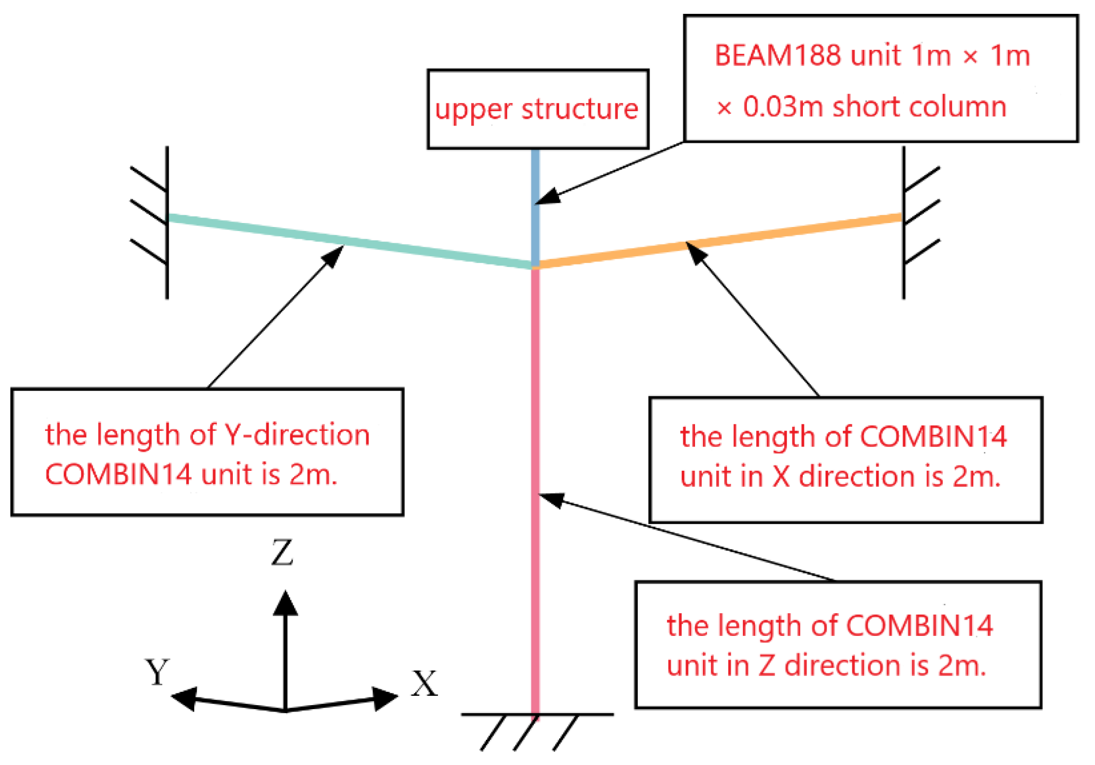
24]. The original spring connection node is stretched downward into a short column of 1.0m × 1.0m × 0.03m. The short column is short, while its cross section and the stiffness are large. It can be considered as a rigid rod. Three COMBIN14 elements are arranged along the X, Y and Z directions. The element length is 2m and the stiffness is distributed axially, as shown in
Figure 10.
However, the elastic connection unit plays different roles in different models. In this theater model, the elastic connection unit simulates the spring. And it is possible to connect the components. If the elastic connection is used for the connection between the components, the two nodes can be connected by coupling degrees of freedom. Different conversion methods can be set according to different needs.
(6) Anti-rocking structure simulation
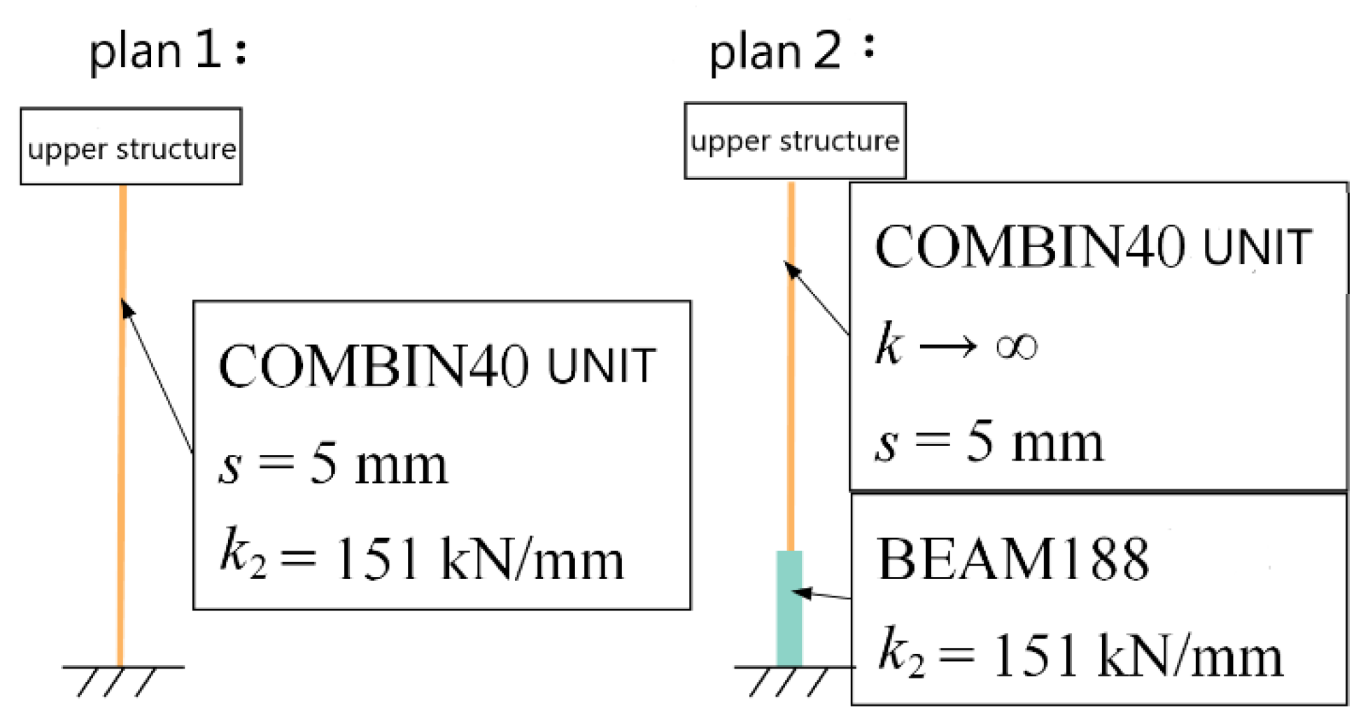
The mechanical properties of the anti-rocking structure are special. The stiffness and yield strength of the steel tie rod need to be adjusted, considering the initial play of the steel tie rod. Two simulation schemes of the anti-rocking structure are proposed, as shown in
Figure 11. Scheme 1 is simulated by a single COMBIN40 element and scheme 2 is simulated by COMBIN40 + BEAM188 plastic beam element in series.
The element properties of COMBIN40 are shown in
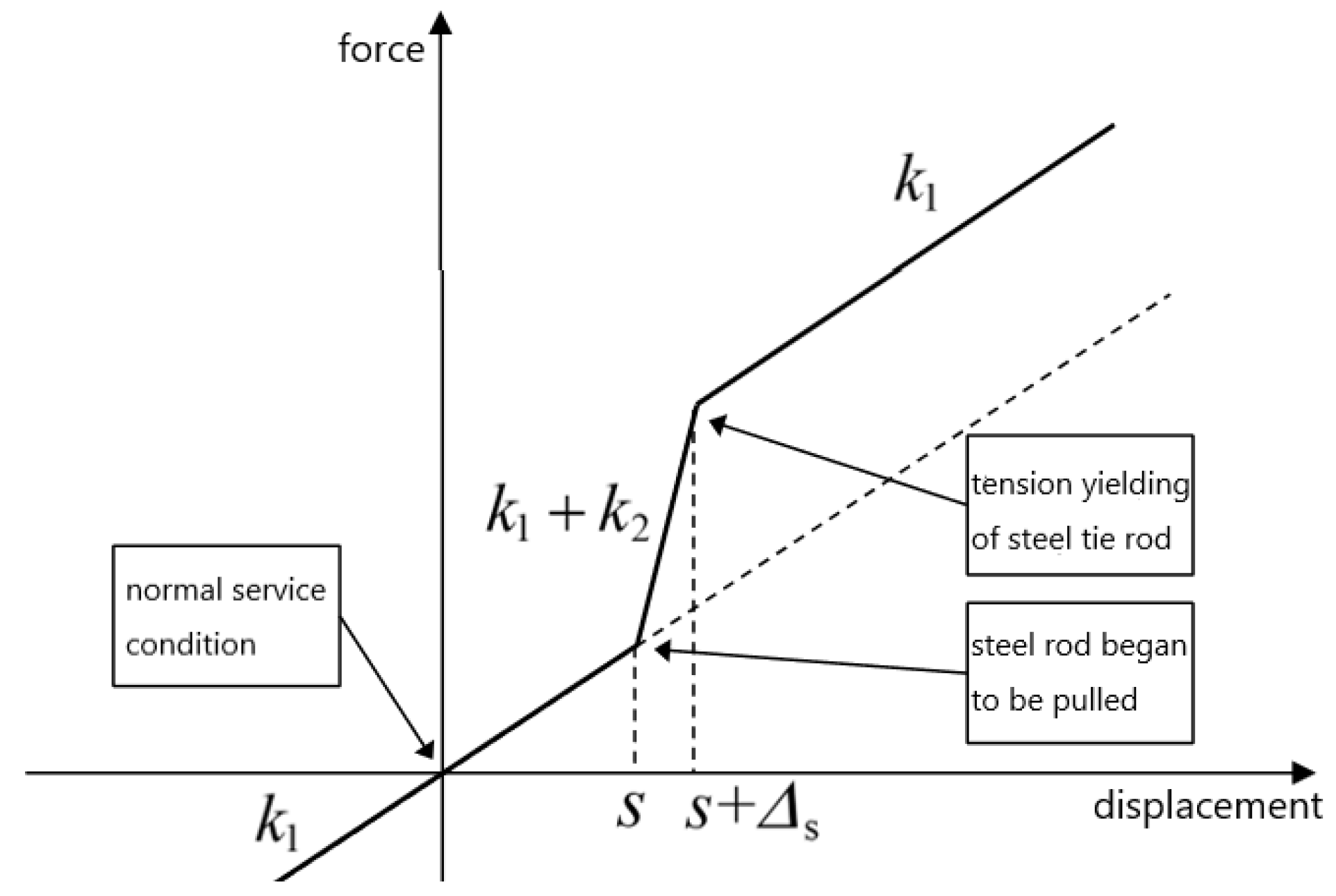
Figure 12 [
23]. The element includes initial gap, element stiffness (k1) and (k2), element slip force and element damping(C). The element stiffness can be used to simulate the stiffness of the steel tie rod. The element slip force can be used to approximate the yield force of the steel tie rod and the element initial gap can be used to simulate the initial gap of the steel tie rod. COMBIN40 whose stiffness is set to a maximum value only considers the initial clearance of the steel tie rod. It is considered to be a rigid rod and the element stiffness is provided by the BEAM188 element. Using the bilinear element and the Von Mises yield criterion, the element yield can be considered.
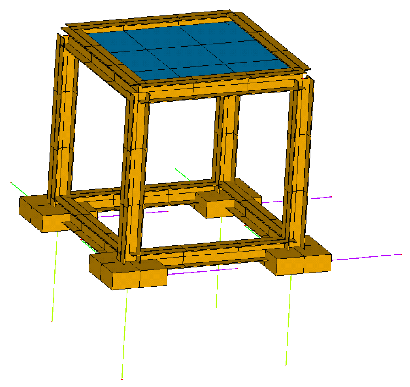
To analyze the difference between the actual analysis results of the two schemes, a three-dimensional frame model is established in ANSYS, as shown in
Figure 13 and
Figure 14. The anti-rocking structure is arranged according to the two schemes and the dynamic time history analysis is carried out. The ground motion time history wave adopts the Taft wave and the acceleration is loaded in three directions.
Figure 15 illustrates the vertical displacement curves of the bearings in the two layout schemes. As illustrated in the diagram, upon the initial application of the seismic wave, the three-way displacement curves of the No. 4 bearing unit in the two scheme models exhibit a high degree of coincidence. As the steel rod is subjected to continuous tensile strain, the peak displacement of the two is observed to differ. However, the discrepancy is not significant. The maximum discrepancy in displacement in the X and Y directions is 1.0% and 1.8%, respectively. The maximum discrepancy in the Z-direction displacement is 7.25%. A comparison of the three-dimensional displacement curves of X, Y and Z reveals that as the seismic wave loading time is extended continuously, the degree of coincidence between the displacement curves of the two schemes increases once more. Ultimately, the displacement curves converge. This may be attributed to the failure of the steel tie rod in the anti-rocking structure, which may have been caused by excessive stretching. Following the failure of the steel tie rod, the anti-rocking device will cease to function, resulting in a gradual alignment of the displacement curve. Furthermore, the values of X, Y and Z three-way displacements in the non-overlapping section of the curve in Scheme 1 are higher than those in Scheme 2. This indicates that the limiting effect of the anti-rocking device on the vertical displacement of the bearing and the anti-rocking effect of the device are underestimated when only the COMBIN40 element is used.
Nevertheless, when compared with the analysis results of Scheme 1 and Scheme 2, it can be observed that the difference between the node displacement and the anti-rocking effect is not significant. Furthermore, Scheme 2 is capable of more realistically and accurately simulating the anti-rocking device. However, both the COMBIN40 spring element and the BEAM188 plastic beam element in the second scheme are nonlinear elements, which makes achieving convergence in the calculation process a significant challenge. At the same time, the calculation time for the two groups of models is markedly disparate. Under the two groups of schemes, the finite element calculation time for the small model in
Figure 13 is approximately 10 minutes and 2 hours, respectively. Therefore, the difference is considerable. The first scheme can greatly reduce the software calculation time.
In summary, it is more feasible and effective to use the first scheme to simulate the anti-rocking device. The Python conversion program encompasses the necessary programs for both schemes, which can be selected based on the specific requirements.

