Preprint
Article

Carbon-Neutral Forestry Contributes to Global Warming due to Carbon Debt

Altmetrics

Downloads

56

Views

52

Comments

0

A peer-reviewed article of this preprint also exists.

This version is not peer-reviewed

Submitted:

04 October 2024

Posted:

07 October 2024

You are already at the latest version

Alerts
Abstract
This article presents an evaluation of the environmental impact of forestry based on landscape theory. It has been argued that this type of forestry offers a positive impact on the climate because there is a balance between the amount of greenhouse gas emissions and the absorption of these gases within an entire forested area. However, this analysis will demonstrate that the arrangement and composition of managed forests are linked to a significant carbon debt. This debt represents the disparity between the carbon that would typically be stored in a natural forest and the actual amount of carbon stored in the managed forest. While this excess carbon remains in the atmosphere rather than being sequestered, it contributes to the greenhouse effect. Using the Swedish forestry as an example, the carbon debt is estimated to be comparable in scale to the total accumulated fossil fuel emissions of the country.
Keywords: 
Subject: Environmental and Earth Sciences  -   Environmental Science

1. Introduction

The climate impact resulting from forestry is influenced by various factors, including rotation time (the period between final fellings), harvest volume (the amount of timber extracted), and the lifespan of wood products. There is still no scientific consensus regarding whether harvesting woody biomass for energy or other purposes provides any climate benefits, considering the specific timeframes outlined in climate targets. The primary concern revolves around the time required for the harvested forest to regrow, which is commonly referred to as the "payback time." This period plays a crucial role in determining whether the carbon emissions associated with biomass harvesting can be offset by subsequent regrowth and carbon sequestration [1,2,3,4]. According to a study on Finnish forestry [5], it was found that the payback time, which includes the recovery of soil, is estimated to be between 90 and 110 years. However, another study demonstrated that repeated logging can lead to a reduction in soil organic carbon over several centuries [6]. Additionally, ref. [7] concludes that substantial carbon sequestration continues for at least 50 to 100 years beyond the typical economic rotation periods (which range from 80 to 120 years in boreal forests). Indeed, it has been observed that the conclusions drawn in many studies regarding forestry optimized for climate benefits are influenced by the methodological assumptions employed. For instance, certain studies suggest that increased harvest would yield climate mitigation benefits rely on assumptions such as enhanced carbon storage after harvest through fertilization or an expansion of forested areas. Those are very uncertain propositions [8,9]
The concept of substitution effects is another important aspect to consider. In theory, forestry can offer a relative climate benefit if biomass is used as a substitute for products that currently rely on fossil fuels, including construction materials like concrete. However, substitution theory is implicitly based on the assumptions that there are no viable alternatives to replace fossil fuels and that the products or processes in question are unavoidable. Nonetheless, numerous efforts have been made to quantify the potential substitution effects and evaluate their impact on climate mitigation. As an example, studies such as [10] have shown that replacing fossil fuels with corn ethanol could potentially result in a slight climate benefit. However, in the case of woody biomass, the potential for substitution effects can be counterproductive [9,11].
When crops are grown for energy purposes on agricultural land, the time between plantings is typically brief, often lasting only one year. However, if the agricultural land was previously covered by forests that were cleared to make way for the crops, a carbon debt is incurred due to the loss of the forest biomass. When accounting for this carbon debt, it has been discovered that the actual climate impact of using crops as fuel can be as significant as that of certain fossil fuels [12] and even worse than fossils [13]. Also, it has been suggested that substitution benefits have been overestimated by 2-100 times [14]. A recent study concludes that when leaving biofuel emission untaxed, as it is today, the climate impact could be just as high as for fossil fuels [15].
Pay-back times for boreal forests of the order of 100 years are much too long to address political climate targets [7]. However, boreal forestry is typically managed across vast areas, which allows for the creation of a landscape structure corresponding to a mosaic of same aged tree stands with an even age distribution among the stands. By logging not more than the yearly growth, the net carbon flow to the atmosphere will be close to zero and the forestry becomes “carbon-neutral” [16]. However, in the IPCC scenarios the role of managed forests in mitigating the climate crisis is to provide a substantial net uptake of carbon [17]. Therefore, ‘bioenergy must be evaluated by addressing both the stocks and flows of the carbon cycle’, as was pointed out in [18]. In the recent IPCC report AR6, an increased uptake of carbon through restoring and protecting forests as well as improved forest management are pointed out as a climate mitigation strategy with high potential [19]. As a side note, restoration of forests is necessary for the purpose of saving biodiversity as well as re-paying the carbon debt [20]. For a comprehensive summary, see [21].
Although estimate of carbon debt are somewhat approximate, since it depends on uncertain reference levels, it has been clarified that the potential uptake is an adequate measure of carbon debt [22]. The potential of carbon sequestration was estimated for Swedish [23] and Finnish [24] forest land and found to be substantial in both cases.
The concept of a "carbon debt" is frequently misconstrued as being solely tied to the payback times of managed land. This misconception can lead to the conclusion that shorter payback times result in negligible carbon debt. As a result, left-over products with shorter decomposition times are often claimed to have short payback times, leading to the assumption that these products are inherently climate beneficial when used as fuel [25,26]. Such conclusions will be questioned in this paper.
The main objective of this paper is to examine the carbon debt linked to landscape theory. The theoretical landscape forestry model, as presented by the International Energy Agency (IEA) Bioenergy working group [27], has mistakenly conflated the terms "carbon-neutral" and "climate-neutral." From a policymaking perspective, it is indeed crucial to distinguish between these two concepts.

2. Methods

2.1. Qualitative Overview

The IEA landscape theory is based on two relevant concepts that need to be defined. Firstly, it is necessary to provide a definition of the notion of a landscape [28]. There are multiple interpretations of this concept in the existing literature. In accordance with the Kyoto Protocol on land-use change and forestry (LULUCF), the appropriate understanding of a landscape encompasses an entire nation, including both managed and non-managed forests. [29]. However, considering the climate impact of forestry itself, using the entire nation as the landscape can result in misleading results. Therefore, the EU green taxonomy [30] adopts a different approach, defining the relevant landscape as that of a single company or forest owner. These entities are required to regularly provide a climate benefit protocol to assess their specific impact on the climate.
The second undefined parameter in the IEA landscape theory is the period for assessing the climate impact. For the sake of convenience, the IEA has chosen a period of one year. This choice aligns with the time frame of the climate crisis and is compatible with standard national accounting systems.
If the landscape is organized into a theoretical grid, comprising the same number of units as the rotation time for forestry in years, it is possible to achieve precise compensation of logged biomass through growth, provided each stock unit within the grid has a distinct and unique age. For instance, if the rotation time is set at 100 years, one can envision structuring the landscape as a grid consisting of 100 units. The stands within this grid would then have ages ranging from 0 to 100 years, with the oldest stand subject to logging. By following this approach, the total amount of biomass remains constant within a given year, ensuring that no carbon is released into the atmosphere.
The landscape structure can naturally emerge when working with a sufficiently large area, such as a nation with abundant forests. By selectively logging only mature stands, a landscape structure gradually takes shape over time.
Most forests are managed in this way and today’s forests in Europe are overall a carbon sink [31,32], i.e. the carbon uptake is greater than the forestry emission as defined in LULUCF. If forestry is carbon-neutral and the total national forest provides a carbon sink, it is tempting to argue that European forestry is climate beneficial [33], and it is easy to convey this argument to politicians. Is such a conclusion accurate?
In what follows, it will be demonstrated that the landscape theory is incomplete. It overlooks the initial conditions involved in shaping the landscape structure. That is, it neglects the carbon that was stored in natural and mature forests before large-scale forestry commenced.

2.2. Analytical Approach

To assess the landscape theory in a simple, yet quantitative manner, we start by examining a hypothetical forestry scenario with a four-year rotation time. Subsequently, we extend this analysis to include a forestry system with an arbitrary rotation time. The general formula for the carbon debt is attained using method of induction. To establish a direct connection with the results of the IEA, our analysis is founded on the same theoretical framework as the IEA's. The forestry is depicted in an idealized manner, consisting of only single-species trees, and in this scenario, all the trees within a single grid are logged. The logged trees are instantly converted to CO2, and new trees begin to grow immediately. While this representation may not be entirely realistic, it adopts basic and simplistic forestry principles, making it a fundamental framework for analysis. Indeed, a more realistic representation of forestry can be achieved by incorporating corrections to this model. As our results are mathematically formulated, it is feasible to include these corrections, allowing for a more accurate depiction of real-world forestry conditions.

3. Results

3.1. General

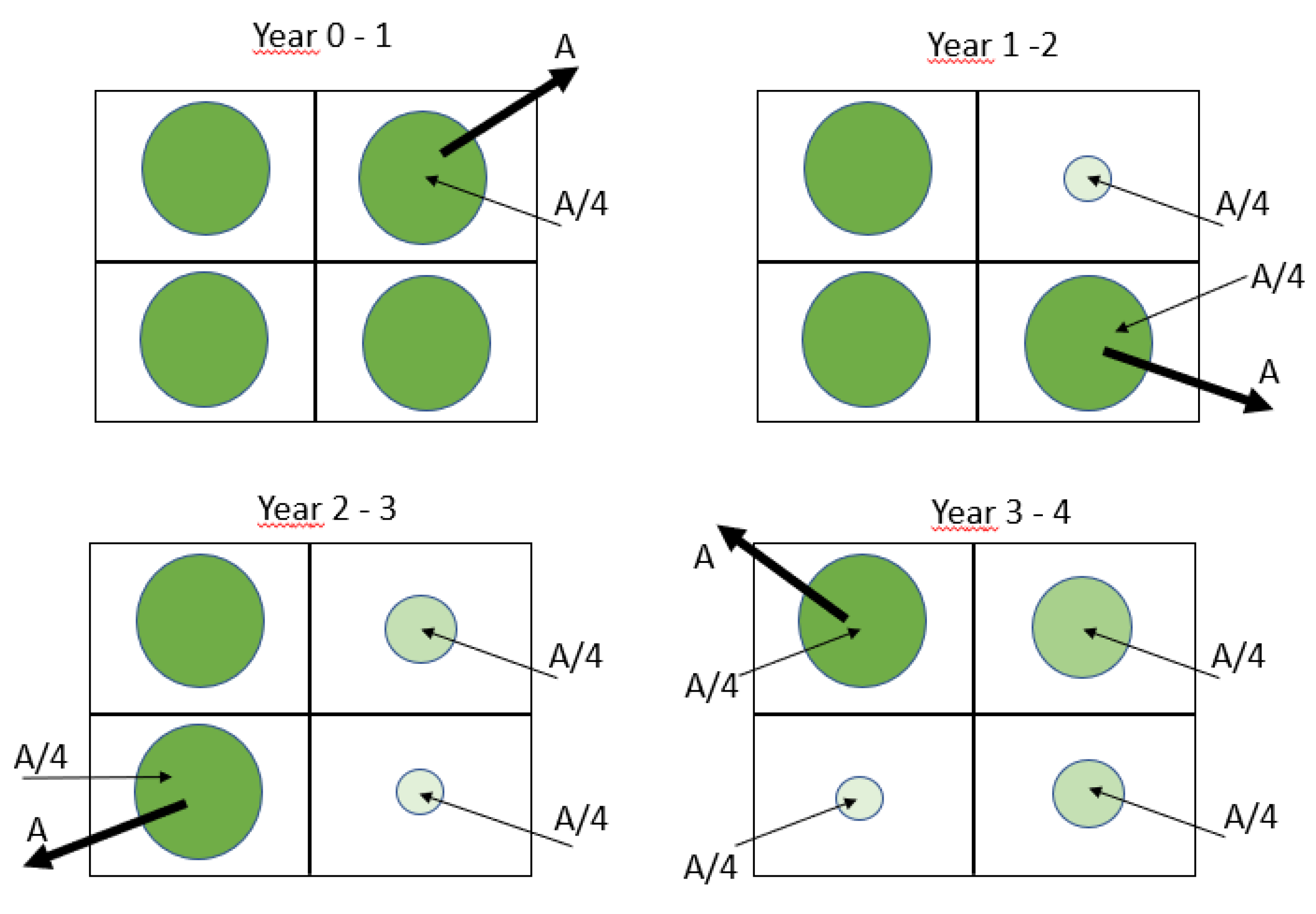
The IEA landscape theory is depicted in Figure 1, specifically illustrating a forestry system with a four-year rotation time.
The landscape comprises a grid consisting of four units. The unit with a mature stand is logged. The growth for one year will compensate for the emission A at combustion, assuming all logging converts to CO2. Next year, another grid is logged and the procedure repeats. This approach claims to achieve a forestry system that is sustainable and climate-neutral.
However, for a comprehensive analysis, it is necessary to consider the initial conditions. It can be presumed that a natural forest was initially present in the forestry area. In order to establish a forestry system with a structured landscape, one grid unit is clear-cut each year, as depicted in Figure 2.
After four years, the landscape structure has been established. However, the total biomass present in the landscape is now smaller compared to the original natural forest. By accounting for the carbon outflux (due to harvest) and carbon influx (from growth) and comparing it to the initial carbon storage of the natural forest, there is a carbon deficit equivalent to 6/16 of the original natural forest. This number is obtained by comparing the final amount of biomass to that of the original forest. Initially there is an amount of 4A in biomass. In the final state there is A + 3/4A + 2/4A + 1/4A = 10/4A. The deficit becomes 4A – 10/4A = 6/4A. Dividing by the initial content we get 6/16 in fractional deficit.
This deficit is never fully compensated for or paid back within the forestry system. In addition, this carbon debt is likely an underestimate because natural forests typically contain more biomass compared to mature forestry plantations. Natural forests possess older trees, higher biodiversity, a greater abundance of dead wood, and intact underground vegetation [6,34,35,36].
Consider now a more realistic forestry with rotation time of one hundred years, typical for a boreal forest composed of conifers. The calculation below is under the assumption that after one rotation period the forest has regrown completely. Thus, it assumes that the rotation period equals the regrowth time. In reality, the regrowth time may be much longer [7].
The grid consists of 100 units and after 100 years of logging one unit per year, the landscape structure is established. Each unit has then a unique stand age which is evenly distributed from 1-100 years within the landscape. For example, the grid unit with stand age 100 years was logged 100 years ago and has recovered all its original biomass. The 50 years old grid unit was logged 50 years ago and consists of half its original biomass whereas the youngest grid was logged the last year and has recovered no biomass.
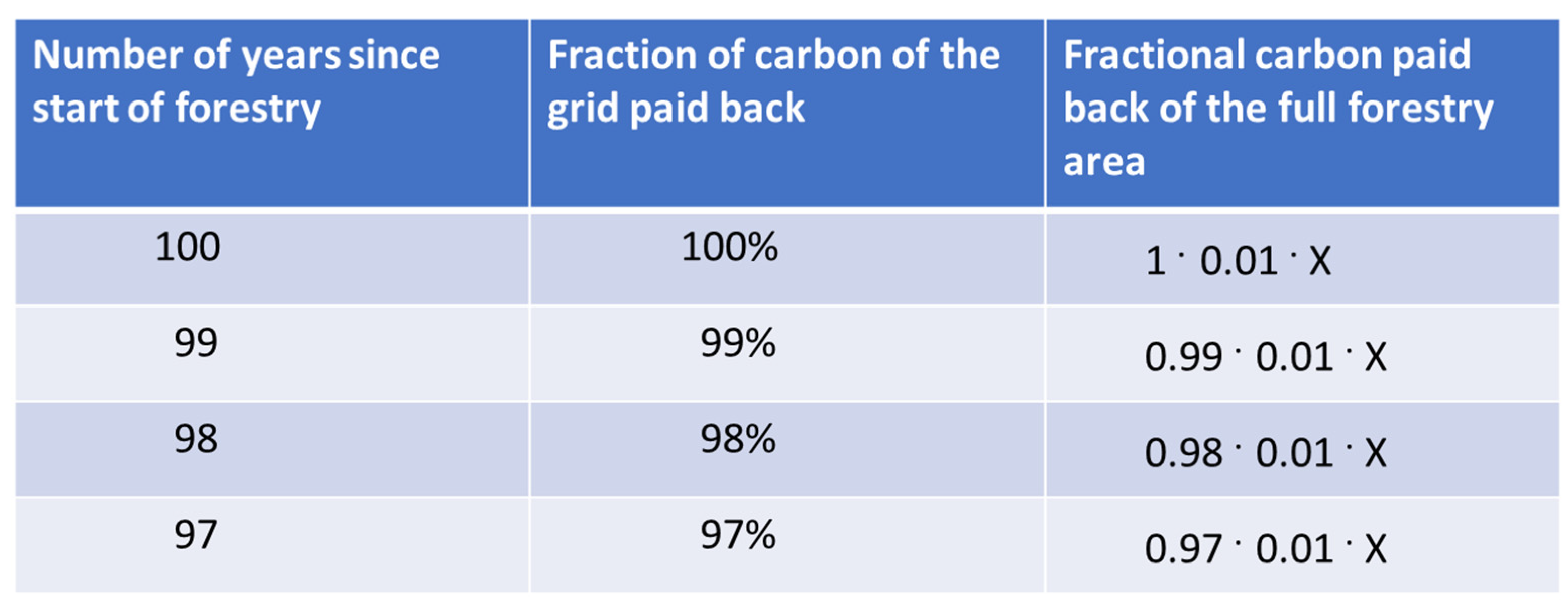
Table 1 Paid back carbon for the four oldest grid units in a 100-years forestry 100 years after start of logging. Each grid unit comprises 1% of the total forestry area which is reflected in the factor 0.01 in the third column. X is the total amount of original biomass.
Only the first logged grid unit is fully compensated. Following the logic of Table 1, the carbon debt D becomes:
D = n = 1 100 1 n ε 0.01 X = X 0.01 X ε n = 1 100 n = 0.5 X
where ε = 0.01 for an evenly distributed growth per year. In reality ε = ε(n), i.e. it varies with the stand age so that the assumed constant value should be considered as an average. Thus, the carbon debt corresponds to half the biomass of the original natural forest.
In general, the carbon dept for a landscape structured forestry with rotation time N years becomes
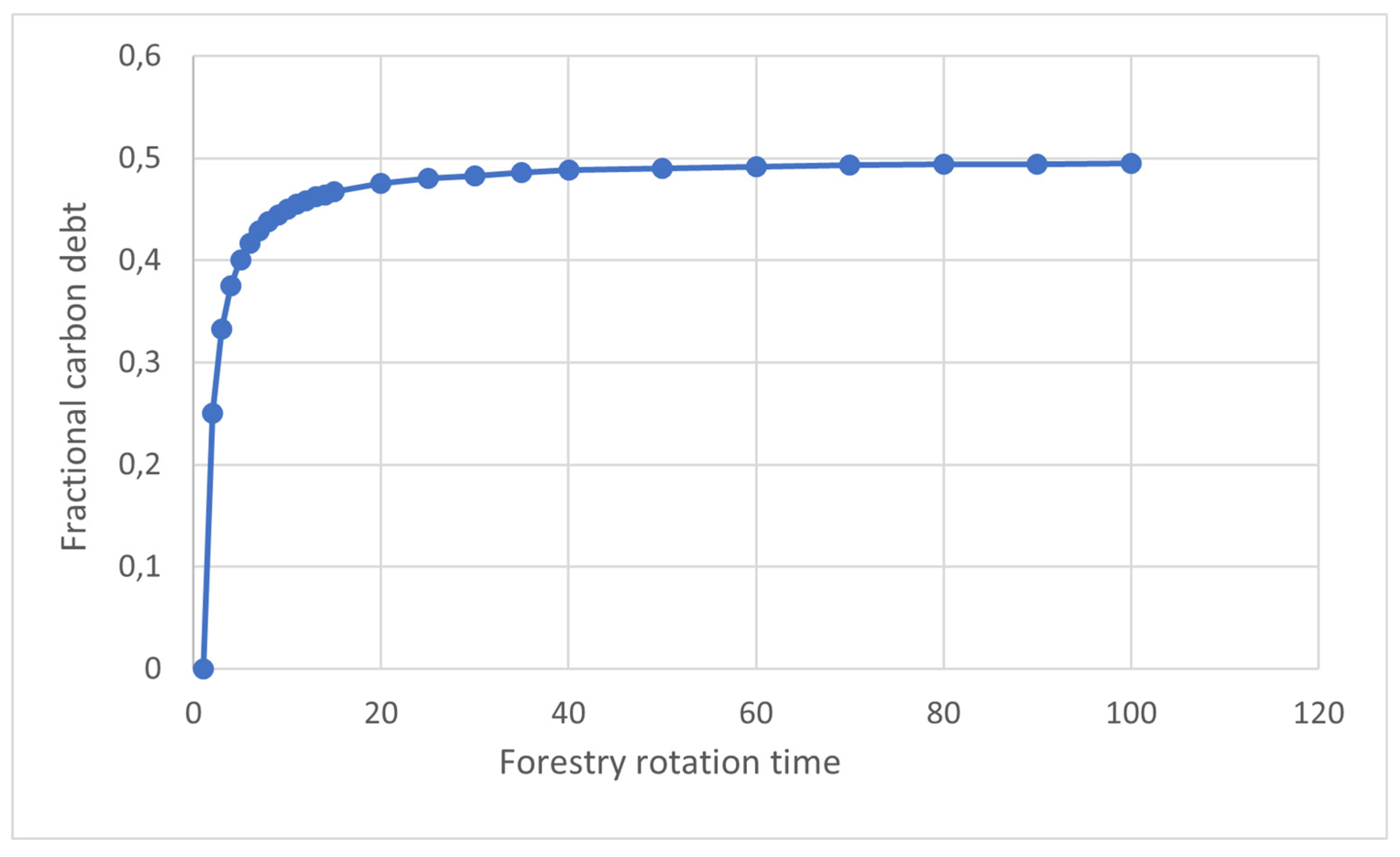
D ( N ) = X X N 2 n = 1 N n X X N 2 N 2 N = 1 2 X
where the approximation is valid for large rotations time N in years.
Formula (2) is plotted in Figure 3 demonstrating the limiting value of a 50% carbon dept.
The conclusion of this analysis is that a typical forestry incurs a carbon debt equal to at least the same amount as the carbon content of the managed forest. As a result of the biomass deficit, there is a notable contribution to the excess carbon in the atmosphere. Consequently, the forestry system cannot be regarded as climate-neutral because the "missing" carbon directly contributes to global warming.
To estimate the carbon debt for a real forestry it is convenient to consider a full nation, utilizing official statistics. In this regard, an analysis will be presented based on Sweden, which is one of the world's most forestry-intensive countries.

3.2. Case Study: Sweden

Sweden's forest cover amounts to 70%, of which 70% is actively managed. The forestry practice in Sweden utilizes almost exclusively the technique based on clearing, thinning, clear-cutting, land scarification, and single-species replantation. The supply of bioenergy in Sweden is abundant, and it currently serves as the largest source of combustion energy, providing approximately half of the country's heat energy [37].
The forestry rotation time in Sweden is notably long, with approximately 80 years for southern spruce plantations and 120 years for northern pine plantations. As a result, the annual clear-cut area represents approximately 1% of the total managed area of 20 MHa. Each year, approximately 90 Mm3 of stem volume is harvested from the forests [38]. Half of this amount is due to thinning taking place twice during a rotation time.
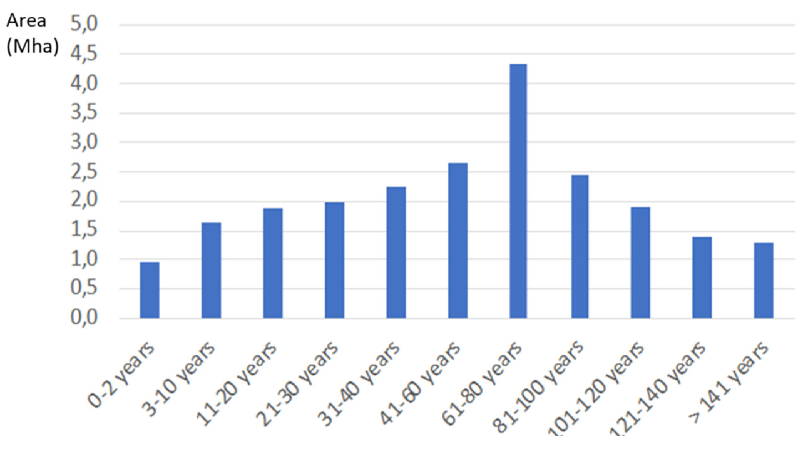
The landscape grid structure of the forestry has evolved successively while being managed. Starting from a landscape consisting partly of natural forest and partly of non-sustainable forestry land, together with abandoned agricultural and pastureland about 100 years ago, the landscape slowly transformed to something close to a landscape structure, Figure 4 [39]. However, the landscape is not a regular grid, as discussed in the previous section, but the units are spread out in the country as a mosaic.
According to Swedish statistics the forestry carbon stock (living biomass above ground) is estimated to be 3000 Mm3 stem volume. Based on our estimation, this would correspond to at most half the biomass volume originally stored in natural forests and therefore represent the minimum carbon debt.
According to UN guidelines, 1.0 m3 stem volume has absorbed 1.4 tons of carbon dioxide [40]. This factor takes into account the full tree, i.e. including branches, tops, roots and stumps. Sweden’s carbon debt therefore can be estimated to be at least 4200 Mton CO2, close to the nation’s accumulated fossil emissions of 5000 Mton [41].
This estimated carbon debt is in line with predictions [23] made using the Heureka software package [42] to model the growth of the Swedish forest given different logging intensities. If logging were to cease altogether, the Heureka calculations estimated an initial average uptake of 1.4 tonnes carbon per hectare and year, which would increase somewhat first and slow down eventually, depending on region. The aggregate carbon sequestration predicted by these calculations for a completely unmanaged forest would be approximately 10 000 Mton CO2 over 100 years which is about twice the value we gave for the carbon debt. This is reasonable since our estimate is based on a non-changed climate and a forestry rotation time equal to the regrowth time, forming a lower limit of the potential uptake. However, in reality the growth will continue well beyond the forestry rotation time and due to CO2 fertilization the growth will be enhanced [43,44].

3.2.1. Swedish Total Climate Gas Emissions

According to official statistics, emissions from Swedish forestry amount to 120 Mton CO2 annually. This number is a five-year average centered on year 2018 [40]. If forestry activities were to cease completely, the emissions from the forestry sector would no longer occur. Instead, these emissions would contribute to the carbon sink as the forest would have the opportunity to maximize its carbon uptake. Initially, the forest would experience a high rate of carbon absorption, which would gradually decrease over time as the forest reaches a mature stage. This gradual decrease in carbon uptake would ultimately lead to a balance where the carbon absorption equals the carbon release through natural processes in the ecosystem. During the time it takes for a forest to go from the end of logging activities to becoming a mature forest, the average amount of carbon absorbed by the forest would be roughly half of the maximum amount it can absorb, i.e. 60 Mton. Therefore, over a rotation time of 80-120 years the carbon debt would be paid back, as expected [23].
When evaluating the country's overall climate impact, it is therefore reasonable to consider the contribution from forestry based on its emissions. Hence, when considering the country's annual fossil emissions of 50 million tons of CO2, an additional 120 Mton “missed carbon sequestration” due to forestry should be included. This results in a total emission of 170 Mton, which corresponds to 17 tons per inhabitant per year. This method of evaluating the climate impact from forestry is endorsed by a recent study [43]. How does this compare to the total emissions of other countries?
IEA has released an analysis of energy supply sources for various nations [37]. While the fossil emissions for each country are well documented and studied [41], estimating biogenic emissions has proven to be challenging until now. The available data provides information on the total energy supplied by biogenic sources in different countries. However, the actual biogenic emissions are influenced by specific forestry practices, including factors like rotation time, harvested volume, and the proportion of long-lived products. Hence, only an estimation of biogenic emissions can be made under the assumption of consistent forestry and forest industry practices. In this scenario, the emissions are considered to be proportionate to the utilization of bioenergy.
Based on Figure 5 in the IEA report [37], an approximate comparison can be made between Sweden and the USA, with the latter often being referred to as one of the highest greenhouse gas emitters per capita worldwide. However, per capita bioenergy usage in the USA is only one-sixth of that in Sweden, obtaining a result as in Table 2.
Thus, Sweden can be considered as one of the global leaders in terms of greenhouse gas emissions. While Sweden's forestry practices may be considered "carbon neutral" in terms of net emissions, the substantial carbon debt associated with its forestry operations significantly contributes to the climate crisis. As a result, it cannot be regarded as "climate-neutral". This viewpoint is consistent with the IPCC pathways and the EU's climate law, which emphasize the importance of increasing carbon uptake in addressing climate change. For instance, already in 2030 Sweden is required to increase its forest carbon sink from the current 10 Mton [44] to 54 Mton. This entails significant demands for reduced logging.
Note that the LULUCF regulation is incomplete in this respect. While it correctly reports the annual net emission from the land sector, it fails to clarify the historical carbon debt. This shortcoming may be resolved by reporting emissions and uptake separately, rather than just their difference.

4. Discussion

In this paper, we analyzed the carbon debt due to forestry, with Sweden as a case study. In the analysis we assumed that all forestry products are instantaneously converted to carbon dioxide. While this is an approximation, it closely reflects reality. In Sweden, less than 10% of the logging is processed into long-lived lumber. More than half of the harvested biomass is directly combusted, including the use of black liquor in the paper and pulp industries, and around 30% of the harvest becomes short-lived paper products [45]. The latter becomes waste after a few years and is used as fuel in central heating plants. Even lumber has a finite lifetime with an estimated half-time of around 35 years. Therefore, within the typical rotation time of forestry operations, almost all products, including lumber, have been converted to carbon dioxide. This justifies the approximation made in the analysis.
We have also left out a detailed analysis of the difference between a plantation and natural forest. For example, the carbon content below ground and effects from forest fires influences the analysis. Whereas the former could only work to the detriment of the plantation, the occurrence of forest fires is less frequent in managed forests [33]. However, it has been found that forest fires leave more than 90% of the biomass in the forest intact as dead wood [46,47,48,49], indicating that a forest fire does not have a large impact on the carbon stock. Nevertheless, [33] parallels a forest fire with a clear cut, claiming clear-cutting mimics natural processes. Obviously, this claim has no support.
The carbon content of the soil, comprising around 50% of the total carbon content of a boreal forest, is not discussed in detail here. In brief, the dynamics of the soil has a significant impact on the emissions from forestry and it has been shown that repeated harvest leads to a permanent reduction in the amount of soil carbon [6]. For Swedish forestry it has been estimated that 10-20% of the total emissions originate from decomposition of dead organic material left after a clear-cut felling [50]. Loss of soil carbon therefore contributes to the carbon debt.
The validity of the concept of a carbon debt for carbon-neutral forestry has been questioned since the amount of living biomass above ground in Swedish forests has continuously increased over the past century [33]. However, it is important to note that when modern forestry practices were initiated, not all forested areas were natural forests. Some portions of the land included abandoned agricultural land, pastureland, and unsustainable forestry practices. The replanting efforts in these areas have indeed led to a significant increase in the amount of living biomass above ground in the forests. However, this observation does not alter our conclusion regarding carbon debt. This is because if we look further back in time, these lands were originally covered by natural forests that possessed a considerably larger carbon stock [51]. Alternatively, the potential of uptake can be considered [22]. This potential has been assessed through computer simulations, yielding results consistent with our analysis [23]. Moreover, it has been demonstrated that the growing carbon stock in forests worldwide is connected to the surplus of carbon in the atmosphere caused by human activities and their emissions [52].
In addition to the climate crisis, there is a biodiversity crisis [53] that is interconnected with forestry. The decline in biodiversity also has adverse consequences for the climate, as mono-cultural forests have been found to contain significantly lower levels of stored biomass [34]. To define forestry methods that do not meet sustainability standards, EU regulation makes use of concepts such as ‘deforestation’ and ‘forest degradation’. The term 'forest degradation' refers to forestry practices that pose a threat to ecosystems and biodiversity [54]. Examples of such practices include clear-cutting, scarification, and monocultural replanting, which are observed in the forestry practices of countries like Sweden and Finland. In this light, forestry is far from sustainable in these countries [55,56]

5. Conclusions

The landscape theory of forestry proposed by the IEA was investigated and shown to be incomplete. It fails to consider the initial stage of landscape forestry formation. Consequently, it overlooks the carbon debt that arises during this stage, as the forestry is only potentially half filled with biomass. An estimation of the carbon debt for Sweden indicates that the biogenic contribution to atmospheric carbon is comparable in magnitude to the accumulated fossil contribution. When accounting for biogenic emissions, it was found that Sweden is among the world leaders in terms of emission per capita. This finding contradicts official statements made by Sweden claiming to be world leaders in climate mitigation.
In accordance with IPCC, the atmospheric surplus of CO2 has two main sources: emissions from fossil fuels and loss of biomass. Restoring and protecting forests and increasing carbon uptake are equally important as reducing fossil fuel emissions. Consequently, almost all proposals to substitute fossil energy sources with biomass should be seen as counterproductive.

Data Availability Statement

All data used is included in the article.

Conflicts of Interest

The authors confirm no conflict of interests.

References

  1. J. R. Malcolm, B. Holtsmark, and P. W. Piascik. Forest harvesting and the carbon debt in boreal east-central Canada. Clim Change 2020, 161, 433–449. [Google Scholar] [CrossRef]
  2. S. R. Mitchell, M. E. Harmon, and K. E. B. O’Connell. Carbon debt and carbon sequestration parity in forest bioenergy production. GCB Bioenergy 2012, 4, 818–827. [Google Scholar] [CrossRef]
  3. E. -D. Schulze, C. Körner, B. E. Law, H. Haberl, and S. Luyssaert. Large-scale bioenergy from additional harvest of forest biomass is neither sustainable nor greenhouse gas neutral. GCB Bioenergy 2012, 4, 611–616. [Google Scholar] [CrossRef]
  4. G. Zanchi, N. Pena, and N. Bird. Is woody bioenergy carbon neutral? A comparative assessment of emissions from consumption of woody bioenergy and fossil fuel. GCB Bioenergy 2012, 4, 761–772. [Google Scholar] [CrossRef]
  5. Repo, J.-P. Tuovinen, and J. Liski. Can we produce carbon and climate neutral forest bioenergy? GCB Bioenergy 2015, 7, 253–262. [Google Scholar] [CrossRef]
  6. Dean, J. B. Kirkpatrick, and A. J. Friedland. Conventional intensive logging promotes loss of organic carbon from the mineral soil. Glob Chang Biol 2017, 23, 1–11. [Google Scholar] [CrossRef] [PubMed]
  7. J. N. Stokland. Volume increment and carbon dynamics in boreal forest when extending the rotation length towards biologically old stands. For Ecol Manage 2021, 488, 119017. [Google Scholar] [CrossRef]
  8. N. S. Bentsen. Carbon debt and payback time – Lost in the forest? Renewable and Sustainable Energy Reviews 2017, 73, 1211–1217. [Google Scholar] [CrossRef]
  9. S. Soimakallio, T. Kalliokoski, A. Lehtonen, and O. Salminen. On the trade-offs and synergies between forest carbon sequestration and substitution. Mitig Adapt Strateg Glob Chang 2021, 26, 4. [Google Scholar] [CrossRef]
  10. M. Q. Wang, J. Han, Z. Haq, W. E. Tyner, M. Wu, and A. Elgowainy. Energy and greenhouse gas emission effects of corn and cellulosic ethanol with technology improvements and land use changes. Biomass Bioenergy 2011, 35, 1885–1896. [Google Scholar] [CrossRef]
  11. P. Leturcq. GHG displacement factors of harvested wood products: the myth of substitution. Sci Rep 2020, 10, 20752. [Google Scholar] [CrossRef] [PubMed]
  12. V. Daioglou et al. Greenhouse gas emission curves for advanced biofuel supply chains. Nat Clim Chang 2017, 7, 920–924. [Google Scholar] [CrossRef]
  13. T. D. Searchinger, S. Wirsenius, T. Beringer, and P. Dumas. Assessing the efficiency of changes in land use for mitigating climate change. Nature 2018, 564, 249–253. [Google Scholar] [CrossRef]
  14. M. E. Harmon. Have product substitution carbon benefits been overestimated? A sensitivity analysis of key assumptions. Environmental Research Letters 2019, 14, 065008. [Google Scholar] [CrossRef]
  15. L. Merfort et al. Bioenergy-induced land-use-change emissions with sectorally fragmented policies. Nat Clim Chang, 2023. [CrossRef]
  16. H. Haberl et al. Correcting a fundamental error in greenhouse gas accounting related to bioenergy. Energy Policy 2012, 45, 18–23. [Google Scholar] [CrossRef]
  17. M. Babiker et al. Cross-sectoral perspectives. In IPCC, 2022: Climate Change 2022: Mitigation of Climate Change. Contribution of Working Group III to the Sixth Assessment Report of the Intergovernmental Panel on Climate Change. 2022. [CrossRef]
  18. J. M. DeCicco and W. H. Schlesinger. Reconsidering bioenergy given the urgency of climate protection. Proceedings of the National Academy of Sciences 2018, 115, 9642–9645. [Google Scholar] [CrossRef]
  19. P. R. et al. Shukla. Climate Change 2022: Mitigation of Climate Change. Working Group III Contribution to the IPCC Sixth Assessment Report. 2022. [CrossRef]
  20. S. L. Lewis, C. E. Wheeler, E. T. A. Mitchard, and A. Koch. Restoring natural forests is the best way to remove atmospheric carbon. Nature 2019, 568, 25–28. [Google Scholar] [CrossRef] [PubMed]
  21. M. Rogers et al. Using ecosystem integrity to maximize climate mitigation and minimize risk in international forest policy. Frontiers in Forests and Global Change 2022, 5. [Google Scholar] [CrossRef]
  22. K. -H. Erb et al. Unexpectedly large impact of forest management and grazing on global vegetation biomass. Nature 2018, 553, 73–76. [Google Scholar] [CrossRef]
  23. T. Skytt, G. Englund, and B.-G. Jonsson. Climate mitigation forestry—temporal trade-offs. Environmental Research Letters 2021, 16, 114037. [Google Scholar] [CrossRef]
  24. J. Seppälä et al. Effect of increased wood harvesting and utilization on required greenhouse gas displacement factors of wood-based products and fuels. J Environ Manage 2019, 247, 580–587. [Google Scholar] [CrossRef] [PubMed]
  25. T. Hammar and F. Levihn. Time-dependent climate impact of biomass use in a fourth generation district heating system, including BECCS. Biomass Bioenergy 2020, 138, 105606. [Google Scholar] [CrossRef]
  26. Thiffault, A. Gianvenuti, X. Zuzhang, and S. Walter, The role of wood residues in the transition to sustainable bioenergy. FAO, 2023. [CrossRef]
  27. L. Cowie et al. Applying a science-based systems perspective to dispel misconceptions about climate effects of forest bioenergy. GCB Bioenergy 2021, 13, 1210–1231. [Google Scholar] [CrossRef]
  28. Deahl, L. Walloe, and M. Norton. EASAC Open Letter to IEA-Bioenergy.” Accessed: Feb. 11, 2023. [Online]. Available: https://easac.eu/news/details/iea-bioenergy-critique-of-easac-publications-on-forest-bioenergy/.
  29. United Nations Climate Change. Reporting and accounting of LULUCF activities under the Kyoto Protocol. 2008. Accessed: Feb. 19, 2023. [Online]. Available: https://unfccc.int/topics/land-use/workstreams/lulucf-under-the-kyoto-protocol/reporting-and-accounting-of-lulucf-activities-under-the-kyoto-protocol.
  30. European Commission. Taxonomy Regulation. https://ec.europa.eu/finance/docs/level-2-measures/taxonomy-regulation-delegated-act-2021-2800-annex-1_en.pdf.
  31. S. Luyssaert et al. The European carbon balance. Part 3: forests. Glob Chang Biol 2010, 16, 1429–1450. [Google Scholar] [CrossRef]
  32. Le, Quéré; et al. Global Carbon Budget 2018. Earth Syst Sci Data 2018, 10, 2141–2194. [Google Scholar] [CrossRef]
  33. P. Högberg et al. Sustainable boreal forest management – challenges and opportunities for climate change mitigation. 2021, Accessed: Feb. 20, 2023. [Online]. Available: https://www.skogsstyrelsen.se/globalassets/om-oss/rapporter/rapporter-20222021202020192018/rapport-2021-11-sustainable-boreal-forest-management-challenges-and-opportunities-for-climate-change-mitigation-002.pdf.
  34. Y. Huang et al. Impacts of species richness on productivity in a large-scale subtropical forest experiment. Science (1979) 2018, 362, 80–83. [Google Scholar] [CrossRef]
  35. Merino, C. Real, J. G. Álvarez-González, and M. A. Rodríguez-Guitián. Forest structure and C stocks in natural Fagus sylvatica forest in southern Europe: The effects of past management. For Ecol Manage 2007, 250, 206–214. [Google Scholar] [CrossRef]
  36. H. Keith, B. G. Mackey, and D. B. Lindenmayer. Re-evaluation of forest biomass carbon stocks and lessons from the world’s most carbon-dense forests. Proceedings of the National Academy of Sciences 2009, 106, 11635–11640. [Google Scholar] [CrossRef]
  37. L. Pelkman. IEA Bioenergy Countries’ Report – update 2021. IEA Bioenergy https://www.ieabioenergy.com/wp-content/uploads/2021/11/CountriesReport2021_final.pdf.
  38. Swedish Forest Agency. Forestry Production. https://www.skogsstyrelsen.se/en/statistics/.
  39. S. Swedish Official Statistics. Skogsdata 2022. Umeå, 2022. Accessed: May 13, 2023. [Online]. Available: https://www.slu.se/globalassets/ew/org/centrb/rt/dokument/skogsdata/skogsdata_2022_webb.pdf.
  40. Swedish Environmental Protection Agency. UN GHG National Inventiry Report Sweden.” Accessed: Feb. 11, 2023. [Online]. Available: https://unfccc.int/documents/461776.
  41. M. Crippa, D. Guizzardi, E. Solazzo, and M. Muntean. European Commission, JRC Report: GHG emissions of all world countries. 2021. Accessed: Feb. 11, 2023. [Online]. Available: https://data.europa.eu/doi/10.2760/173513.
  42. P. Wikström et al. THE HEUREKA FORESTRY DECISION SUPPORT SYSTEM: AN OVERVIEW. Mathematical and Computational Forestry & Natural-Resource Sciences 2011, 3, 87–94. [Google Scholar]
  43. L. Peng, T. D. L. Peng, T. D. Searchinger, J. Zionts, and R. Waite. The carbon costs of global wood harvests. Nature, 2023. [Google Scholar] [CrossRef]
  44. S. U. Department of Forest Resource Management. Skogsdata (Forest data) 2023. https://www.slu.se/globalassets/ew/org/centrb/rt/dokument/skogsdata/skogsdata_2023_webb.pdf.
  45. IRENA. Bioenergy from boreal forests: Swedish approach to sustainable wood use. Abu Dhabi, 2019. Accessed: Feb. 25, 2023. [Online]. Available: https://www.irena.org/-/media/Files/IRENA/Agency/Publication/2019/Mar/IRENA_Swedish_forest_bioenergy_2019.pdf.
  46. H. Keith et al. Accounting for Biomass Carbon Stock Change Due to Wildfire in Temperate Forest Landscapes in Australia. PLoS One 2014, 9, e107126. [Google Scholar] [CrossRef]
  47. M. E. Harmon, C. T. Hanson, and D. A. DellaSala. Combustion of Aboveground Wood from Live Trees in Megafires, CA, USA. Forests 2022, 13, 391. [Google Scholar] [CrossRef]
  48. G. W. Meigs, D. C. Donato, J. L. Campbell, J. G. Martin, and B. E. Law. Forest Fire Impacts on Carbon Uptake, Storage, and Emission: The Role of Burn Severity in the Eastern Cascades, Oregon. Ecosystems 2009, 12, 1246–1267. [Google Scholar] [CrossRef]
  49. J. Campbell, D. Donato, D. Azuma, and B. Law. Pyrogenic carbon emission from a large wildfire in Oregon, United States. J Geophys Res Biogeosci 2007, 112, G4. [Google Scholar] [CrossRef]
  50. Lindroth. Clarifying the carbon balance recovery time after clear-cutting. Glob Chang Biol 2023, 29, 4178–4179. [Google Scholar] [CrossRef] [PubMed]
  51. P. Linder and L. Östlund. Structural changes in three mid-boreal Swedish forest landscapes, 1885–1996. Biol Conserv 1998, 85, 9–19. [Google Scholar] [CrossRef]
  52. C. Davis, B. Sohngen, and D. J. Lewis. The effect of carbon fertilization on naturally regenerated and planted US forests. Nat Commun 2022, 13, 5490. [Google Scholar] [CrossRef]
  53. Dinerstein, *!!! REPLACE !!!*; et al. A Global Deal For Nature: Guiding principles, milestones, and targets. Sci Adv 2019, 5. [Google Scholar] [CrossRef]
  54. European Parlament. Deforestation Regulation. https://www.europarl.europa.eu/doceo/document/TA-9-2022-0311_EN.pdf.
  55. K. B. Lindahl et al. The Swedish forestry model: More of everything? For Policy Econ 2017, 77, 44–55. [Google Scholar] [CrossRef]
  56. P. Angelstam et al. Sweden does not meet agreed national and international forest biodiversity targets: A call for adaptive landscape planning. Landsc Urban Plan 2020, 202, 103838. [Google Scholar] [CrossRef]
Figure 1. Schematic of a landscape forestry which for illustrative reasons is assumed to have a rotation time of four years. The quantity A indicates the carbon loss due to harvest and A/4 is the average influx of carbon due to sequestration in one grid unit annually. In this manner, the CO2 uptake equals the loss. Note though, that this is a simplified approach since in reality the uptake is not linear with time in each individual stand. However, the average rate of growth over a large enough landscape in a steady state is constant by definition.
Preprints 120261 g001
Figure 2. The carbon flow during the initial formation of a landscape forestry. Only about half the carbon is stored in the final landscape forestry compared to the initial state.
Preprints 120261 g002
Figure 3. Fractional carbon debt vs. forestry rotation time in years. The carbon debt is close to 50% of the original carbon content of the forest.
Preprints 120261 g003
Figure 4. Areal distribution of forest ages in Sweden. There is an approximate even distribution of same age stands. Note that the age intervals are not equal.
Preprints 120261 g004
Table 1. shows the amount of paid back carbon for each grid unit in the last few years, with X representing total initial biomass.
Preprints 120261 i001
Table 2. Approximate emission per capita (Mton CO2 per year) for Sweden and the USA.
Fossil Biogenic Total
Sweden 5 12 17
USA 16 2 18
Disclaimer/Publisher’s Note: The statements, opinions and data contained in all publications are solely those of the individual author(s) and contributor(s) and not of MDPI and/or the editor(s). MDPI and/or the editor(s) disclaim responsibility for any injury to people or property resulting from any ideas, methods, instructions or products referred to in the content.
Copyright: This open access article is published under a Creative Commons CC BY 4.0 license, which permit the free download, distribution, and reuse, provided that the author and preprint are cited in any reuse.
Prerpints.org logo

Preprints.org is a free preprint server supported by MDPI in Basel, Switzerland.

Subscribe

© 2024 MDPI (Basel, Switzerland) unless otherwise stated