
Submitted:
05 October 2024
Posted:
07 October 2024
Read the latest preprint version here
Abstract
The importance of continuously emerging new distribution is a mandate to understand the world and environment surrounding us. In this paper, the author will discuss a new distribution defined on the interval (0,1) as regards the methodology of deducing its PDF, some of its properties and related functions. A simulation and real data analysis will be highlighted.
Keywords:
Median based unit Rayleigh (MBUR) distribution
; new distribution
; unit distribution
; Maximum product of spacing
; MLE
Introduction
Fitting data to a statistical distribution helps to understand the phenomenon of the data generating process behind them. Researchers have developed many different distributions to describe complex real world phenomena. Before 1980, the techniques used to generate distributions were mainly: solving systems of differential equations, using transformations and lastly using quantile function strategy. After 1980, the procedures used are mainly summarized into either adding new parameters to an existing distribution or combining all-ready known distributions. These maneuvers provide researchers with a wide spectrum of tractable and flexible distributions that can accommodate all variety of asymmetrical data as well as outliers in the data sets. Fitting distributions to data helps to better model the data in analyses involving regression, survival analysis, reliability analysis and time series analysis.
Many authors used regression models like location-scale regression to model Egyptian stock exchange as proposed by Salah Mahdy and Samy Abdelmoez (Abdelmoezz & Mohamed, 2021) and to model survival time in myeloma patients by Mahmoud Riad et al. (2015).
Also Quantile regression models are used by many authors to model time to event response variables which exhibit skewness with long tails as well as violation of normality and homogeneity assumptions. These models are robust to outlier, skewness, and heteroscedasticity as they specify the entire conditional distribution of the response variable rather than the conditional mean. Many authors applied this type of regression to measure the effects of covariates on the time duration response variable at different quantiles. To mention some of them: Flemming et al. studied association between time to surgery and survival among patients suffering from cancer colon (Flemming et al., 2017). Faradmal et al. applied censored quantile regression to examine overall factors affecting survival in breast cancer (Faradmal et al., 2016). Xue et al. thoroughly explored the censored quantile regression model to analyze time to event data (Xue et al., 2018).
Many real world phenomena are presented as proportions, ratios, or fractions over the bounded unit interval (0,1). Modelling these data in different disciplines like biology, finance, mortality rate, recovery rate, economics, engineering, hydrology, health, and measurement sciences had been achieved by many authors using continuous distributions.
Some of these distributions are:
Johnson SB distribution (Johnson, 1949).
Beta distribution (Eugene et al., 2002).
- (1)
- Unit Johnson (SU ) distribution (Gündüz & Korkmaz, 2020).
- (2)
- Topp- Leone distribution (Topp & Leone, 1955).
- (3)
- Unit Gamma (Consul & Jain, 1971; Grassia, 1977; Mazucheli et al., 2018; Tadikamalla, 1981).
- (4)
- Unit Logistic distribution (Tadikamalla & Johnson, 1982).
- (5)
- Kumaraswamy distribution (Kumaraswamy, 1980).
- (6)
- Unit Burr-III (Modi & Gill, 2020).
- (7)
- Unit modified Burr-III (Haq et al., 2023).
- (8)
- Unit Burr-XII (Korkmaz & Chesneau, 2021).
- (9)
- Unit-Gompertz (Mazucheli, Maringa, et al., 2019).
- (10)
- Unit-Lindely (Mazucheli, Menezes, et al., 2019).
- (11)
- Unit-Weibull (Mazucheli et al., 2020).
- (12)
- Unit Muth distribution (Maya et al., 2024).
Unit distribution is mostly obtained by variable transformation. The transformation can take any form of the followings: , , or The paper is arranged into 4 sections. In section 1, the author will explain the methodology of obtaining the new distribution. In section 2, elaboration of its PDF,CDF, Survival function, Hazard function and reversed hazard function will be presented. In section 3, methods of estimation will be discussed accompanied by simulation study. In section 4, real data analysis will be achieved with discussion.
Section 1
Methodology:
Derivation of the MBUR Distribution:
Using the pdf of median order statistics for sample size=3 and parent distribution Rayleigh :
Using the following transformation:
So the new distribution is the Median Based Unit Rayleigh (MBUR) Distribution.
Section 2
Some of the properties of the new distribution ( MBUR):
- The following is the pdf :
- 2.
- The following is the CDF:
- 3.
- The following is the survival function :
- 4
- The following is the hazard function (hf) and reversed hazard function (rhf) respectively:
The following figures, Figure 1, Figure 2, Figure 3, Figure 4, Figure 5, Figure 6, Figure 7, Figure 8 and Figure 9, show the above functions for different values of alpha:
1. Quantile Function:
The inverse of the CDF is used to obtain y , the real root of this 3rd polynomial function is :
To generate random variable distributed as MBUR:
- 1-
- Generate uniform random variable (0,1):
- 2-
- Choose alpha.
- 3-
- Substitute the above values of u (0,1) and the chosen alpha in the quantile function, to obtain y distributed as
- 2-
- rth Raw Moments:
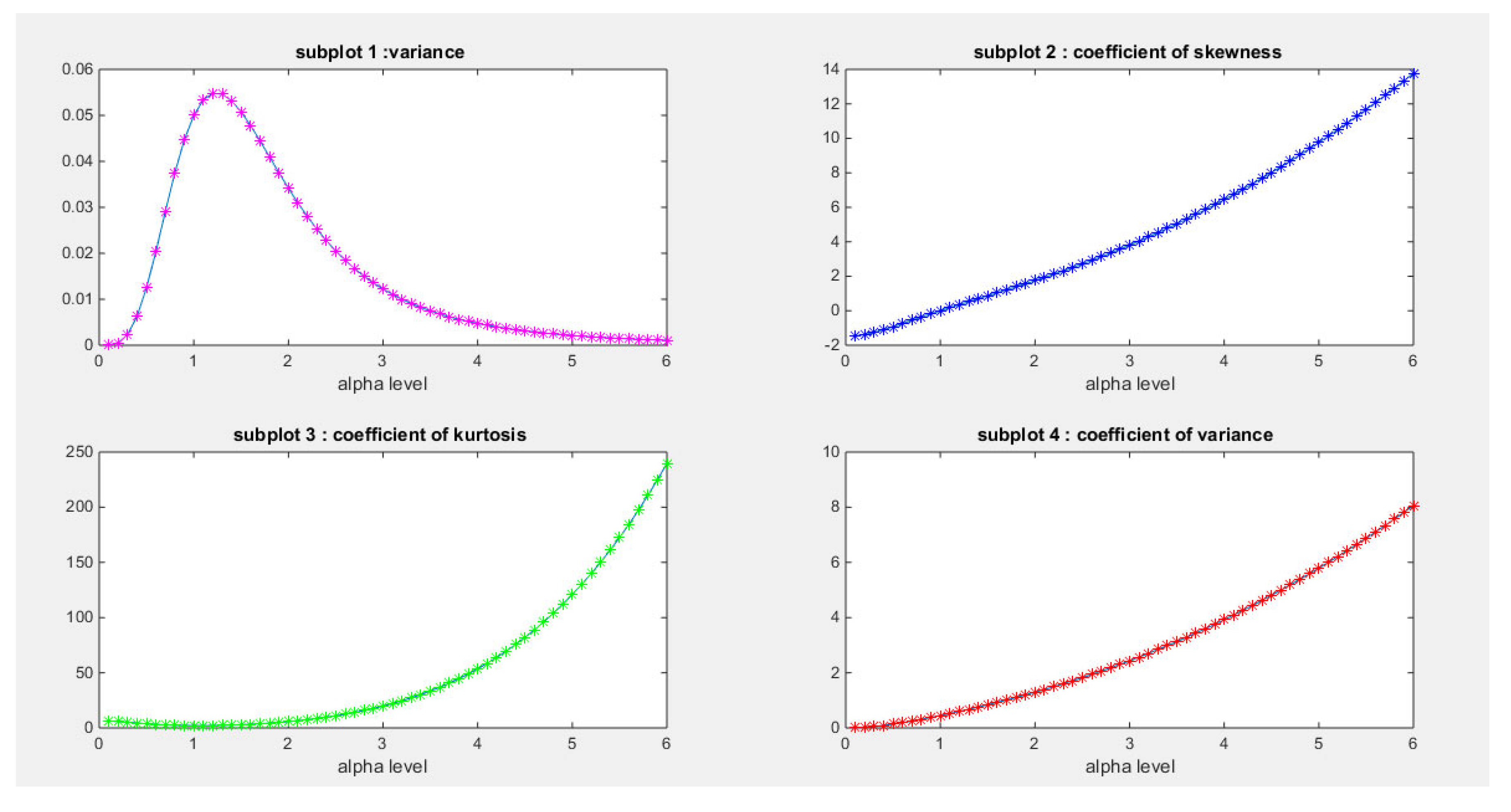
3. Coefficient of Skewness:
4. Coefficient of Kurtosis:
5. Coefficient of Variation :
The following Figure 10 illustrate the graph for above coefficients
- 6.
- rth incomplete Moments:
Section 3:
Methods of Estimations:
- Method of Moments:
Equating the first moment from the sample which is the mean with that from the population can be used to estimate the parameter. Then this estimate can be used as initial guess in other methods that need numerical techniques to evaluate the parameter.
To find the estimator for the alpha parameter, find the root of the following equation:
- 2.
- Maximum Likelihood Estimation :
Alpha can be estimated numerically using Newton Raphson method.
3. Maximum Product of Spacing ( MPS) :
Maximize the following objective function:
Alpha can be estimated numerically using Newton Raphson method.
- 4.
- Anderson Darling Estimator (AD)
Minimize the following objective function:
Alpha can be estimated numerically using Newton Raphson method.
- 5.
- Percentile method :
Minimize the following objective function:
Alpha can be estimated numerically using Newton Raphson method.
- 6.
- Cramer Von Mises(CVM)
Minimize the following objective function:
Alpha can be estimated numerically using Newton Raphson method.
- 7.
- Least Squares Method:
Minimize the following objective function:
Alpha can be estimated numerically using Newton Raphson method.
- 8.
- Weighted Least Squares Method:
Alpha can be estimated numerically using Newton Raphson method.
Section 3:
Simulation
A simulation study is conducted using the following sample sizes , and replicate N=1000 times. The different kinds of methods of estimation are utilized and compared with each other. The alpha values chosen are .
Steps:
- Generate random variable from the MBUR Distribution with specified alpha
- Chose the sample size n.
- Replicate the method of estimation N times .
-
Calculate the following metrics to compare between the methods and show the effect of increasing sample size on the estimators.
- (a)
- (b)
- (c)
- (d)
Also the mean of estimated alpha from the 1000 replicate is evaluated with the standard error.
For the chosen alpha level (2.5), the following results are obtained in the successive tables, mean(1), SE(2), AAB(3), MSE(4), MRE(5):

Table 1.
mean.
| mean | MOM | MLE | MPS | AD | PERC | CVM | LS | WLS |
| n=20 | 2.6 | 2.4911 | 2.5321 | 2.5067 | 2.3617 | 2.4697 | 2.5274 | 2.5327 |
| n=80 | 2.52 | 2.486 | 2.5043 | 2.4896 | 2.4445 | 2.4896 | 2.4908 | 2.4943 |
| n=160 | 2.5069 | 2.4936 | 2.5039 | 2.495 | 2.4524 | 2.4953 | 2.496 | 2.4977 |
| n=260 | 2.5030 | 2.4972 | 2.5042 | 2.4991 | 2.4782 | 2.5004 | 2.5008 | 2.5008 |
Table 2.
Table 2. SE.
| SE | MOM | MLE | MPS | AD | PERC | CVM | LS | WLS |
| n=20 | 0.013 | 0.0065 | 0.0065 | 0.0067 | 0.0123 | 0.0088 | 0.0078 | 0.0071 |
| n=80 | 0.0057 | 0.0033 | 0.0032 | 0.0034 | 0.0065 | 0.0037 | 0.0037 | 0.0035 |
| n=160 | 0.0041 | 0.0022 | 0.0022 | 0.0024 | 0.0045 | 0.0025 | 0.0025 | 0.0024 |
| n=260 | 0.0031 | 0.0018 | 0.0018 | 0.0019 | 0.0039 | 0.0012 | 0.0012 | 0.0019 |
Table 3.
AAB.
| AAB | MOM | MLE | MPS | AD | PERC | CVM | LS | WLS |
| n=20 | 0.3221 | 0.1592 | 0.1631 | 0.1663 | 0.3296 | 0.194 | 0.1916 | 0.1785 |
| n=80 | 0.1444 | 0.0827 | 0.0809 | 0.085 | 0.1754 | 0.0902 | 0.0901 | 0.0854 |
| n=160 | 0.1037 | 0.0561 | 0.0552 | 0.0595 | 0.1127 | 0.0626 | 0.0625 | 0.0596 |
| n=260 | 0.0791 | 0.0457 | 0.0456 | 0.0481 | 0.0995 | 0.0506 | 0.506 | 0.0481 |
Table 4.
MSE.
| MSE | MOM | MLE | MPS | AD | PERC | CVM | LS | WLS |
| n=20 | 0.1798 | 0.0418 | 0.0427 | 0.045 | 0.1701 | 0.0791 | 0.0617 | 0.0516 |
| n=80 | 0.0333 | 0.0119 | 0.0102 | 0.012 | 0.0451 | 0.0137 | 0.0137 | 0.0120 |
| n=160 | 0.0166 | 0.0051 | 0.0048 | 0.0057 | 0.0226 | 0.0063 | 0.0063 | 0.0056 |
| n=260 | 0.0098 | 0.0032 | 0.0032 | 0.0036 | 0.0153 | 0.004 | 0.004 | 0.0036 |
Table 5.
MRE.
| MRE | MOM | MLE | MPS | AD | PERC | CVM | LS | WLS |
| n=20 | 0.1288 | 0.0637 | 0.0652 | 0.0665 | 0.1318 | 0.2813 | 0.0766 | 0.0714 |
| n=80 | 0.0578 | 0.0331 | 0.0324 | 0.0340 | 0.0702 | 0.0361 | 0.0361 | 0.0342 |
| n=160 | 0.0415 | 0.0224 | 0.0221 | 0.0238 | 0.0451 | 0.025 | 0.025 | 0.0238 |
| n=260 | 0.0317 | 0.0183 | 0.0182 | 0.0192 | 0.0398 | 0.0202 | 0.0202 | 0.0192 |
The author is working on the n=500 and on the other values of alpha.
As shown from the tables increasing sample size decreases the SE, AAB, MSE and MRE. The methods show comparable results as regards the estimation value no big difference is there among them.
Section 4:
Some Real Data Analysis:
The data sets are obtained from the site of OECD which stands for Organization for Economic Co-operation and Development, it provides data about the economy, social events, education, health, labor, and environment in the countries involved in the organization. The data is available at https://stats.oecd.org/index.aspx?DataSetCode=BLI
First data: (Dwelling Without Basic Facilities)
These observations measure the percentage of homes in the involved countries that lack essential utilities like indoor plumbing, central heating, clean drinking water supplies.
| 0.008 | 0.007 | 0.002 | 0.094 | 0.123 | 0.023 | 0.005 | 0.005 | 0.057 | 0.004 |
| 0.005 | 0.001 | 0.004 | 0.035 | 0.002 | 0.006 | 0.064 | 0.025 | 0.112 | 0.118 |
| 0.001 | 0.259 | 0.001 | 0.023 | 0.009 | 0.015 | 0.002 | 0.003 | 0.049 | 0.005 |
| 0.001 |
Second data : (Quality of Support Network)
This data set explores how much the person can rely on sources of support like family, friends, or community members in time of need and disparate. It is represented as percentage of persons who had found social support in times of crises.
| 0.98 | 0.96 | 0.95 | 0.94 | 0.93 | 0.8 | 0.82 | 0.85 | 0.88 | 0.89 |
| 0.78 | 0.92 | 0.92 | 0.9 | 0.96 | 0.96 | 0.94 | 0.77 | 0.95 | 0.91 |
Third data : ( Educational Attainment )
The oservations measure the percentage of population in the OECD database that completed their high level of education like high school or equivalent.
| 0.84 | 0.86 | 0.8 | 0.92 | 0.67 | 0.59 | 0.43 | 0.94 | 0.82 | 0.91 |
| 0.91 | 0.81 | 0.86 | 0.76 | 0.86 | 0.76 | 0.85 | 0.88 | 0.63 | 0.89 |
| 0.89 | 0.94 | 0.74 | 0.42 | 0.81 | 0.81 | 0.93 | 0.55 | 0.92 | 0.9 |
| 0.63 | 0.84 | 0.89 | 0.42 | 0.82 | 0.92 |
Fourth data : ( Flood Data)
These are 20 observations for the maximum flood level in Susquehanna River at Harrisburg, Penssylvania (Dumonceaux & Antle, 1973) .
| 0.26 | 0.27 | 0.3 | 0.32 | 0.32 | 0.34 | 0.38 | 0.38 | 0.39 | 0.4 |
| 0.41 | 0.42 | 0.42 | 0.42 | 045 | 0.48 | 0.49 | 0.61 | 0.65 | 0.74 |
Fifth data : ( Time between Failures of Secondary Reactor Pumps)(Maya et al., 2024, 1999)(Suprawhardana and Prayoto)
| 0.216 | 0.015 | 0.4082 | 0.0746 | 0.0358 | 0.0199 | 0.0402 | 0.0101 | 0.0605 |
| 0.0954 | 0.1359 | 0.0273 | 0.0491 | 0.3465 | 0.007 | 0.656 | 0.106 | 0.0062 |
| 0.4992 | 0.0614 | 0.532 | 0.0347 | 0.1921 |
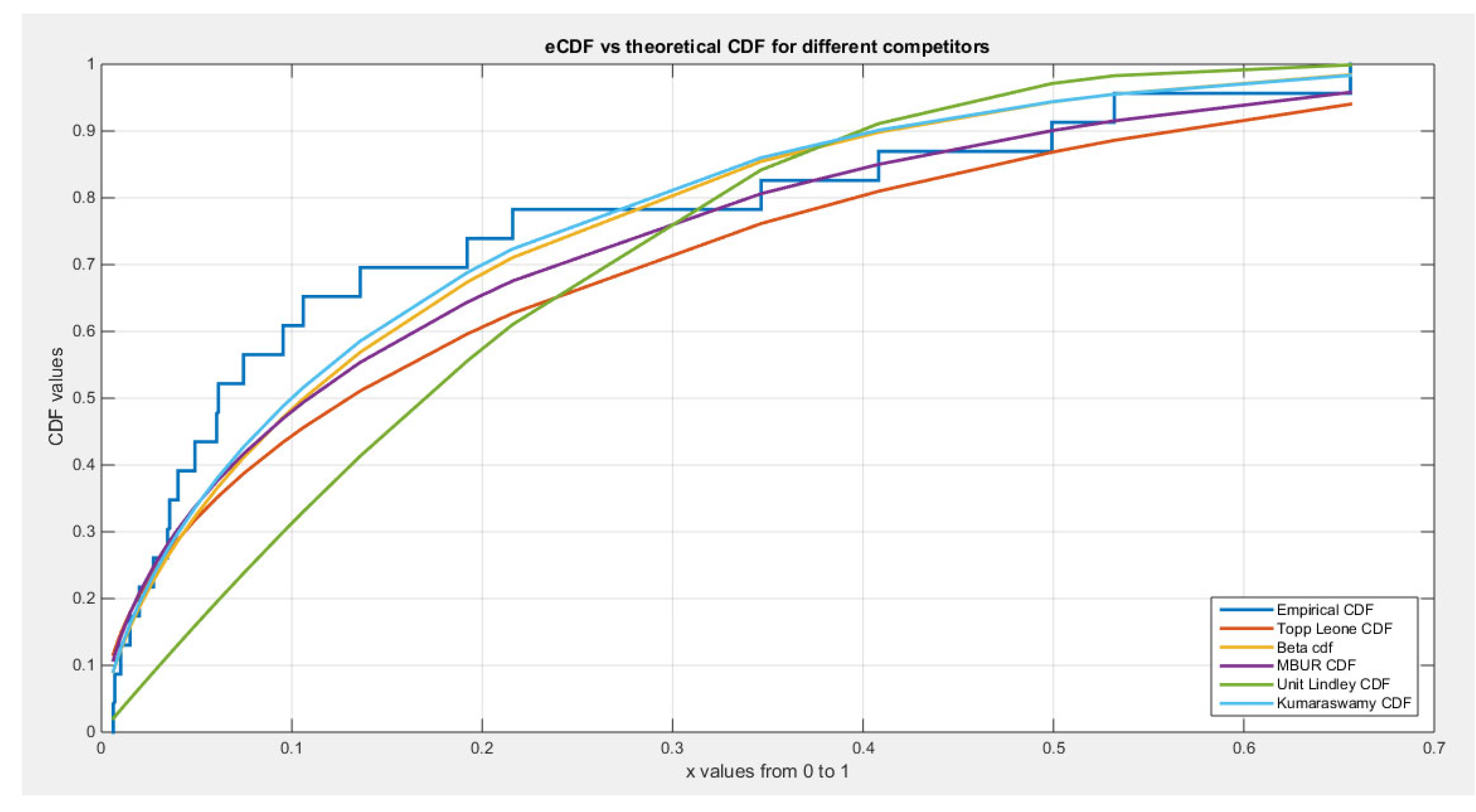
Analysis of above data sets and how do these sets fit the following distributions (unit distributions): Beta, Topp Leone, Unit Lindely, Kumaraswamy distributions is conducted and compared with the new distribution (MBUR Distribution). The tools for comparison are: -2LL, AIC, AIC corrected, BIC, Hannan Quinn Information Criteria (HQIC). Also K-S test is conducted with its value reported and the result of the H0 null hypothesis that assumes the data set follows the tested distribution otherwise reject the null. The P value for the test is also recorded. Figures of the empirical CDF (ecdf) and the theoretical CDF of the 5 distributions are illustrated. The values of the estimated parameters, their estimated variance and standard errors are reported.
First data set (Dwellings without basic facilities):
| Beta | Kumaraswamy | MBUR | Topp-Leone | Unit-Lindley | |||
| theta | 2.3519 | 0.2571 | 26.1445 | ||||
| Var | .0323 | .6661 | .0086 | .2424 | 0.023 | 0.0021 | 20.5623 |
| .6661 | 22.1589 | .2424 | 9.228 | ||||
| SE | 0.03227 | 0.01666 | 0.0272 | 0.0082 | 0.8144 | ||
| 0.8455 | 0.5456 | ||||||
| AIC | 161.5535 | 163.8979 | 147.3057 | 137.593 | 144.5918 | ||
| AIC¶correc | 161.982 | 164.3265 | 147.4436 | 137.7309 | 144.7297 | ||
| BIC | 164.4214 | 166.7659 | 148.7397 | 139.027 | 146.0258 | ||
| HQIC | 4.2816 | 4.2851 | 4.2611 | 4.2448 | 4.2567 | ||
| NLL | -78.7767 | -79.9489 | -72.6528 | -67.7965 | -71.2959 | ||
| K-S ¶Value | .2052 | .1742 | .2034 | .2818 | .3762 | ||
| H0 | Fail to reject | Fail to reject | Fail to reject | reject | reject | ||
| P-value | 0.1271 | 0.271 | 0.1336 | 0.0114 | 0.000189 | ||
Figure 11.
shows the eCDF vs. theoretical CDF of the 5 distributions for the 1st data set (Dwellings without basic facilities).
Figure 11.
shows the eCDF vs. theoretical CDF of the 5 distributions for the 1st data set (Dwellings without basic facilities).
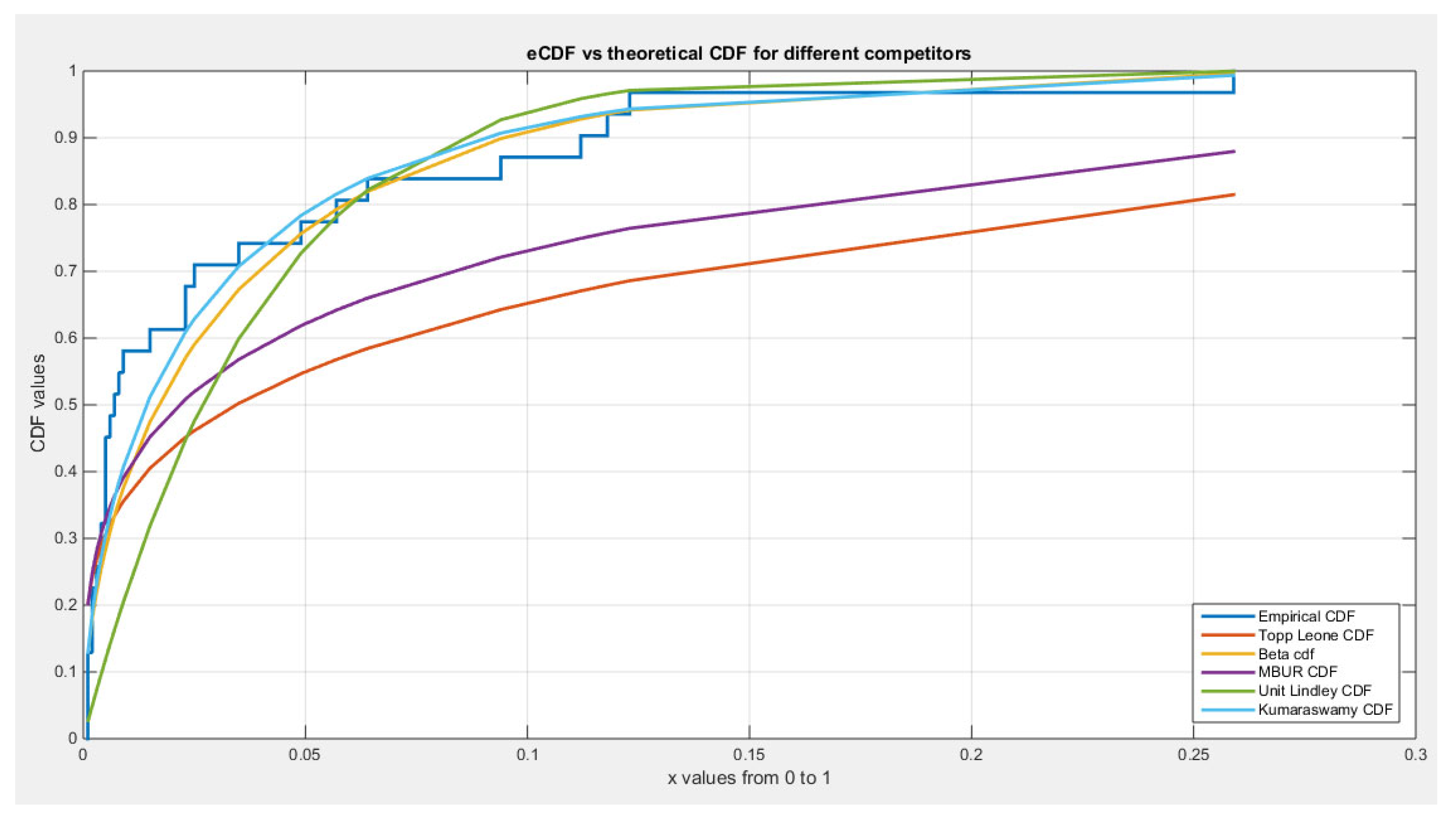
As shown from the analysis, 3 distributions better fit the data than the others; these are Beta, Kumaraswamy, and MBUR distributions. This is because the K-S test failed to reject the null hypothesis, H0, which hypothesized that the data being from the test distribution. MBUR had the lowest values of absolute values of NLL, AIC, corrected AIC, BIC, and HQIC values in comparison with the values obtained from the Beta and the Kumaraswamy distributions.
Second data set (Quality of support network):
| Beta | Kumaraswamy | MBUR | Topp-Leone | Unit-Lindley | |||
| theta | 0.3591 | 71.2975 | 0.1334 | ||||
| Var | 86.461 | 9.0379 | 15.7459 | 3.2005 | 0.0008 | 254.1667 | 0.00045 |
| 9.0379 | 1.0646 | 3.2005 | 1.0347 | ||||
| SE | 2.079 | 0.8873 | 0.0063 | 3.565 | 0.0047 | ||
| 0.231 | 0.2275 | ||||||
| AIC | 64.5056 | 64.7274 | 62.0790 | 60.6796 | 61.3746 | ||
| AIC¶correc | 65.2115 | 65.4333 | 62.3012 | 60.9018 | 61.5968 | ||
| BIC | 66.497 | 66.7188 | 63.0747 | 61.6753 | 62.3703 | ||
| HQIC | 3.9289 | 3.9299 | 3.9224 | 3.9159 | 3.9191 | ||
| NLL | -30.2528 | -30.3637 | -30.0395 | -29.3398 | -29.6873 | ||
| K-S ¶Value | .0974 | .0995 | .1309 | .1327 | .1057 | ||
| H0 | Fail to reject | Fail to reject | Fail to reject | Fail to reject | Reject to reject | ||
| P-value | 0.9416 | 0.9513 | 0.8399 | 0.4627 | 0.954 | ||
Figure 12.
shows the eCDF vs. theoretical CDF of the 5 distributions for the 2nd data set (Quality of support network). .
Figure 12.
shows the eCDF vs. theoretical CDF of the 5 distributions for the 2nd data set (Quality of support network). .
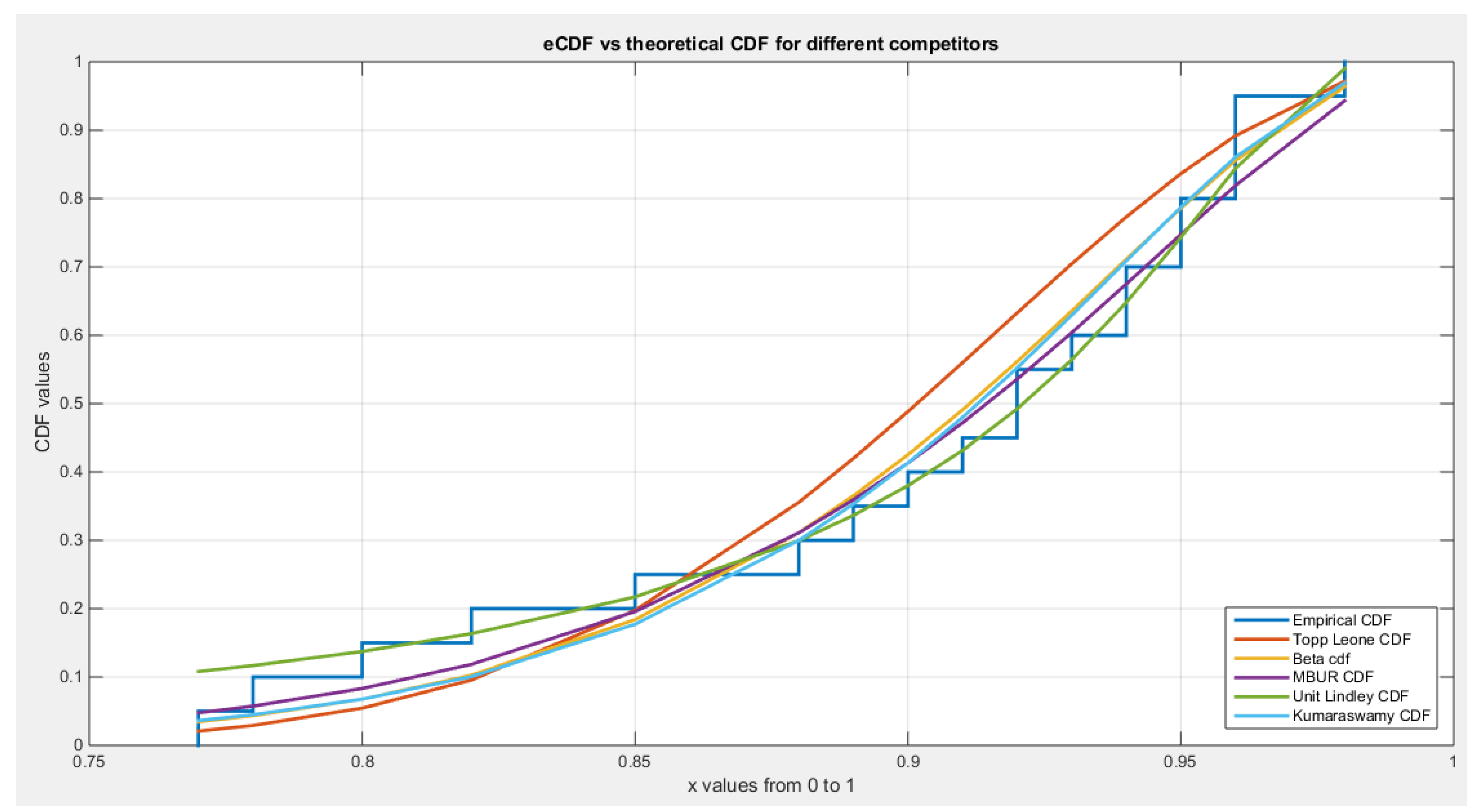
As shown from the analysis, 5 distributions fit the data well. This is because the K-S test failed to reject the null hypothesis, H0 ,which hypothesized that the data being from the test distribution. Topp-Leone had the lowest values of absolute values of NLL, AIC, corrected AIC, BIC, and HQIC values in comparison with the values obtained from the Unit-Lindley (which is the second next in ascending sort of the values) and the MBUR distributions (which is the third next in this ascending sort), followed by Beta then Kumaraswamy distributions.( in other words; ascending sort of the 5 distributions)
What is obvious in this analysis is that these metric values of MBUR distribution are comparable to those of Topp-Leone and Unit-Lindley, which denotes that the new distribution (MBUR) had accomplished a good job in fitting the data.
Third data set (Educational Attainment):
| Beta | Kumaraswamy | MBUR | Topp-Leone | Unit-Lindley | |||
| theta | 0.5556 | 13.4254 | 0.2905 | ||||
| Var | 3.4283 | 1.0938 | 1.3854 | 0.5232 | 0.0011 | 5.0067 | 0.0012 |
| 1.0938 | 0.416 | 0.5232 | 0.3234 | ||||
| SE | 0.3086 | 0.1962 | 0.0055 | 0.373 | 0.0058 | ||
| 0.1075 | 0.0948 | ||||||
| AIC | 54.6152 | 55.5937 | 52.8713 | 44.5725 | 60.9322 | ||
| AIC¶correc | 54.9789 | 55.9573 | 52.9890 | 44.6901 | 61.0498 | ||
| BIC | 57.7823 | 58.7607 | 54.4549 | 46.1560 | 62.5157 | ||
| HQIC | 4.0422 | 4.0471 | 4.0384 | 3.9916 | 4.0764 | ||
| NLL | -25.3076 | -25.7968 | -25.4357 | -21.2862 | -29.4661 | ||
| K-S ¶Value | .1453 | .1390 | .1468 | .2493 | .0722 | ||
| H0 | Fail to reject | Fail to reject | Fail to reject | Reject | Fail to reject | ||
| P-value | 0.2055 | 0.2411 | 0.1979 | 0.0062 | 0.8300 | ||
Figure 13.
shows the eCDF vs. theoretical CDF of the 5 distributions for the 3rd data set (Educational Attainment).
Figure 13.
shows the eCDF vs. theoretical CDF of the 5 distributions for the 3rd data set (Educational Attainment).
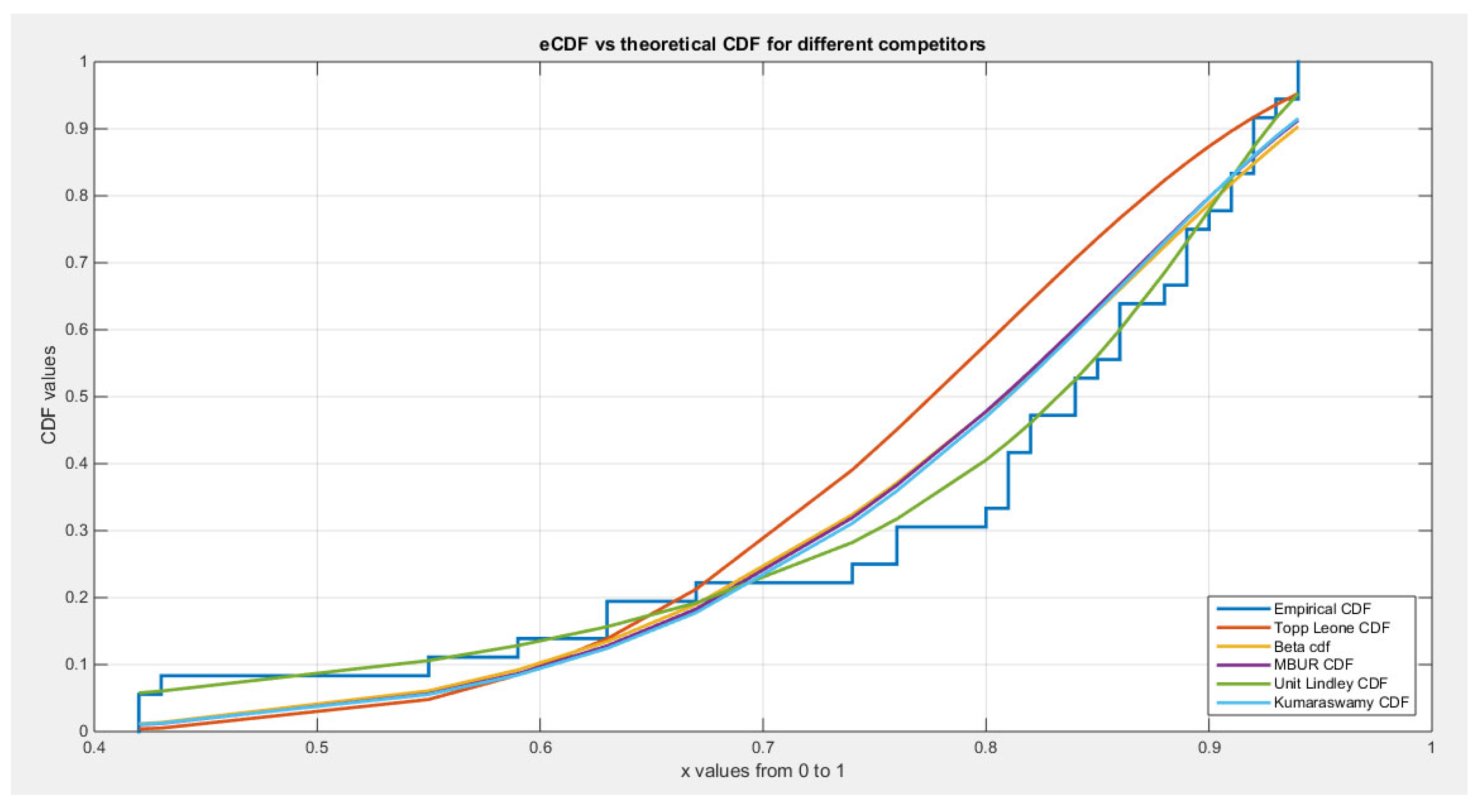
As shown from the analysis, 4 distributions fit the data well; all but not Topp-Leone which failed to fit the data well. This is because the K-S test failed to reject the null hypothesis, H0 , which hypothesized that the data being from the test distribution. MBUR distribution had the lowest values of absolute values of NLL, AIC, corrected AIC, BIC, and HQIC values in comparison with the values obtained from the Beta, Kumaraswamy and Unit-Lindley.
Fourth data set (Flood Data):
| Beta | Kumaraswamy | MBUR | Topp-Leone | Unit-Lindley | |||
| theta | 1.0443 | 2.2413 | 1.6268 | ||||
| Var | 7.22 | 7.2316 | 0.3651 | 2.8825 | 0.007 | 0.2512 | 0.0819 |
| 7.2316 | 8.0159 | 2.8825 | 29.963 | ||||
| SE | 0.6008 | 0.1351 | 0.0187 | 0.1121 | 0.0639 | ||
| 0.6331 | 1.2239 | ||||||
| AIC | 32.3671 | 55.5937 | 52.8713 | 44.5725 | 60.9322 | ||
| AIC¶correc | 33.073 | 30.6524 | 15.1455 | 16.985 | 16.5676 | ||
| BIC | 34.3586 | 31.938 | 15.9191 | 17.7585 | 17.3411 | ||
| HQIC | 3.7154 | 3.6893 | 3.456 | 3.4996 | 3.4902 | ||
| NLL | -14.1836 | -12.9733 | -6.4617 | -7.3814 | -7.1727 | ||
| K-S ¶Value | .2063 | .2175 | .3202 | .3409 | .2625 | ||
| H0 | Fail to reject | Fail to reject | Fail to reject | Reject | Fail to reject | ||
| P-value | 0.3174 | 0.2602 | 0.0253 | 0.0141 | 0.0311 | ||
Figure 14.
shows the eCDF vs. theoretical CDF of the 5 distributions for the 4th data set (Flood Data).
Figure 14.
shows the eCDF vs. theoretical CDF of the 5 distributions for the 4th data set (Flood Data).
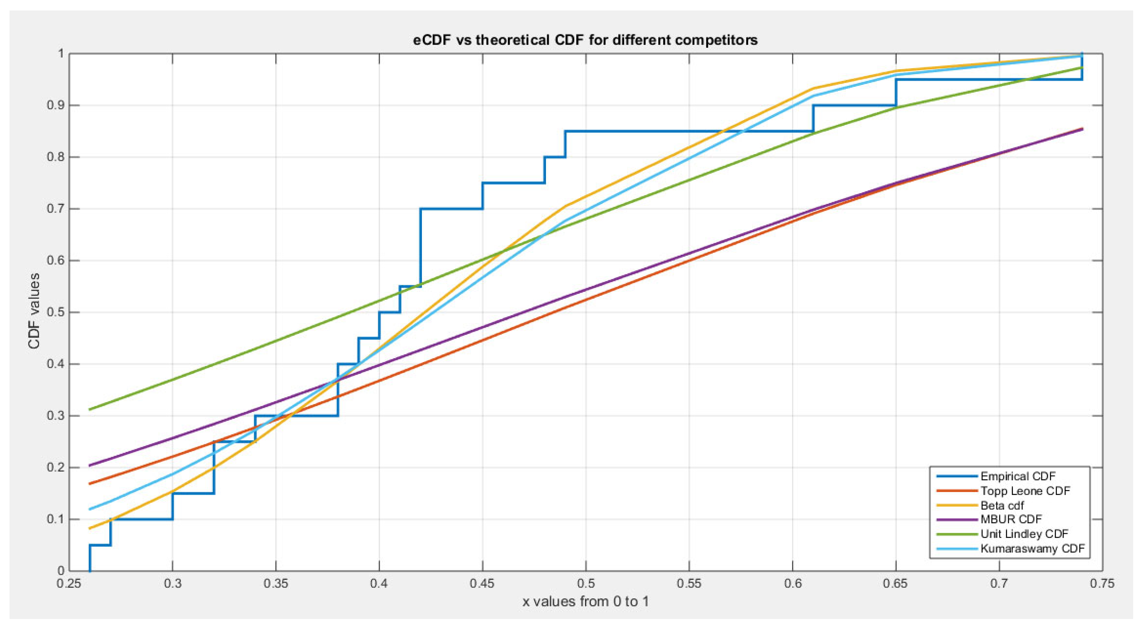
As shown from the analysis, 4 distributions fit the data well; all but not Topp-Leone which failed to fit the data well. This is because the K-S test failed to reject the null hypothesis, H0 , which hypothesized that the data being from the test distribution. MBUR distribution had the lowest values of absolute values of NLL, AIC, corrected AIC, BIC, and HQIC values in comparison with the values obtained from the Beta, Kumaraswamy and Unit-Lindley
What is obvious in this analysis is that these metric values of MBUR distribution are comparable to those of Topp-Leone, which denotes that the new distribution (MBUR) had accomplished a good job in fitting the data.
Fifth data set (Time Between Failures of Secondary Reactor Pumps):
| Beta | Kumaraswamy | MBUR | Topp-Leone | Unit-Lindley | |||
| theta | 1.7886 | 0.4891 | 4.1495 | ||||
| Var | 0.071 | 0.2801 | 0.0198 | 0.1033 | 0.018 | 0.0104 | 0.5543 |
| 0.2801 | 1.647 | 0.1033 | 0.9135 | ||||
| SE | 0.0555 | 0.0293 | 0.0279 | 0.0213 | 0.1552 | ||
| 0.2676 | 0.1993 | ||||||
| AIC | 44.0571 | 44.6592 | 41.862 | 39.5653 | 31.007 | ||
| AIC¶correc | 44.6571 | 45.2592 | 42.0525 | 39.7558 | 31.1975 | ||
| BIC | 46.3281 | 46.9302 | 42.9975 | 40.7008 | 32.1425 | ||
| HQIC | 3.8556 | 3.8598 | 3.8472 | 3.8303 | 3.7549 | ||
| NLL | -20.0285 | -20.3296 | -19.9310 | -18.7827 | -14.5035 | ||
| K-S ¶Value | 0.1541 | 0.1393 | 0.1584 | 0.1962 | 0.3274 | ||
| H0 | Fail to reject | Fail to reject | Fail to reject | Fail to Reject | Reject | ||
| P-value | 0.5918 | 0.7123 | 0.5575 | 0.2982 | 0.0107 | ||
Figure 15.
shows the eCDF vs. theoretical CDF of the 5 distributions for the 5th data set (Time Between Failures of Secondary Reactor Pumps).
Figure 15.
shows the eCDF vs. theoretical CDF of the 5 distributions for the 5th data set (Time Between Failures of Secondary Reactor Pumps).
As shown from the analysis, 4 distributions fit the data well; all but not Unit-Lindley which failed to fit the data well. This is because the K-S test failed to reject the null hypothesis, H0 , which hypothesized that the data being from the test distribution. Topp-Leone distribution had the lowest values of absolute values of NLL, AIC, corrected AIC, BIC, and HQIC values in comparison with the values obtained from the MBUR followed by Beta then the Kumaraswamy. (in other words in ascending sort)
Conclusion:
The need for new distribution to fit the data in many field of our life will help the scientists better understand the new emerging phenomena in a rapidly changing world and environment. This new MBUR is characterized by one parameter to be estimated. It has a well-defined CDF and a well-defined quantile function. It can accommodate wide variety of highly skewed data. The author is working to publish more properties of this distribution. I am also working on utilizing this distribution to be used in parametric quantile regression models that condition on the median rather than conditioning on the mean especially for data exhibiting high skewness. The generalized linear model conditioning on the mean can be used to analyze the data that are more or less symmetrical. I am also working on the Median Based Unit Weibull distribution (MBUW) distribution. I will compare it with this new MBUR distribution.
Future work:
The better fitting of data the better analysis can be obtained in many fields like regression, survival data analysis, reliability analysis, and time series analysis.
Declarations:
Ethics approval and consent to participate:
Not applicable.
Consent for publication:
Not applicable
Availability of data and material:
Not applicable. Data sharing not applicable to this article as no datasets were generated or analyzed during the current study.
Competing interests:
The author declares no competing interests of any type.
Acknowledgement:
Not applicable
References:
Author Contributions
AI carried the conceptualization by formulating the goals, aims of the research article, formal analysis by applying the statistical, mathematical and computational techniques to synthesize and analyze the hypothetical data, carried the methodology by creating the model, software programming and implementation, supervision, writing, drafting, editing, preparation, and creation of the presenting work.
Funding
No funding resource. No funding roles in the design of the study and collection, analysis, and interpretation of data and in writing the manuscript are declared
References
- Abdelmoezz, S., & Mohamed, S. M. (2021). The Kumaraswamy Lindley Regression Model with Application on the Egyptian Stock Exchange. Jurnal Matematika, Statistika Dan Komputasi, 18(1), 1–11. [CrossRef]
- Consul, P. C., & Jain, G. C. (1971). On the log-gamma distribution and its properties. Statistische Hefte, 12(2), 100–106. [CrossRef]
- Dumonceaux, R., & Antle, C. E. (1973). Discrimination Between the Log-Normal and the Weibull Distributions. Technometrics, 15(4), 923–926. [CrossRef]
- Eugene, N., Lee, C., & Famoye, F. (2002). BETA-NORMAL DISTRIBUTION AND ITS APPLICATIONS. Communications in Statistics - Theory and Methods, 31(4), 497–512. [CrossRef]
- Faradmal, J., Roshanaei, G., Mafi, M., Sadighi-Pashaki, A., & Karami, M. (2016). Application of Censored Quantile Regression to Determine Overall Survival Related Factors in Breast Cancer. Journal of Research in Health Sciences, 16(1), 36–40.
- Flemming, J. A., Nanji, S., Wei, X., Webber, C., Groome, P., & Booth, C. M. (2017). Association between the time to surgery and survival among patients with colon cancer: A population-based study. European Journal of Surgical Oncology (EJSO), 43(8), 1447–1455. [CrossRef]
- Grassia, A. (1977). ON A FAMILY OF DISTRIBUTIONS WITH ARGUMENT BETWEEN 0 AND 1 OBTAINED BY TRANSFORMATION OF THE GAMMA AND DERIVED COMPOUND DISTRIBUTIONS. Australian Journal of Statistics, 19(2), 108–114. [CrossRef]
- Gündüz, S., & Korkmaz, M. Ç. (2020). A New Unit Distribution Based On The Unbounded Johnson Distribution Rule: The Unit Johnson SU Distribution. Pakistan Journal of Statistics and Operation Research, 471–490. [CrossRef]
- Haq, M. A. U., Hashmi, S., Aidi, K., Ramos, P. L., & Louzada, F. (2023). Unit Modified Burr-III Distribution: Estimation, Characterizations and Validation Test. Annals of Data Science, 10(2), 415–440. [CrossRef]
- Johnson, N. L. (1949). Systems of Frequency Curves Generated by Methods of Translation. Biometrika, 36(1/2), 149–176. [CrossRef]
- Korkmaz, M. Ç., & Chesneau, C. (2021). On the unit Burr-XII distribution with the quantile regression modeling and applications. Computational and Applied Mathematics, 40(1), 29. [CrossRef]
- Kumaraswamy, P. (1980). A generalized probability density function for double-bounded random processes. Journal of Hydrology, 46(1–2), 79–88. [CrossRef]
- Maya, R., Jodrá, P., Irshad, M. R., & Krishna, A. (2024). The unit Muth distribution: Statistical properties and applications. Ricerche Di Matematica, 73(4), 1843–1866. [CrossRef]
- Mazucheli, J., Maringa, A. F., & Dey, S. (2019). Unit-Gompertz Distribution with Applications. Statistica, Vol 79, 25-43 Pages. [CrossRef]
- Mazucheli, J., Menezes, A. F. B., & Chakraborty, S. (2019). On the one parameter unit-Lindley distribution and its associated regression model for proportion data. Journal of Applied Statistics, 46(4), 700–714. [CrossRef]
- Mazucheli, J., Menezes, A. F. B., & Dey, S. (2018). Improved maximum-likelihood estimators for the parameters of the unit-gamma distribution. Communications in Statistics - Theory and Methods, 47(15), 3767–3778. [CrossRef]
- Mazucheli, J., Menezes, A. F. B., Fernandes, L. B., De Oliveira, R. P., & Ghitany, M. E. (2020). The unit-Weibull distribution as an alternative to the Kumaraswamy distribution for the modeling of quantiles conditional on covariates. Journal of Applied Statistics, 47(6), 954–974. [CrossRef]
- Modi, K., & Gill, V. (2020). Unit Burr-III distribution with application. Journal of Statistics and Management Systems, 23(3), 579–592. [CrossRef]
- Mohamed, M.r., A.A. ElSheikh, Naglaa A. Morad, Moshera A.M. Ahmed . Log-Beta Log-Logistic Regression Model. Retrieved September 24, 2024, from https://core.ac.uk/reader/249334660.
- suprawhardana. (1999). Suprawhardana, M.S., Prayoto, S.: Total time on test plot analysis for mechanical components of the RSG-GAS reactor. At. Indones. 25(2), 81–90 (1999). 25(2),81-90(1999), 25(5), 81–90.
- Tadikamalla, P. R. (1981). On a family of distributions obtained by the transformation of the gamma distribution. Journal of Statistical Computation and Simulation, 13(3–4), 209–214. [CrossRef]
- Tadikamalla, P. R., & Johnson, N. L. (1982). Systems of frequency curves generated by transformations of logistic variables. Biometrika, 69(2), 461–465. [CrossRef]
- Topp, C. W., & Leone, F. C. (1955). A Family of J-Shaped Frequency Functions. Journal of the American Statistical Association, 50(269), 209–219. [CrossRef]
- Xue, X., Xie, X., & Strickler, H. D. (2018). A censored quantile regression approach for the analysis of time to event data. Statistical Methods in Medical Research, 27(3), 955–965. [CrossRef]
Figure 1.
pdf of Median Based Unit Rayleigh ( MBUR) distribution.
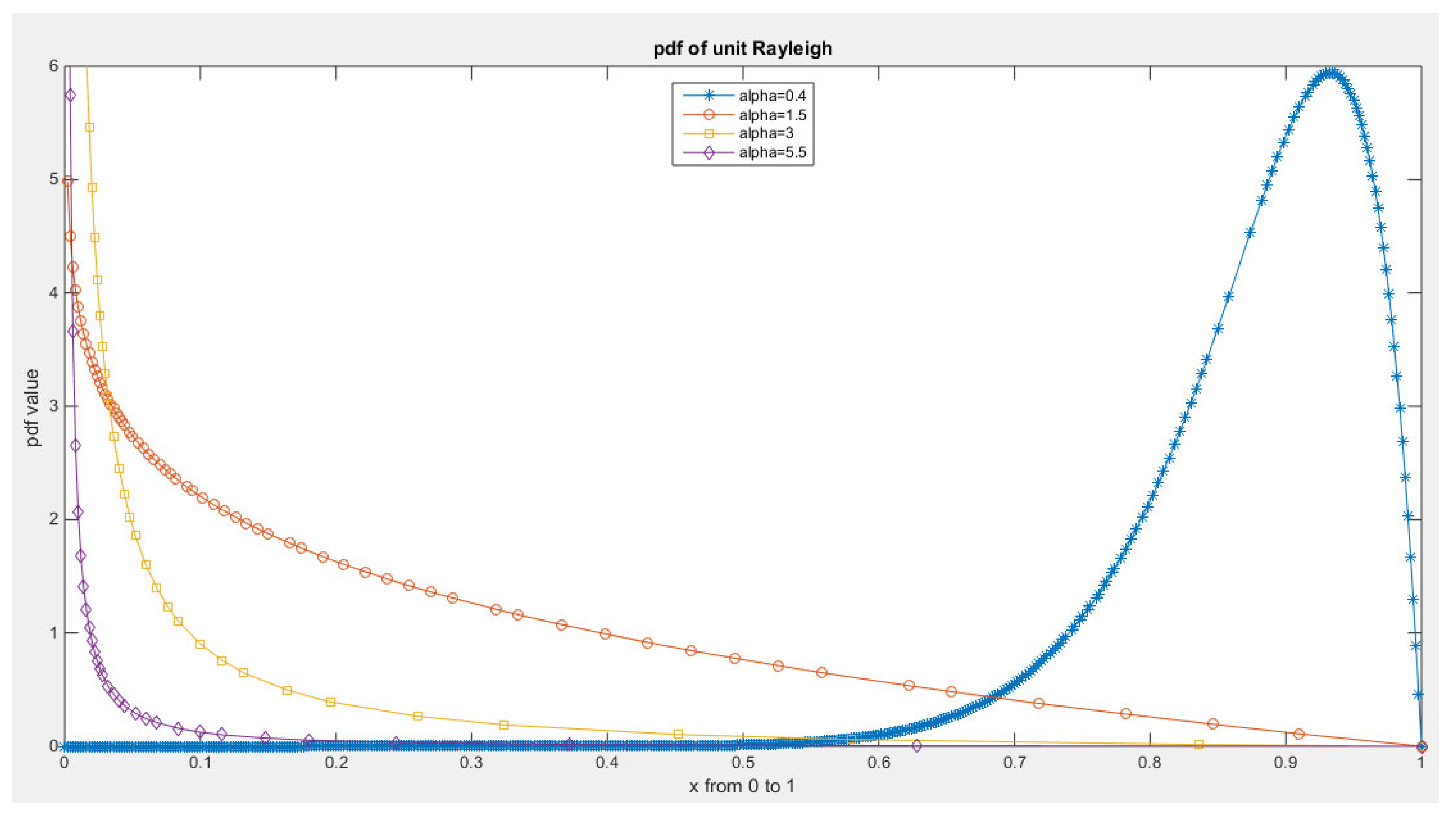
Figure 2.
pdf of Median Based Unit Rayleigh ( MBUR) distribution.
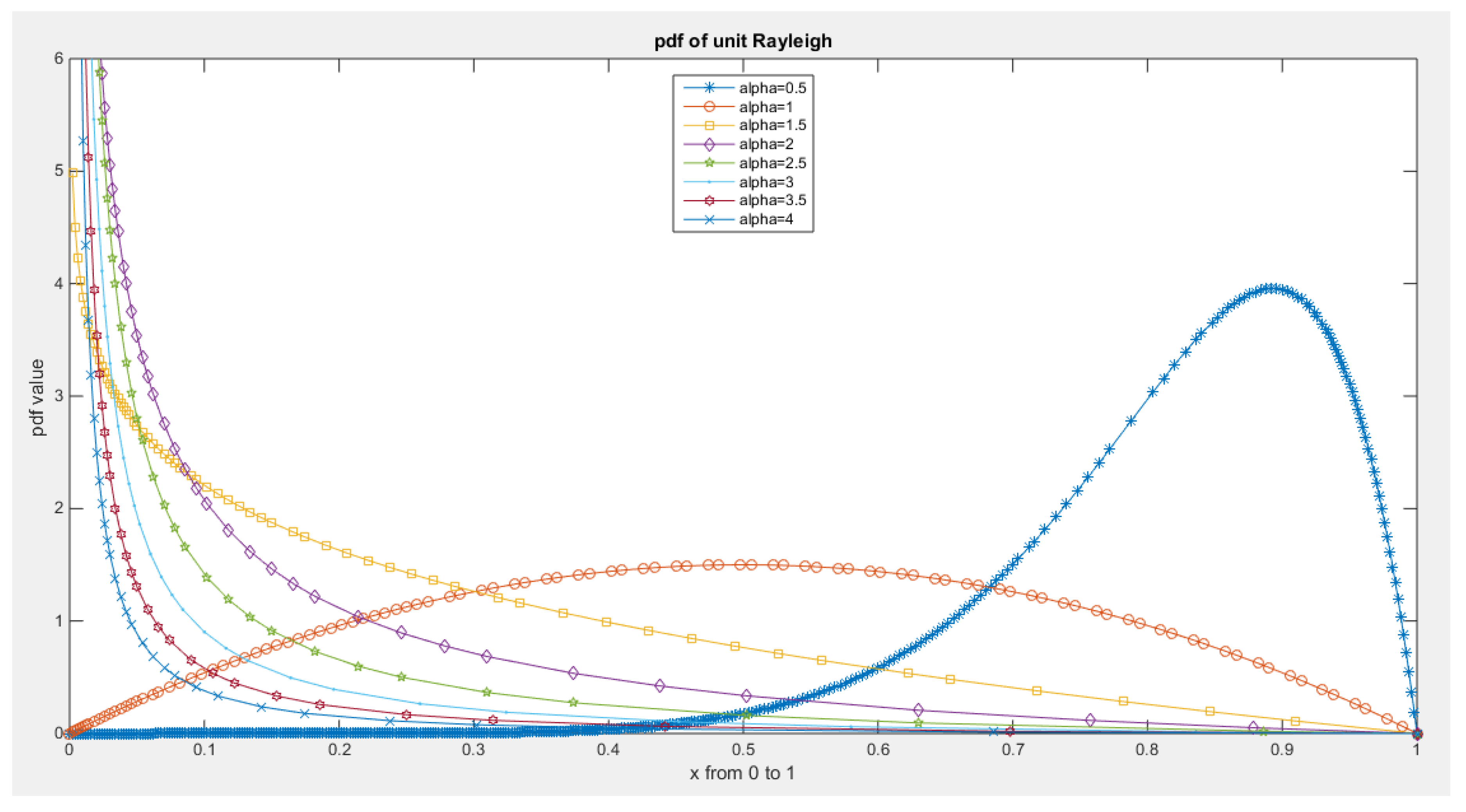
Figure 3.
CDF of Median Based Unit Rayleigh ( MBUR ) Distribution.
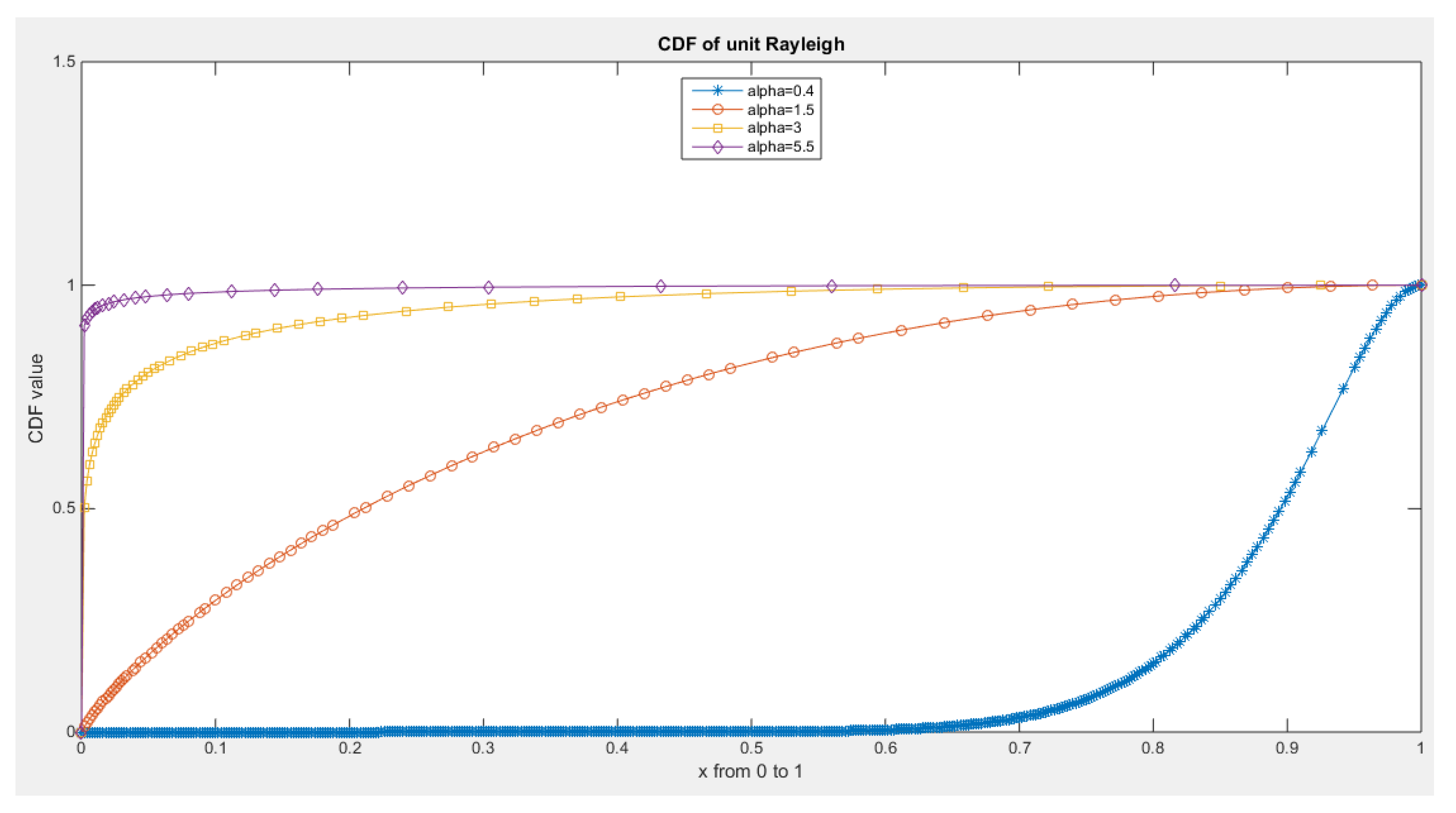
Figure 4.
CDF of Median Based Unit Rayleigh ( MBUR ) Distribution.
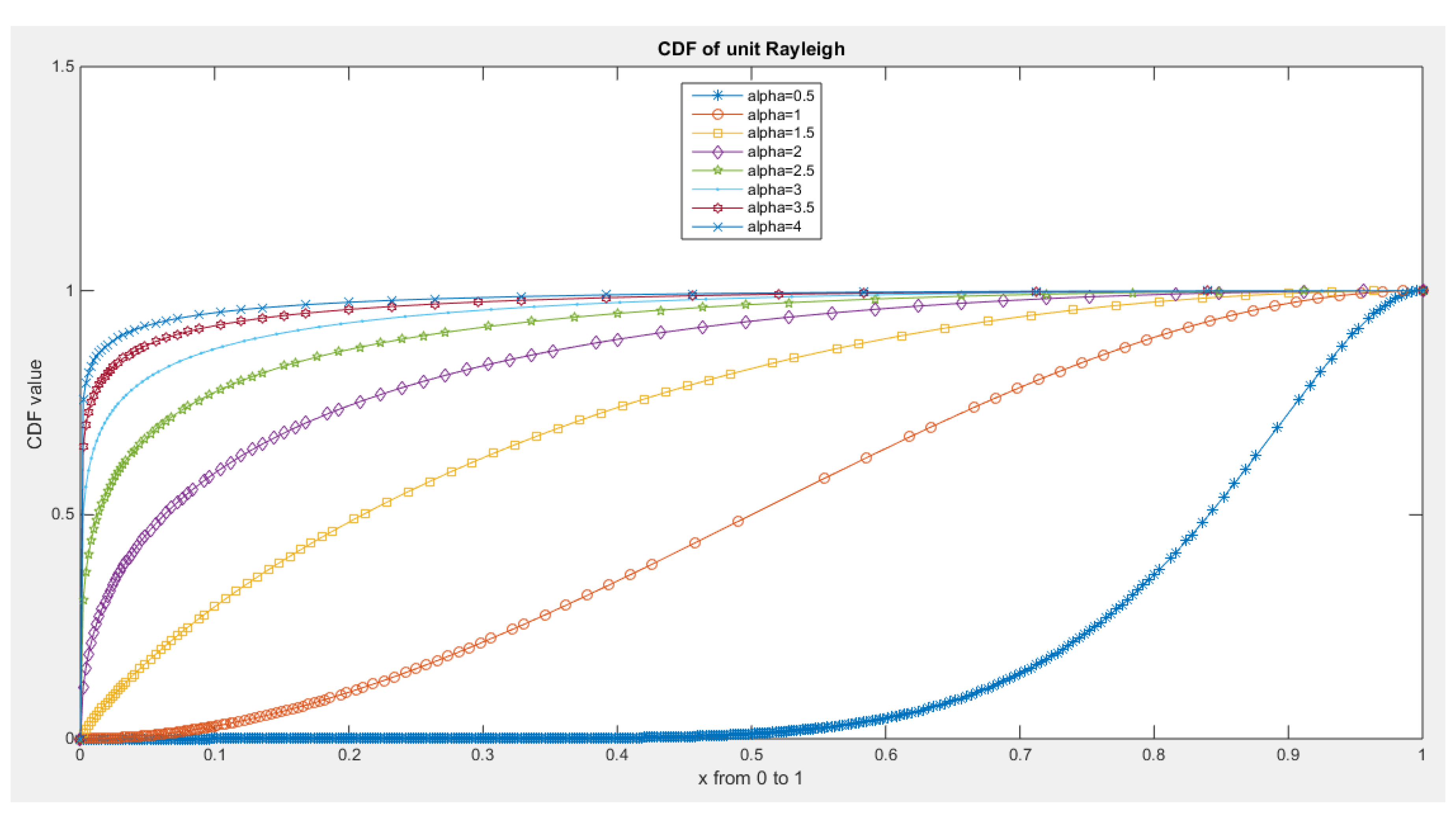
Figure 5.
survival function of MBUR Distribution.
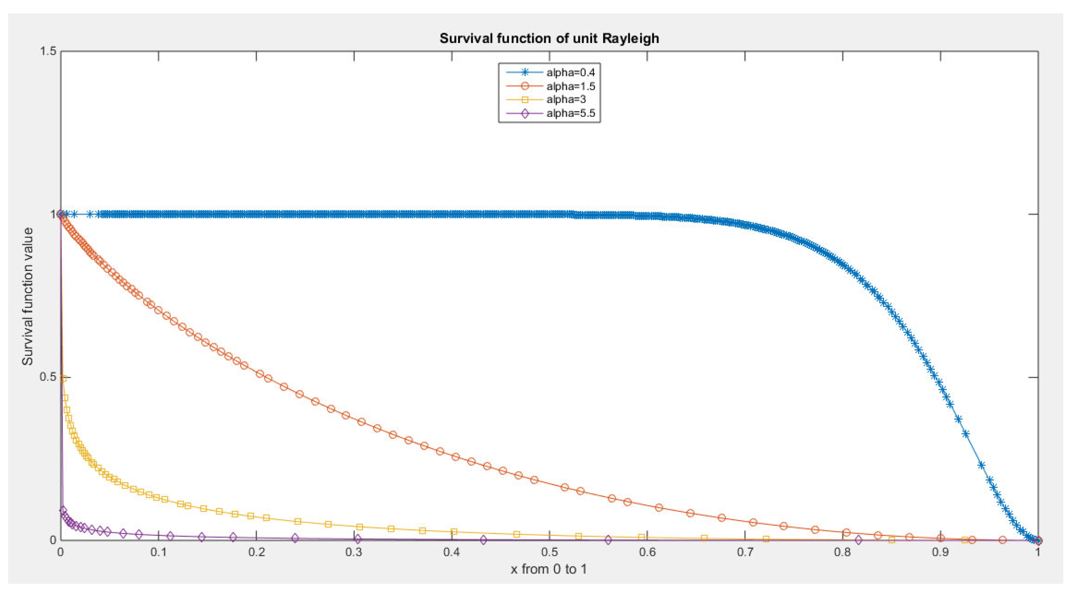
Figure 6.
survival function of MBUR Distribution.

Figure 7.
hazard rate function of MBUR Distribution.
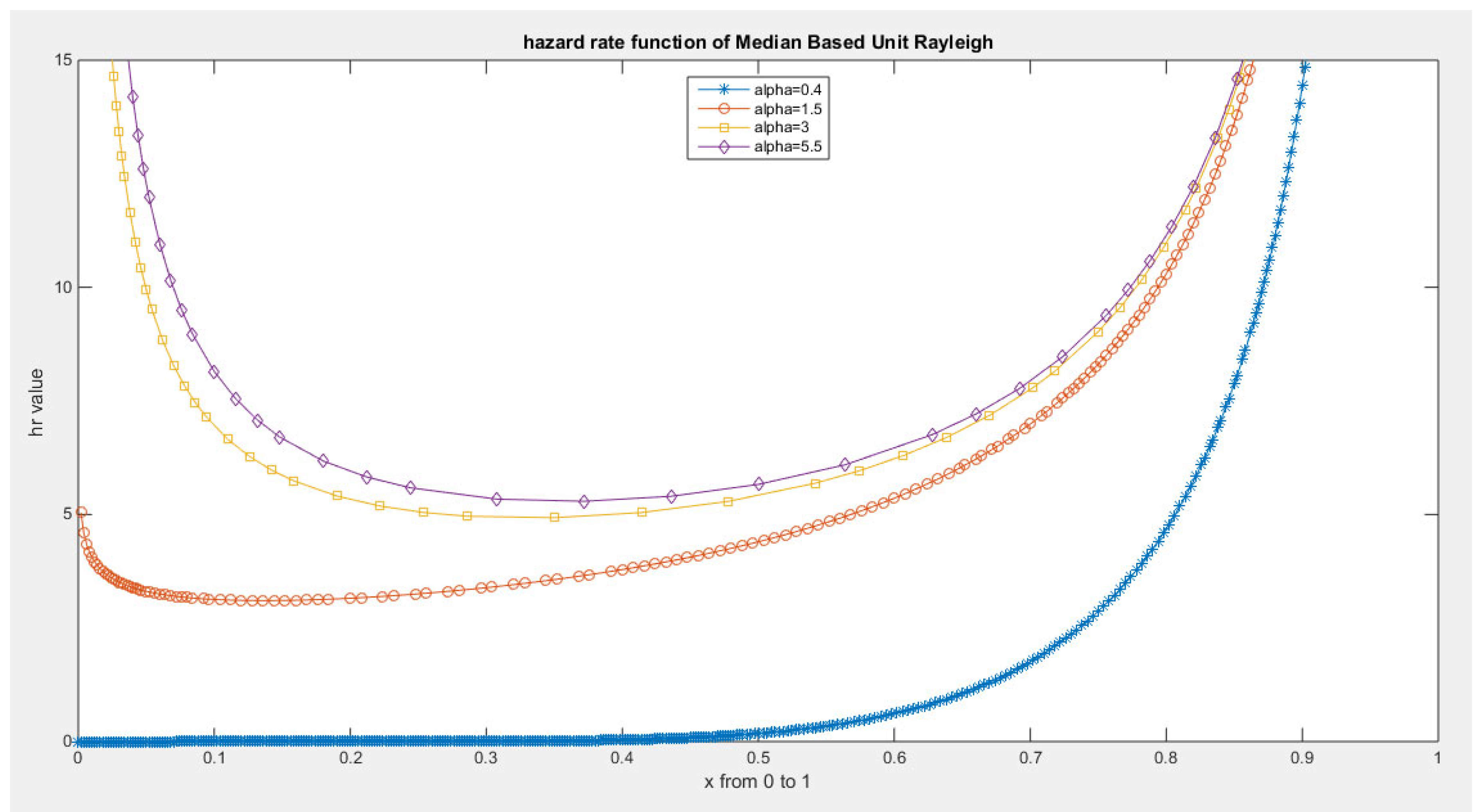
Figure 8.
hazard rate function of MBUR Distribution.
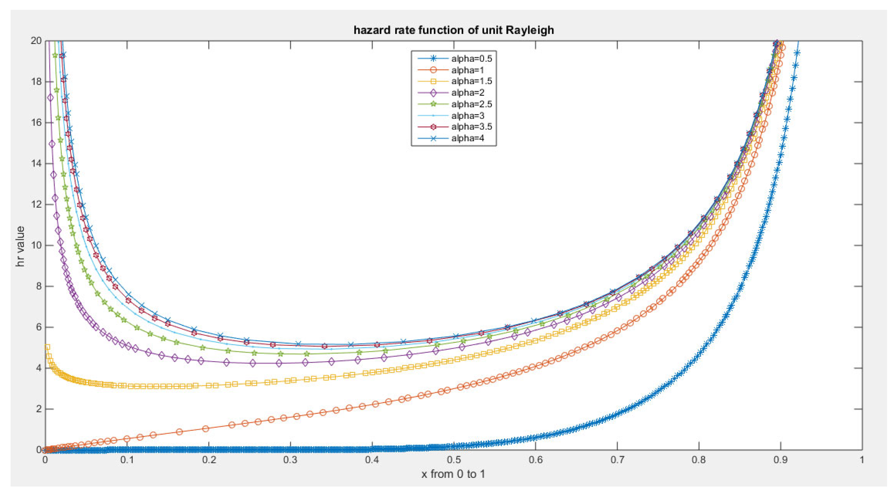
Figure 9.
reversed hazard rate function of MBUR Distribution.
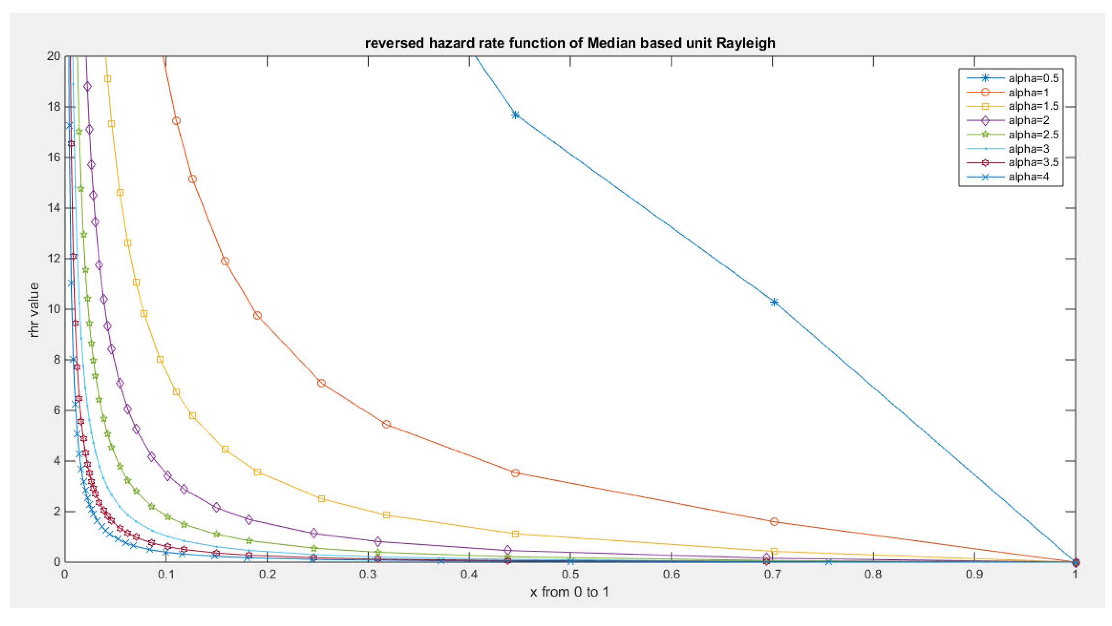
Figure 10.
the variance and different coefficients with different levels of alpha.
Disclaimer/Publisher’s Note: The statements, opinions and data contained in all publications are solely those of the individual author(s) and contributor(s) and not of MDPI and/or the editor(s). MDPI and/or the editor(s) disclaim responsibility for any injury to people or property resulting from any ideas, methods, instructions or products referred to in the content. |
© 2024 by the authors. Licensee MDPI, Basel, Switzerland. This article is an open access article distributed under the terms and conditions of the Creative Commons Attribution (CC BY) license (http://creativecommons.org/licenses/by/4.0/).
Copyright: This open access article is published under a Creative Commons CC BY 4.0 license, which permit the free download, distribution, and reuse, provided that the author and preprint are cited in any reuse.


