1. Introduction
This article solves the problem of assessing the accuracy, stability and reproducibility of exemplary frequency generators that serve as frequency and time standards at a new level of understanding, for which the theoretical and practical aspects of their certification are considered.
Estimation of frequency standards is the most important task of fundamental metrology, since through frequency and time one can also specify a measure of extent, which is a length standard, which is what is currently used [
1,
2,
3,
4,
5,
6,
7,
8,
9,
10,
11,
12,
13,
14,
15,
16,
17,
18,
19,
20,
21,
22,
23,
24,
25,
26,
27,
28,
29,
30]. Thus, measures of time and space are directly related to frequency standards, so their certification is extremely relevant.
The author supervised the development of metrological tools for assessing the stability of laser frequency standards, the generation frequency of which is usually high, for example, about 89 THz. Two identical lasers are used to form a difference frequency, which carries information about the result of the total deviation of the frequencies of these lasers from its ideal value, the contribution to the difference frequency from each laser is considered statistically independent, which allows certifying such frequency standards in accordance with the theory stating that the resulting variance of the difference frequency is equal to twice the frequency variance of each of the stabilized lasers. Based on the experience and theoretical and experimental studies of the author, the article considers the problems of applying the Allan function and interpreting this measure in relation to the properties of the created prototypes of the laser frequency standard. This article does not consider the structure and theory of noise occurrence, as well as laser stabilization methods, but focuses only on experimental methods for studying the stability of frequency standards and on the interpretation of the obtained experimental materials.
Any random variable can and should be assessed by its statistical characteristics—mathematical expectation, variance, and so on. As a rule, those who use metrological tools focus on parameters such as absolute error or relative error . Each of these two types of errors is maximum , , statistical average , and mathematical expectation, that is, offset , . The maximum error characterizes the maximum error value when using this metrological tool. The average statistical error is the most probable measurement error based on the random distribution of errors. Displacement is the mathematical expectation of the deviation of a measurement result from the true value. As a rule, developers strive to create a metrological tool with zero offset, but this, strictly speaking, is unattainable. The absolute value of each of these three types of error is expressed in measured units, and the relative value is the ratio of the absolute error to the measured value, or to the maximum possible value when using this measuring instrument, or in some cases to some specially selected value. Relative error is a value without units of measurement.
Users, as a rule, focus precisely on these indicators of the accuracy of any measuring instrument.
For example, if we have a stable frequency generator based on temperature-stabilized quartz, then its maximum relative error, according to the promised characteristics from the best manufacturers, can be of the order of . This means that, for example, if a given generator generates a frequency value that, according to the data sheet, is equal to , then the absolute maximum error is the actual frequency value must lie within . In this case, if you use such a generator to clock an electronic clock, then when measuring sufficiently large time intervals, the specified error is predominant, that is, the error in measuring any large time interval will be equal to For example, an error equal to one second will be when measuring a time interval equal to about 316.9 years. Accordingly, in 1 year such a clock will accumulate an error of only approximately 3.15 milliseconds. Certification of quartz generators is not a scientific problem, since there are more accurate generators. Therefore, it is sufficient to compare the frequency of such a generator with the frequency of a more accurate generator to describe all types of its errors, including the absolute error.
The indicated high measurement accuracy turns out to be insufficient for modern measurements; the tasks of developing time standards that would be described by accuracy characteristics at the level of and even are relevant , and for a number of future tasks they are already talking about the need to have “atomic clocks” or “laser clocks” with an error at the level , in particular, for the task of detecting gravitational waves created by the Crab Nebula using an interferometer formed by three satellites in geostationary orbits, the distance between which is maintained with a relative error within the specified limits.
Despite the fact that there are reports that technical solutions have been tested confirming the error of the generated frequency at the specified level, that is, with a value of the order of magnitude,
one should be extremely careful with these messages, since they do not give the characteristics mentioned above, but the so-called Allan function [
1,
2,
3,
4,
5,
6,
7,
8,
9,
10,
11,
12,
13,
14,
15,
16,
17,
18,
19,
20,
21,
22,
23,
24,
25,
26,
27,
28,
29,
30], which was introduced by Allan in publication [
1], which is far from the same thing.
Not all publications, reports and dissertations differentiate such characteristics as accuracy and stability correctly enough. For secondary frequency standards, accuracy is determined by comparison with primary standards, but this method is not applicable when certification of laser or atomic frequency standards is required, i.e., primary standards or devices that claim such status. In this case, the stability of such devices is investigated, after which a device with higher stability is considered a device with higher accuracy, which, of course, is not true, but there is simply no other way to certify primary standards. Therefore, the study of the stability of primary standards or their prototypes is a fundamental physical problem.
This article raises the question of how related indicators such as the Allan function [1, 2] are with indicators such as frequency error and irreproducibility, and to what extent this instability indicator can be used as an indicator of frequency generation error.
It should also be noted that there are other stability estimates, such as the modified Allan variance [
31], Hadamard variance [
32], modified Hadamard variance, and other stability indices [
32]. They are used to better evaluate frequency stability, but not its accuracy. Since Allan variance is accepted by the IEEE community as the main indicator of frequency generator stability [
2], other indices are not as important, are mentioned and used orders of magnitude less frequently, and therefore a discussion of these indices is beyond the scope of this article.
Many groups developing laser and atomic frequency standards report their research results using Allan variance plots without providing any other characteristics, for example [
33]. This may be due to the fact that primary frequency standards cannot be assessed for accuracy, since they are a priori assumed to be better than all other reference oscillators. An approach used to assess them is to assess the stability of such oscillators, and if their stability is much higher than that demonstrated by the frequency standards used, then such devices are considered to be replacements for primary frequency standards. Thus, when creating primary frequency standards, the accuracy and stability characteristics are treated as equivalent, although this is, of course, a mistake. This approach also applies to potential prototypes of primary standards and, in general, to any newly created oscillator for which increased accuracy is claimed or promised. Thus, in fact, the Allan parameters replace the certification of frequency standards and reference oscillators for new atomic clocks, which can be traced even in the technical specifications for the development of such devices. The author believes that this is wrong, this article aims to clarify this situation based on theoretical concepts and with confirmation of the modeling results.
2. Statement of the Problem and Problems
It is extremely important to analyze the traditional measure of stability of generators, such as the Allan function [1, 2], to evaluate the validity of statements about how it changes in the areas of the argument and , to assess the admissible form of asymptotes of this function in these areas, both from the standpoint of the reliability of the assumptions used, and from the position of accepting such assumptions and applying them to evaluate frequency and time standards, to formulate criteria for comparing such devices according to their user characteristics.
The fact is that, along with the characteristics of the frequency formation error, such a generally accepted characteristic as “stability” is used, a value associated with “instability”, a value that is easier to describe numerically. To understand the problem, we introduce two additional characteristics: instability and irreproducibility of the generated frequency.
Frequency instability is determined by frequency deviations from a certain value, accepted and called the starting value. For example, if at some point in time the frequency difference of two identical generators generating a frequency of approximately 100 THz turned out to be 100 Hz, then this value can be conditionally taken as the starting value. If this frequency remained strictly the same for some time, then in this ideal case the instability, that is, the deviation from this frequency, should be characterized as zero. But strictly zero instability does not exist, any frequency has some drift. For example, if the difference frequency deviates by an amount corresponding to one unit of the 16th order, that is, by 0.01 Hz, then this can be recorded even with a conventional frequency meter. Thus, measurements in the radio frequency region of the difference frequency allow certifying highly stable generators generating an extremely high frequency, and recalculating these measurement results into units of extremely small frequency instability. Thus, historically, such measurements were carried out, but in order to measure frequency with an error of about 0.01 Hz, it is necessary to have measuring devices with a smaller error. A conventional frequency meter of the counting type, for example, has an error in measuring frequency over a period of 1 s of about 1 Hz, i.e., an error of less than 0.001 Hz will be achieved only by averaging the frequency over a time interval of more than 1000 s.
The error of frequency reproduction is called irreproducibility. For example, in the case considered above, if two identical generators, which due to their structure and operating principle should generate the same frequency, nevertheless generate two different frequencies, which, as determined experimentally, differ by 100 Hz, then this difference somehow characterizes the starting irreproducibility of the frequency. For example, it can be assumed that each of the standards will deviate from the true value (which the ideal standard should generate) equally, but independently of each other. For this deviation, it is possible to introduce not only the starting value, but also statistical characteristics, for example, in the presence of an ensemble of frequency standards, it is possible to obtain a set of frequency values, for which it is possible to determine the average and specific deviations of each of them. Naturally, the average frequency value will be equal to the sum of all values, divided by the number of such generators, and the deviation of each generator from this average is the difference between the actual value of the frequency generated by it and this average. Naturally, the sample average is not identical to the global average, but it can to some extent serve as an estimate of this value. If it is impossible to investigate an ensemble of generators (as is almost always the case), then at least two generators have to be investigated, considering the ergodic property to be valid, according to which averaging in time is to some extent related to averaging over time. This hypothesis is never proven by anyone, but is simply accepted due to the lack of another way to investigate the accuracy of primary frequency standards. The measure of irreproducibility, like the measure of instability, depends not on one argument, but on many. For example, instability can be estimated at different values of the averaging time. The same can be true for such a measure as instability, since frequency measurement is always carried out at some time intervals and the result always depends on the duration of this interval, and also at different intervals of the same duration the result will be different.
In this case, “stability” can be characterized by the inverse of relative instability, and, accordingly, reproducibility should be calculated by the inverse of relative irreproducibility.
The characteristic “instability”, which we denote, will characterize the relative deviation of the generated value from the starting value.
Consider, for example, some function that varies over time. If , that is, this function does not change over time at all, then the instability will be equal to zero: .
It can also be argued that for , where is a constant coefficient, , since the specified function characterizes only the relative departure of the value from the initial value . Thus, changing the frequency scale will not make any contribution to this characteristic.
In addition, if two random variables differ only in a constant displacement, for example, , then the instability of the second value in comparison with the instability of the first value will differ only due to the difference in the value to which the absolute instability will be attributed. If at the same time , then practically the difference will be in the sign of the order of instability (and this is usually above the 12th sign of magnitude), and the value of “instability” is estimated with an error of a few percent, or even with an accuracy of up to an order of magnitude, for example, “three units of the 13th sign.” Consequently, a constant frequency shift has practically no effect on the frequency instability indicator, as well as on its inverse frequency stability indicator.
Let’s consider a generator that generates a frequency that changes relatively little over time. . These small changes are the basis for calculating the stability characteristics of the generated frequency. Moreover, if the generated frequency differs from the value that we require, or that we attribute to this generator by the amount of error , then the instability characteristic of this frequency does not depend in any way on this value. In other words, .
Let’s discuss how this will manifest itself if the generator we use based on such characteristics is used to measure a certain period of time. Let us assume that the instability of the generator, expressed by some numerical value, is equal to , where is the averaging time, which in this case is equal to, say, one year. This means that if we will use such clock to measure the interval of time equal to 1 year, then the maximal accumulated error of the measuring will be about 3.15 milliseconds. But in this case we should not talk about the error in measuring time, but about the deviation of the measurement result from the value that we would have received if instead of this generator we had used another generator whose generation frequency at time t = 0 would completely coincide with the frequency of this generator, and then throughout the year it would not change at all. But if, for example, the frequency of a given generator differs from the one that it should generate by some amount, this stability assessment will not increase in any way, even if this error is, for example, 0.001%. In this case, over 1 year, an error in time measurement will accumulate equal to 8 hours 46 minutes. So, as we see, the discrepancy between the generated frequency and the value that is required is a cut-off flaw of the generator for using it as a standard for units of time or frequency, but an indicator that takes into account only the stability of the generated frequency does not take this discrepancy into account.
Let us now consider such a characteristic as irreproducibility, which is proposed to be denoted by the value . The point is that if we turn on the same generator at different times, then the value of the frequency that it generates at the moment it is turned on, at the moment from which we begin to measure the stability of its frequency, will have a random deviation. The measure of this deviation will be irreproducibility. The difference in the results of two experiments will give a single deviation of the starting values, and the statistical characteristics of these differences will give a statistical characteristic of irreproducibility. Another interpretation, more statistically correct, can be formulated based on the concept of an ensemble of generators. If there are several strictly identical generators that we turn on approximately simultaneously, then the difference in the starting values and the frequencies they generate characterize the single values of this random variable, and the statistics of this random variable will characterize irreproducibility. We can talk about the mathematical expectation of this quantity, the mean square of this quantity, and the square root of the mean square of this quantity.
For example, we can call the maximum deviation over the entire ensemble maximum irreproducibility:
The relative irreproducibility in this case will be determined by the ratio of this value to the average value, and since it does not change significantly, since we are still discussing exemplary frequency generators, we can use the starting value as the value in relation to which the relative instability is calculated:
And now it makes sense to turn to the characteristic of “accuracy” or “stability” of frequency standards [
1], which is approved by the IEEE community [
2] and has been used as the main one for many decades [
1,
2,
3,
4,
5,
6,
7,
8,
9,
10,
11,
12,
13,
14,
15,
16,
17,
18,
19,
20,
21,
22,
23,
24,
25,
26,
27,
28,
29,
30]. We are talking about the Allen function [1, 2].
3. Generally Accepted Characteristic of Stability of Frequency Standards
A generally accepted numerical characteristic of the relative instability of modern frequency standards is a function depending on the averaging time τ, which is called two-sample Allen variance [1, 2]. It is determined by the following relationship:
Here, angle brackets denote the statistical average over an ensemble of pairs of measurements, which in the experiment is replaced by averaging over the set of all values i, the values , mean the average frequency values at adjacent time intervals lasting τ seconds, with zero “dead time” D = 0 between them. The literature also sometimes misses the two in the argument, indicating that it is a two-sample variance, so the simplified notation is used .
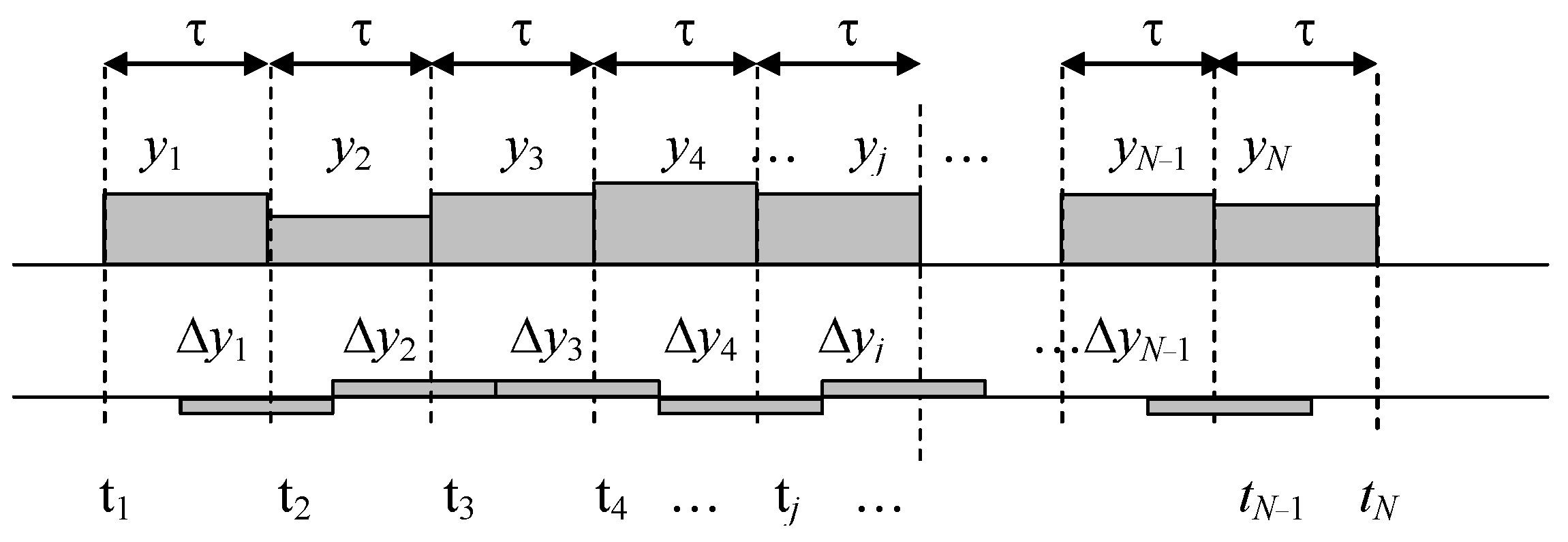
Figure 1 shows how the time intervals are located at which the average frequency values should be taken.
Evaluation of the frequency stability of frequency primary standards, that is, model generators, is carried out using a technique based on measuring the difference frequency of two completely identical generators.
The top chart of
Figure 1 shows the average frequency values over several adjacent intervals. Within these intervals, the frequency also changes in some way, but the average value is equal to the area formed by the figure, the lower boundary of which is a segment of the time axis of length τ, the upper boundary is the function y(t) strictly above this segment, and the left and right boundaries are vertical lines. Conventionally, these values can be represented by rectangles, the height of which is equal to the average frequency value in this segment. Then the differences between subsequent measurement results will be equal to the difference in the areas of these rectangles, as shown in the bottom diagram of
Figure 1.
This function is depicted, as a rule, on a double logarithmic scale, the right one often corresponds to an increase in the averaging time, and the left one to a decrease with a tendency to zero, with the zero value lying at minus infinity.
The main problems arise at and at : in both cases, the value of the Allen function obtained experimentally on some part of these axis segments open on one side increases. This was the reason for the spread of the opinion that the behavior of this function almost always in these extreme regions can be approximated by oblique asymptotes, that is, the hypothesis that the values of the Allen function actually increase unlimitedly for most real generators on open intervals corresponding to and .
Thus, Ryutman claims that a graph
on a double logarithmic scale consists of straight line segments, the slope of which he further determines [
2]. He states that for frequency flicker noise the two-sample variance
is independent of
; The corresponding section of the current on the graph is often called flicker flattening.
He also carries out all further reasoning in relation to the two-sample variance (3), while in the literature it is almost always constructed on a double logarithmic scale not the variance (3), but the square root of this variance, which is usually called the Allen function:
As a rule, this value is given in relative units, referred to the average frequency of the generator.
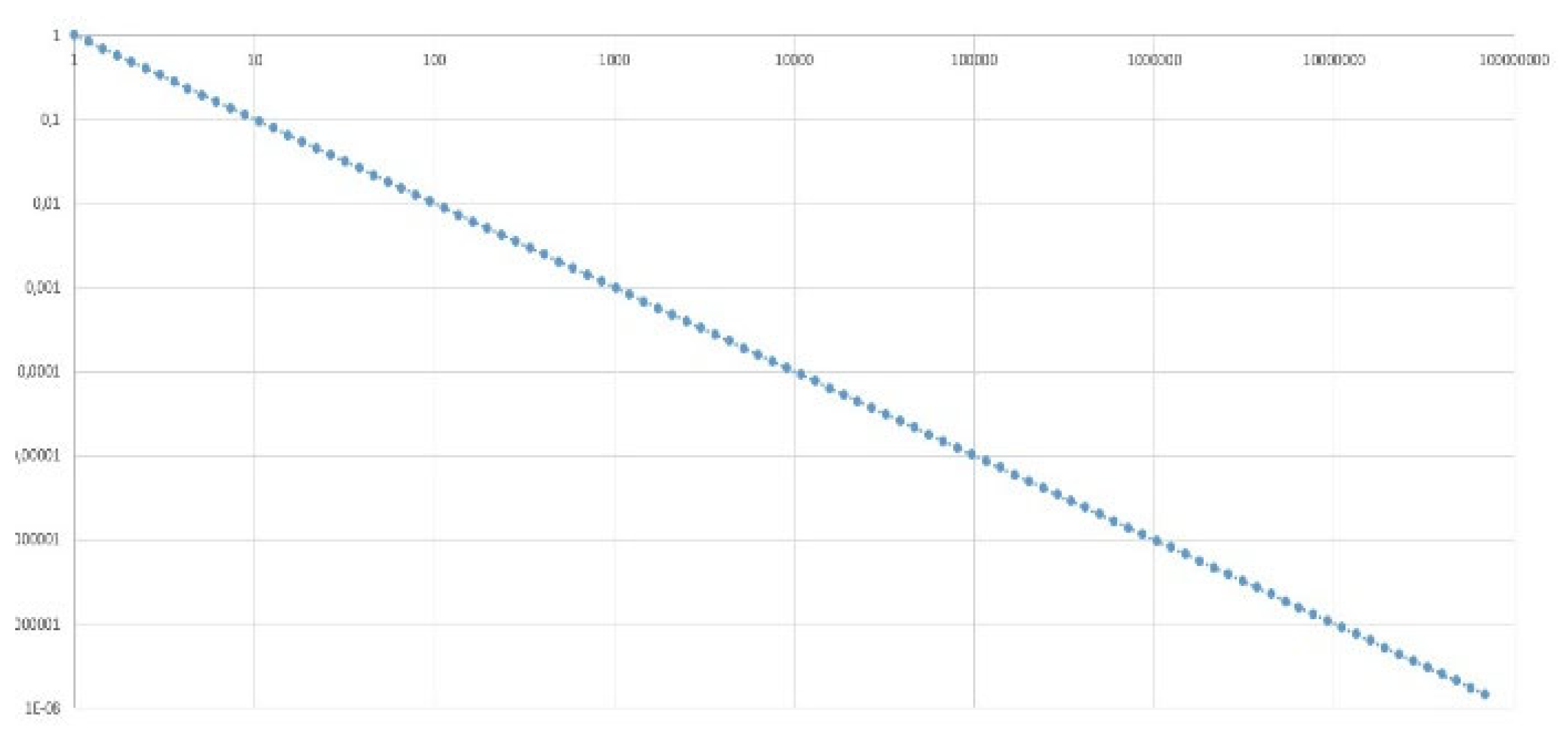
There is a remarkable feature in the graphs presented on a double logarithmic scale. As a rule, all such graphs can be described with a fairly good approximation by several straight line segments, especially if the connecting points of these straight lines are slightly smoothed. The fact is that the logarithm of the product of functions is equal to the sum of the logarithms of these functions. Moreover, if one of the factors is two or more orders of magnitude larger than the other factors, then these factors actually do not affect the result. For example, if a function depends inversely on its argument, then on a double-logarithmic scale it represents a line with a negative slope.
Here and everywhere below, the decimal logarithm is used. The first term gives only a shift of the graph up or down, the second term describes a line with a slope
, where
it means a 10-fold change in the value displayed on the graph. Such a function increases indefinitely as
. When
this value (5) tends to infinity. Accordingly, the logarithm of a quantity
tends to minus infinity, and the logarithm of the inverse quantity, that is, the logarithm of a quantity
taken with a negative sign, tends to infinity with a plus sign.
Figure 2 shows the characteristic form of dependence of type (5) on a double logarithmic scale.
If in some area the function weakly depends on the argument, it is displayed by a line parallel to the x-axis:
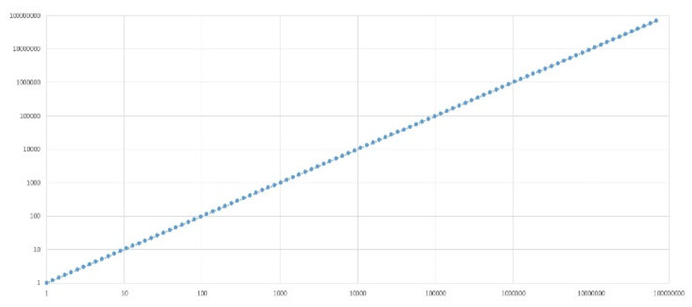
If a function in some area changes almost linearly with increasing argument, then its graph is a straight line with a slope
:
When
the logarithm of this quantity tends to infinity, as does the logarithm of this quantity:
Figure 3 shows the characteristic form of a dependence of type (8) on a double logarithmic scale.
If quantity (3) includes factors that depend on and on the reciprocal quantity , then they are not simply multiplied with compensation for each other, but have different effects in different parts of this function.
Therefore, just the hypothesis that the function
depends on the argument
according to a power law, where there are terms with different degrees, both positive and negative, allows us to quite accurately describe the qualitative appearance of this graph. For example, consider a function like this:
Let’s put this expression in logarithmic form and get:
Here
,
. If the equation
= 0 has real roots—
T1 and—
T2, then function (11) can be represented in the following form:
Let us assume for definiteness that
. Then we divide the entire x-axis into three intervals:
On the first interval
,
, therefore
This is the equation of the slanted line (5) with a negative slope.
On the second interval
,
, therefore
This is equation (7) of a line parallel to the x-axis with zero slope.
On the third interval
,
, therefore
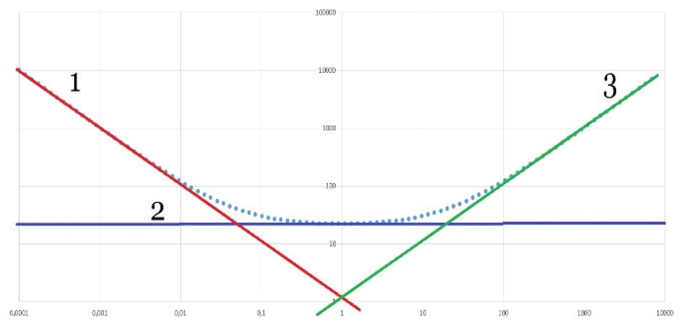
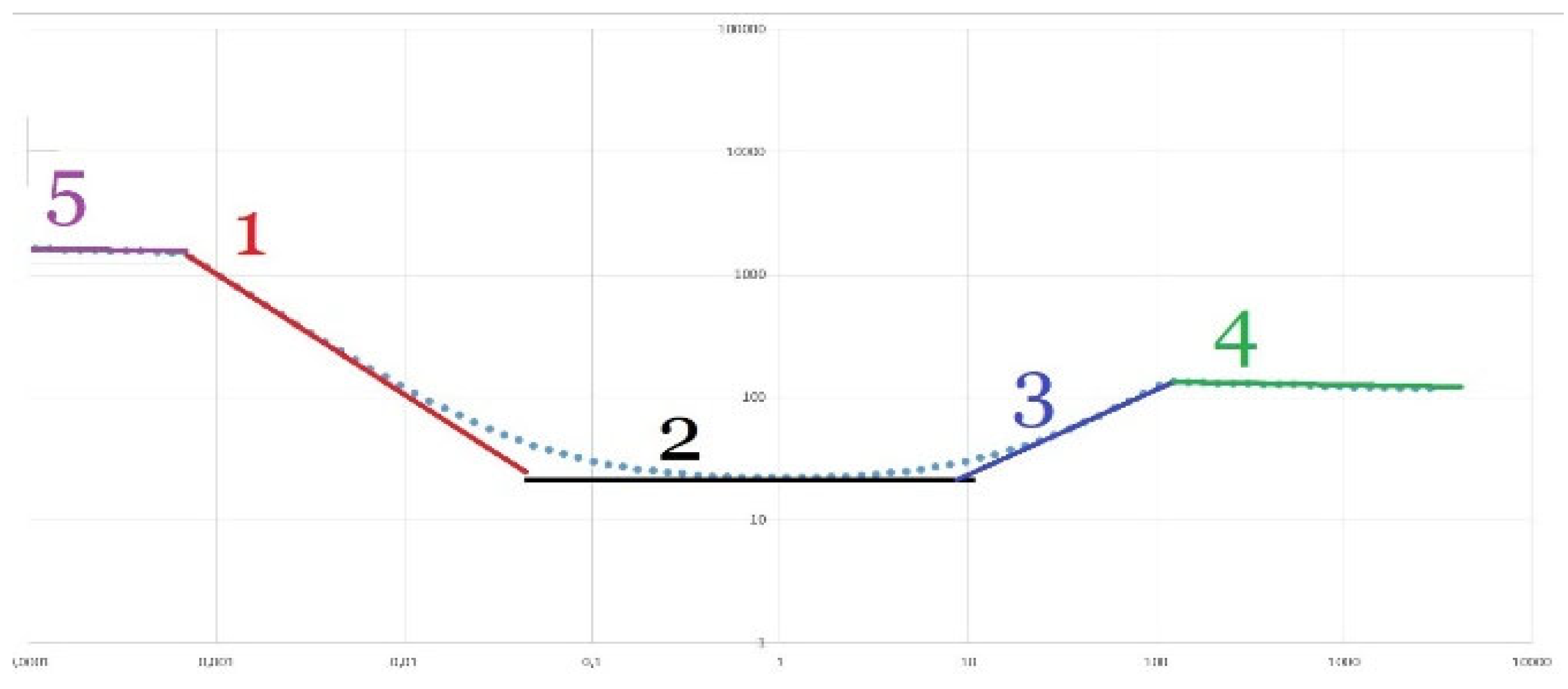
This is equation (8) of an inclined line with a positive slope. Thus, a function of the form (10) in the general case has the following form, as
Figure 4 shows: on the left side it asymptotically approaches the inclined line of the form (14), on the right side it approaches the asymptotic line of the form (16), and the section of the form (15) in the middle part may exist or be completely absent. This section exists if the graphs according to equations (14) and (16) intersect lower than the graph according to equation (15). If they intersect higher, then the section according to equation (15) is absent, the branch with a negative slope smoothly turns into a branch with a positive slope, practically without a section with zero slope.
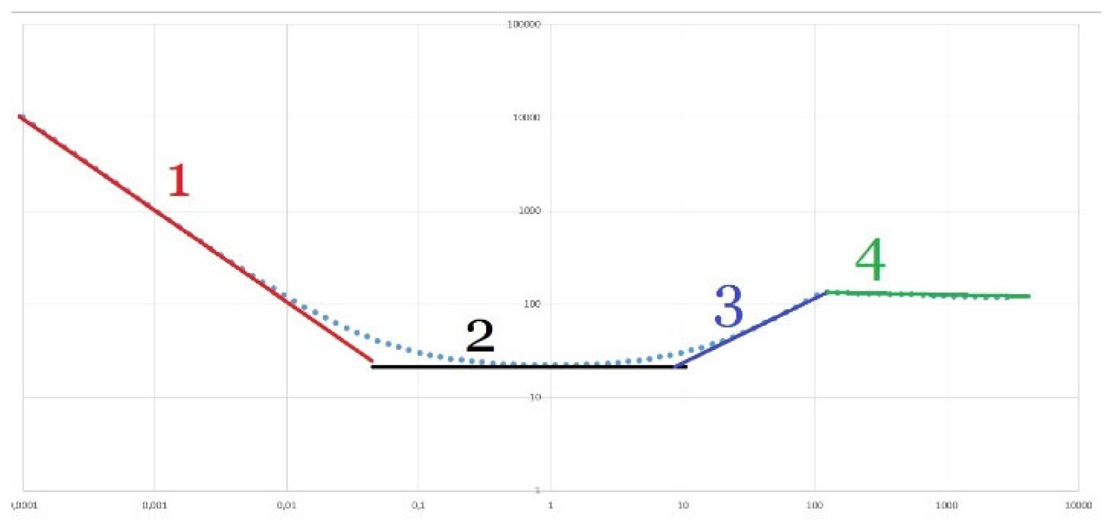
If we talk about possible types of an arbitrary function on a logarithmic scale, then we can consider asymptotes with a different slope, in addition to the considered asymptotes with a slope of -1, 0 and +1. In particular, if there are terms containing , then an asymptote with a slope will appear on the rightmost side of the graph. If there is a term containing , then an asymptote with a slope will appear on the left side of the graph The term with a multiplier will give the conjugate section between the asymptotes with a slope and with a zero slope, and the slope of this section will be equal to .
The term with the multiplier will give the conjugating section between the asymptotes with zero slope and with slope and, and the slope of this section will be equal to . Both of these sections may not appear if the corresponding graphs are completely below the other fragments. So, the assumptions discussed above about the form of this function were made solely on the assumption that the function depends on the argument according to a power law; no additional theoretical or experimental information was used for these conclusions.
we put in the denominator of function (12) , then the left side of the graph will not increase indefinitely, but only to the value . If we introduce another factor of this type into the denominator of relation (12) , provided then the right side of the branch will not increase indefinitely, but only up to a certain value that can be calculated from the given relations, after which the graph will again run parallel to the abscissa axis, and if add another such factor to the denominator under the same conditions, then the right side of this graph after a certain value will begin to decrease with the slope , gradually tending to the value minus infinity on a logarithmic scale, that is, to the zero value.
Figure 5.
Graph of a function of type (10) on a double logarithmic scale if the asymptote according to relation (15) passes below the largest value of the other two asymptotes: 1—asymptote according to relation (14), 2—asymptote according to relation (16).
Figure 5.
Graph of a function of type (10) on a double logarithmic scale if the asymptote according to relation (15) passes below the largest value of the other two asymptotes: 1—asymptote according to relation (14), 2—asymptote according to relation (16).
Rütmann, a classic in this field, reports: “For a particular generator
represents the sum of two or three terms; thus, atomic standards in a cesium beam are often satisfactorily modeled using the expression
Moreover, the values
and
can be determined from measurement data
if
measured within a sufficiently wide range” [
2].
The indexing of the coefficients is surprising. Why the coefficient for the free term has the index “
”, and the coefficient for
the power “
” has the index “0”, this is not clear, it should be the other way around. In addition, the meaning of introducing a logarithm with a coefficient of “2” is not clear; it is enough to simply give the coefficient
, because its numerical value is not defined in any way. There is also no need to enter a two in the denominator in the first term; it can be absorbed by the coefficient. In the terms used, it would be more logical to give the following model:
This model coincides in the case of changing letter designations with model (10), provided that the last term in relation (10) takes a zero value due to the zero coefficient.
. The graph of such a function corresponds to a line that approximately coincides with the larger of the two asymptotes in
Figure 4, with the asymptotes numbered 1 and 2. Practice has repeatedly shown that the model given by relation (10) is more often obtained as a result of experimental studies of the stability of atomic and laser frequency standards, which can be confirmed by many bibliographic references.
Actually, increases with growth or does not increase is an extremely important question, it is fundamental.
The question of whether the Allan parameter function is parallel to the abscissa axis, or whether it has a positive or negative slope is the question of fundamental importance. If the slope is zero or negative, then the generator or laser under study has no frequency drift, so it can be considered as a potential prototype of a future frequency standard. If the slope is positive, then the generator (laser) under study cannot even pretend to be considered in this role. Thus, a zero or negative slope of the Allan parameter graph in the region of large “tau” is a necessary but not sufficient requirement for any prototype of a frequency standard. Thus, the analysis of this graph in this area is of fundamental importance. At the same time, we have come across publications where the specified graph is presented as a characteristic of such a generator, and the author does not pay attention to this discrepancy. An example is the article [
35]. This article presents a graph of the Allan function in which the right branch is reliably directed upward, as is the left branch. This graph is interpreted by the authors as evidence of the high stability of the created frequency standard prototype, and the most important characteristic of this prototype is the point of the minimum value of this function, which we dispute, arguing that it is much more important how this function changes at
.
The left branch of the graph, caused by a component inversely proportional to
, is obtained in absolutely all experimental studies. This is explained, first of all, by an increase in the error in frequency measurement using the counting method. It will be shown below that this error can be reduced due to a specially created measuring device, which proves the fact that the first term in relations (17) and (10) is not determined by the properties of the frequency generator (laser, quartz oscillator, laser frequency standard, or atomic frequency standard) namely, the frequency measurement method. If this term were inherent in the generator itself, and not in the measurement method, then replacing the measuring device would in no case reduce the coefficient of this term. Since the decrease in this coefficient has been experimentally proven, then the true dependence of the value
in this first interval
is less than this term, and the graph of this function on a double logarithmic scale lies below the graph of function (14). There is every reason to believe that the true value of this quantity
not only does not tend to infinity, but even tends to zero, which is expressed by the simple statement: “The frequency of any source of oscillation cannot change abruptly instantly,” that is, in zero time the change in this frequency equals zero. An infinite increase in noise in the region of zero frequencies cannot be related to the noise of any physically realizable generator, since the spectrum of frequency noise is always limited in frequency, a function with a limited frequency spectrum cannot undergo jumps in zero time, a finite spectrum means the differentiability of this function. The term “frequency” is correct only for a random narrow-band process, i.e., a process with a limited spectrum [
36], a limited spectrum means zero jumps in strictly zero time.
Regarding the right side of the graph of the function shown in
Figure 4, the following theses can be consistently put forward and proven, based on the assumption that the model of type (10) is incomplete.
In the first step, we will consider whether the actual value can in practice increase with growth according to a power law, which on a double logarithmic scale is represented by a linear increase in the graph, and if this is possible, then under what conditions.
Next, we will consider the assumption that, perhaps, this function not only does not increase indefinitely with growth, but also decreases in some way. We will also consider the conditions for fulfilling this assumption.
Finally, we will consider how legitimate it is to assume or even assert that the indicated function not only simply decreases with growth, but also tends to zero in the limit at.
First, let’s make two disclaimers.
Firstly, the measurement error of function (4) at different value intervals differs significantly, by several orders of magnitude. This means that the confidence interval for an experimentally obtained graph is not some band around the experimentally obtained values, but can have a more complex form, in particular, expand, for example, proportionally or inversely proportional to the value .
Secondly, we agree that the results of measuring the specified function (4) not only may differ from its true value, but also almost certainly differ from the true value, which does not make the measurement of this dependence meaningless. If the error is insignificant compared to the actual value, it can be neglected. If the error significantly exceeds the measured value itself, then such a measurement should not be trusted. The problem here is that the measured quantity itself is, as a rule, extremely small, so the value of the quantity itself and the error in its measurement may differ by several orders of magnitude in some value intervals. . For example, to increase the measurement error inversely proportional to the left side of the graph, it is quite natural and understandable, while an increase in frequency noise itself according to this law contradicts the physical nature of frequency noise.
Thirdly, we note that the method of measuring quantity (4) under certain conditions can not only overestimate the result, but also underestimate it, that is, the obtained values of quantity (4) at some value intervals may be less than the actual values.
Ryutman further writes: “Linear frequency drift leads to a dependence of the form τ
+1 for the square root of the two-sample variance. This dependence is observed at large values of τ, when a linear frequency drift cannot be excluded before statistical processing” [
2].
This is indeed true: linear growth of a function
is possible only if the value itself
linearly depends on
. Indeed, let, for example, this function have a linear form:
Here
is random noise with zero mean:
When averaging over a large time τ based on (19), the third term in (18) can be neglected, so we can write that
Substituting this value from (21) into (3), we get:
So, indeed, the dependence of the Allan function in any range proportionally indicates linear regression. Precisely linear, and not just some arbitrary frequency drift. That is, the generated frequency has an unambiguous trend: the more time passes from the start of measurements, the further the frequency goes from the initial value, and this happens continuously, linearly, that is, at some constant speed and only in one direction; the frequency does not return back, it never receives increments in the opposite direction, with the exception of short deviations in both directions with zero average, which is indicated by the third term in relation (18).
Now it makes sense to ask the question: for what reasons can a generator that generates a frequency, the value of which continuously changes in one direction at a constant speed, be considered stable?
Suppose that the frequency first changes at one rate and then at another. In this case, it is possible to determine the average speed over the entire interval and assert that this is precisely the component of linear drift.
Let us now assume that the frequency changes first in one direction and then in the opposite direction, for example, first it increases, then it decreases. Then the average global drift is equal to the average speed over the entire interval, which, taking into account the sign, will be less than each of these components. Consequently, in the first part of this interval, when the frequency, for example, only increased, the drift value will be greater than the average drift over the entire global interval. Also the average drift in the second section of the interval, when the frequency decreased. Therefore, in this case, linear drift will not occur, since the drift speed over a larger time interval will be less than over a smaller time interval. Therefore, there will be no linear relationship in this case.
Now let’s discuss whether in some physical installation, in a real physical generator, the frequency can change in one and only one direction at a constant speed for an unlimited time?
Any generator can generate frequency only within a limited frequency range. In addition, for almost any physically realizable generator, even without the use of stabilization methods, the frequency , which varies in a certain range, can take on a certain value at each moment of time, and this is a random variable with a distribution, as a rule, according to the normal distribution law. This hypothesis is incompatible with the hypothesis of linear frequency drift with some fixed average rate unlimited in time according to relation (18). Thus, there must necessarily be a turning point on the graph , after which the growth of this function stops, and then, at a minimum, it does not increase.
If the graph of changes in frequency over time has several periods of oscillations, regardless of their shape, then averaging over intervals in which several periods fit gives, of course, a significantly smaller difference between the two results of subsequent averaged measurements than averaging over intervals equal to a quarter of the period of such hesitation. Consequently, for such a dependence of frequency on time, the value of the Allan function decreases with increasing .
So, if there is a rise in this function with increasing τ, therefore, there is a continuous linear drift of the generated frequency. This drift must be eliminated.
In addition, if the authors of the study present an experimental graph of a function on a double logarithmic scale and the graph shows the growth of this function with increasing , this indicates that the information provided is not enough: it should be indicated from what value the growth of this function, at a minimum, stops, and in a good way the frequency should be indicated, starting from which this function then decreases.
However, the continuous increase in the Allan function (4) with increasing is not necessarily explained only by linear regression of
. It can also be fully assumed that the error in determining this function by experimental methods increases due to some reasons, one of which is, for example, non-zero dead time in the experimental measurement of the average frequency over an interval, another is incorrect averaging of the frequency over an interval as a consequence of the presence of dead time, the third the reason may be insufficient statistics for the graph points in this range of values.
.
Figure 6 shows the graph of the function
as it should be on a double logarithmic scale for any real oscillator, since the frequency
varies only over a limited range of values, so it cannot increase or decrease linearly over an infinite time interval. Eventually, the frequency drift should weaken and even change sign.
If the frequency standard is characterized by a linear regression of frequency, then either the limits of permissible changes in this frequency or the time frame for the specified regression should be estimated and specified. Otherwise, the frequency, changing continuously at a constant speed in one direction, can reach any value, which, of course, does not happen in any real generator. But if physical boundaries for frequency values or time frames for regression are indicated, this indicates that in fact there is no linear regression, but only a fragment of it. Thus, indicating that a function grows with growth is an insufficient description of the properties of this frequency standard: either it is so bad that this function actually grows to indefinitely large values, or this frequency standard was not properly certified, and the measurements were obtained with such large errors in this part of the graph, that the actually stopped growth of this function was not detected experimentally due to the large error values in this range of values , which is of particular interest to any user. Indeed, the behavior of the function with growth , although it does not provide specific information about the significance of the instability and irreproducibility of the value , is related to these values more closely than the lowest point on this graph.
Based on the experience of studying frequency noise of laser and atomic frequency standards and developing equipment for measuring them, as well as based on the above reasoning and calculations, the following can be stated.
Conclusion 1. The rise of the experimentally obtained Allan function with increasing τ is not always associated with linear regression, but can be generated by measurement errors, including insufficient statistics for large time intervals τ, or incorrect sampling, or periodic frequency modulation of the generators under study at some frequencies and the lack of experimentally obtained points of this graph at the highest values of τ. In combination, these two factors can give a significant measurement error, which can be taken as a true increase in this function at .
Let us also discuss the behavior of the function as τ decreases.
Frequency noise is a random process with a limited spectrum. An unlimited increase in the dispersion of this noise with increasing frequency would indicate the possibility of an infinite increase in frequency over an infinitesimal time interval, which contradicts the principle of physical realizability. Even if such a generator existed, it would not be possible to accurately transmit its frequency noise to a measuring device, because the frequency of, for example, a laser frequency standard is measured using a conversion path that contains a photodetector and bandpass amplifiers, which also have a limited bandwidth. The idea that a physically realized process can be characterized by an increase in noise in the region of infinite frequencies to infinity is clearly erroneous.
This conclusion can be justified by the following reasoning. If we imagine light as a stream of photons, then the shorter the time interval considered, the fewer photons are emitted by this light. Theoretically, there is such a small value of τ that on average only one photon is emitted. Each photon has a radiation frequency described by Planck’s relation and, presumably, the photon does not lose energy, since it is considered as an elementary particle. Thus, the radiation spectrum can be represented as a superposition of a limited number of quasi-harmonic signals per unit time, something like a sum of damped oscillations, each of which has a constant carrier frequency. The spectrum of such a signal is, of course, limited, as shown in
Figure 7.
Conclusion 2. The increase in the resulting estimate of the Allan function with a decrease in τ is associated with the hardware error of the digital frequency meter. The true Allen function in the region is described by a descending asymptote towards , rather than an increasing asymptote. That is, the function, when moving along the graph to the left, does not increase, but, starting from a certain value, decreases down to zero, which corresponds to minus infinity on a double logarithmic scale. It should be understood that since the measurement error of the function estimate inevitably increases with decreasing τ, the experimentally presented graph will have the opposite trend, it will increase with decreasing , but this should not be attributed to the properties of the generator.
4. Methods for Experimental Measurement of the Allan Function
To measure the Allan function, it is necessary to obtain a sequence of average frequency values at closely adjacent time intervals of equal duration [
2]. The duration of each such interval must be strictly equal
. Traditionally, the average frequency over duration intervals
is measured by the counting method. Thus, a series of average readings is obtained over intervals of frequency values. Let us denote the duration of the shortest possible interval by
. In this case, we can denote a series of readings
we omit the averaging sign in the form of a bar over the value, which was used in relation (3), so as not to unnecessarily complicate the form of further relations for
.
From this sequence we can obtain a sequence of differences between two successive measurements, as shown in
Figure 8:
Next, to obtain one point of the desired function,
it is enough to find the root mean square value of sequence (25):
Also, from these values (24) you can calculate , where is any positive integer. Traditionally, in order to save computing resources, they were used only for values, for example, equal to some power of two. In this case, the resulting calculated points of the Allan function are distributed evenly on a double logarithmic scale with a distance between them equal to . However, this is not entirely reasonable. We propose to calculate and plot the Allan function for all positive integers , since technical means with the correct software can easily do this and even display the resulting graph in real time, and the advantage of this approach is that instead of individual points on the graph we get a line from many points. This line’s behavior in the area of low values differs sharply from the behavior in the area of medium values and from the behavior in the area of high values. The fact is that in the region of small values , as a rule, sufficient statistics to obtain a reliable result, statistically independent of random measurement deviations, are obtained quickly enough; this does not require long-term measurements. However, each subsequent value requires several times more experimental time to accumulate the same number of statistically significant measurement results. For example, if to obtain a result with sufficient accuracy for a certain value, measurements for a duration of 1 minute are sufficient, then it will take an hour, for a whole day it will be required, and for a continuous measurement over a whole year will be required. If the measurements are limited to only one day, in this case, the collected measurement results for large values of the time interval will be statistically insufficient, and therefore the result will be statistically unreliable. This fact should be displayed on the graph in the form of confidence interval marks or in the form of measurement error marks on either side of the experimentally obtained points. But if we count the values for all positive integers , then we get fluctuations in the experimental graph due to different values for and for , as well as for and so on. If , then , therefore there should be no sharp fluctuations in such a schedule. Therefore, these fluctuations demonstrate statistical measurement error. Indeed, as the number of measurements increases, the updated graphs of the function tend to reduce deviations from the average in a larger and larger range of values ; this compression of the oscillating line occurs the more strongly, the further to the left the corresponding section of the graph is located, since for the leftmost values of the argument more values can be calculated, made up of primary measurements. Thus, the amplitude of fluctuations in the experimental graph demonstrates the error of this experimental result in a given range of arguments; the smaller the amplitude of the deviations, the smaller the error of this estimate. The operator managing the measurement experiment can decide in real time whether the accumulation of measurement results should continue, or whether sufficient statistics have already been accumulated to calculate the values of the Allan function in the required range of time intervals with an error not exceeding a specified maximum value.
This approach to processing the results also solves the problem that Rutman expressed with concern, namely, the problem of the influence of periodic noise on the result of estimating the Allan function. If the period of this interference turns out to be a multiple of some specific value of the measurement interval, then this interference can give an unreasonably larger increment to the Allan function, both in the positive direction and in the negative direction, depending on the phase relationships. When using the proposed method, such a deviation will occur only at some points, and neighboring points will not be characterized by this deviation, since the phase relationships there are different and the multiplicity will be violated. Thus, sharp awl-shaped increases or decreases in the Allan function at some individual points will be easily identified, and they will be recognized precisely as the result of the presence of a periodic component in the frequency change function, and not as a change in the Allan function near the corresponding value of the argument. Thus, calculating the values of the Allan function for all values eliminates the need to invent and implement a method for determining the error in the experimental assessment of this function; such an assessment is obtained automatically and is clearly displayed on the graph in the form of deviations from the trend.
In the literature, it is often erroneously stated that all successively changing intervals occur, with a slope inversely proportional to
(i.e.,
), inversely proportional to the root of
(i.e.,
), the section independent of
(i.e.,
), the section, proportional to the root of
(i.e.,
) and proportional to
(i.e.,
). In fact, the two intermediate sections are simply the result of conjugating sections with slopes proportional
to an integer power (minus one, zero and one), as shown in
Figure 4. The statement about the existence of extended sections with slopes
and
is, apparently, the results of incompetent or dishonest research, such sections are taken to be ordinary conjugating sections; if the length of such sections does not exceed one decade, there is no reason to talk about the root dependence of the Allan function on
.
In order to understand how the Allan function can and should change depending on noise and on the parameter , one should give an interpretation of this relationship, and one can also use analysis using both an analytical method and a numerical modeling method. In essence, relation (4) describes the standard deviation of two subsequent measurements of the average frequency at two subsequent time intervals of duration . This understanding is sufficient to make the prediction that if the function increases linearly, then function (4) depends linearly, as shown by relation (23). Accordingly, a proportional dependence can occur if there is a constant frequency drift with a speed proportional to .
5. Simulation Research
Almost any noise-like function that does not change monotonically is characterized by a limited increase in its Allan function; this characteristic necessarily, after reaching a certain value, then begins to fall with growth . If the indicated graph continues to grow, this may be due to one of the following reasons: a) an increase in the measurement error in this area; b) insufficient range of consideration of the schedule; c) incorrect operation of the measuring device or incorrect processing of measurement results; d) an extremely low-quality generator that cannot in any way claim to be a frequency standard.
Simulations in the
VisSim software [
37] verified some theoretical assumptions that only a function that changes monotonically in one direction, for example, linear drift, can be characterized by a graph of the Allan function, which increases with increasing
. It has been experimentally demonstrated that all other types of noise result in a decrease in exponent (4) with increasing
.
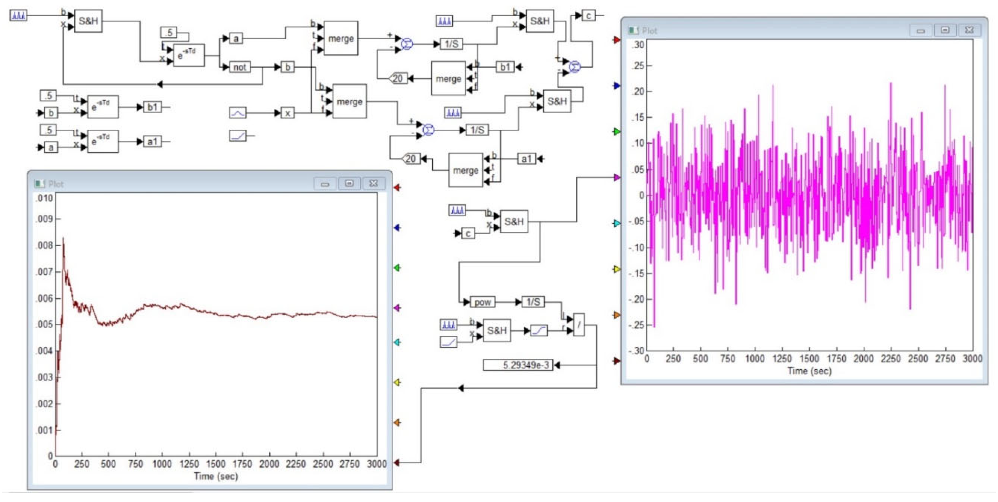
Figure 9 shows a project in the
VisSim program for automatically calculating the Allan function for a signal of any shape, including the signal from the output of a noise generator. In this project, to average a signal, it is used to integrate it over a given period of time and then divide the result by the duration of the segment. Integrators are denoted by blocks marked with the symbol of integration in the domain of Laplace transforms, that is, the symbol
. The value is stored using a sample-storage device, indicated in the diagram by a block with symbols
. Signal switches are indicated by the symbols
, and the project also contains summing devices, indicated by circles with the symbol
, squaring blocks, marked by the symbols
, a division block, indicated by the symbol “/”, as well as scale factor blocks with the coefficient value indicated inside the pentagonal symbol, as well There are signal delay devices, that is, pure delay links, which are indicated by a symbol
and bus marks, in the form of rectangles with a mark symbol in the form of a Latin letter with a number. All buses with the same marks are considered connected to each other. The signal under study is shown on the right side of the graph, and the result of calculating the Allan function is shown on the bottom left. It can be seen that while the number of measurements is not enough, this function undergoes changes, but then with an increase in the number of accumulated samples involved in averaging, the graph converges to its final value, the right side of this graph undergoes very insignificant deviations from the established value.
The simulation was carried out using signals of various shapes, including deterministic and stochastic signals, as well as their sums. For random and periodic signals, the Allan
function decreases, as expected, as. In the case of Gaussian, binary and homogeneous noise, the value of the Allan function begins to decrease sharply after the value
begins to exceed a quarter of the most characteristic oscillation period; if we are talking about a random signal, then in this case one should keep in mind the mathematical expectation of the oscillation period of this signal. The calculation error can reach 50% in the case when the measuring interval is no more than
. When the simulation time reaches the value,
the error in determining the Allan function does not exceed
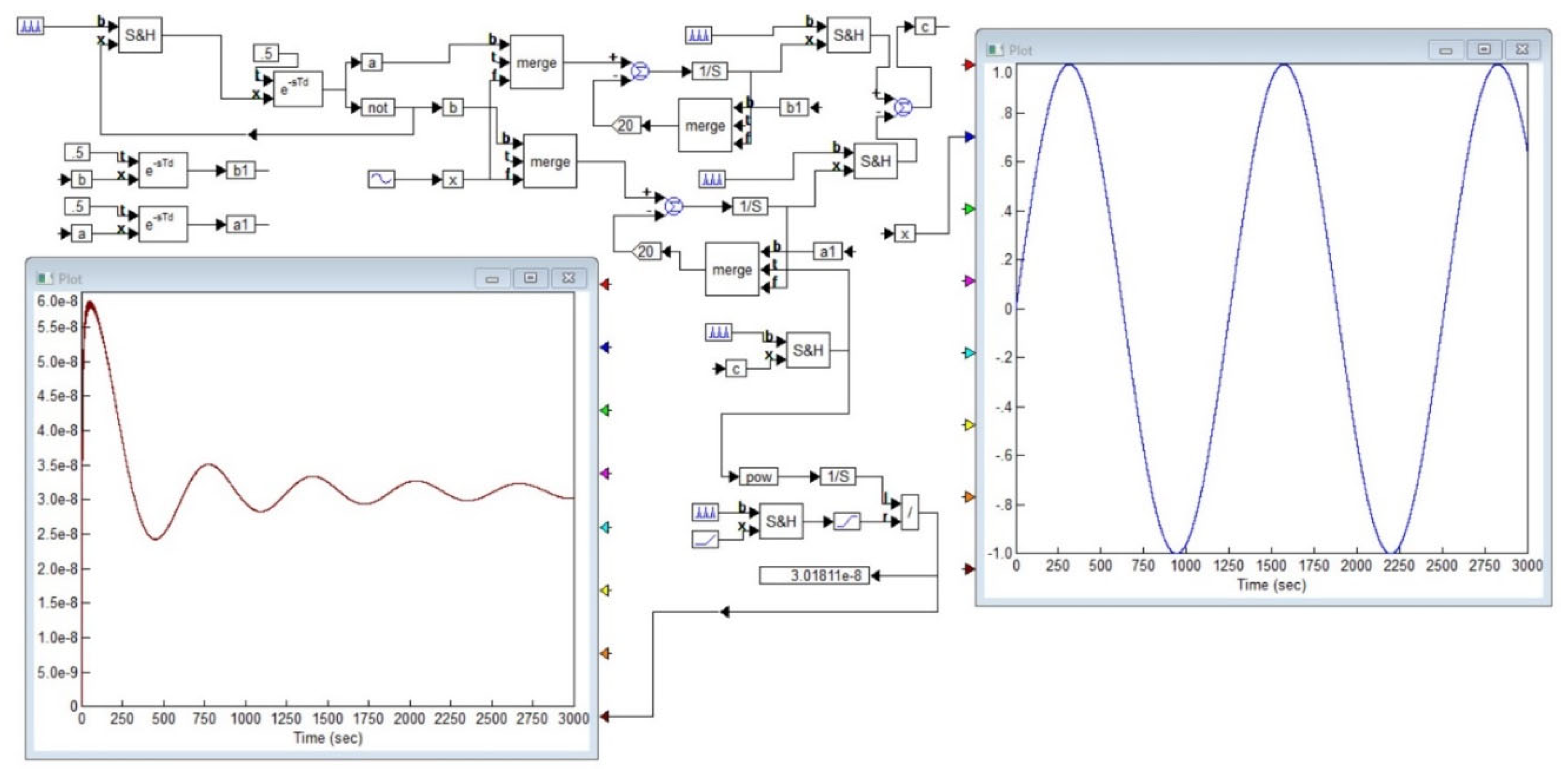
. As an example,
Figure 10 shows what the Allan function is for a harmonic signal. The value turns out to be several orders of magnitude less than the amplitude of a periodically or chaotically changing function; this applies to a value changing according to a harmonic law, and a function in the form of rectangular or sawtooth pulses, and to noise: Gaussian, binary, homogeneous. With an oscillation amplitude of one conventional unit, the value of the Allan function even
decreases over time to a value of the order of
. As it increases,
the Allan function decreases steadily for both regular periodic functions and noise-like functions.
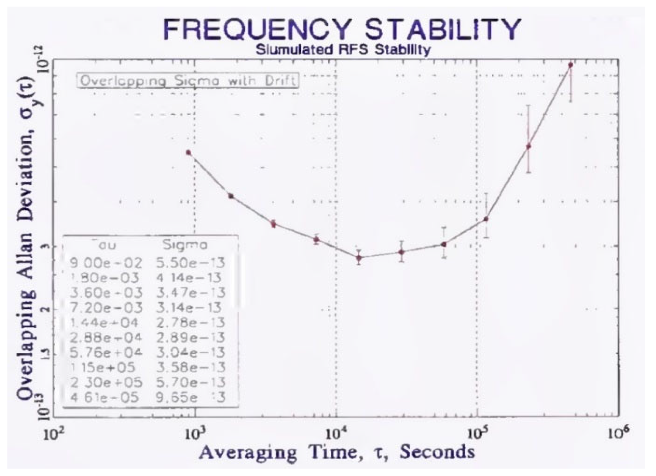
Let us discuss the statements given in various literature. For example, in [
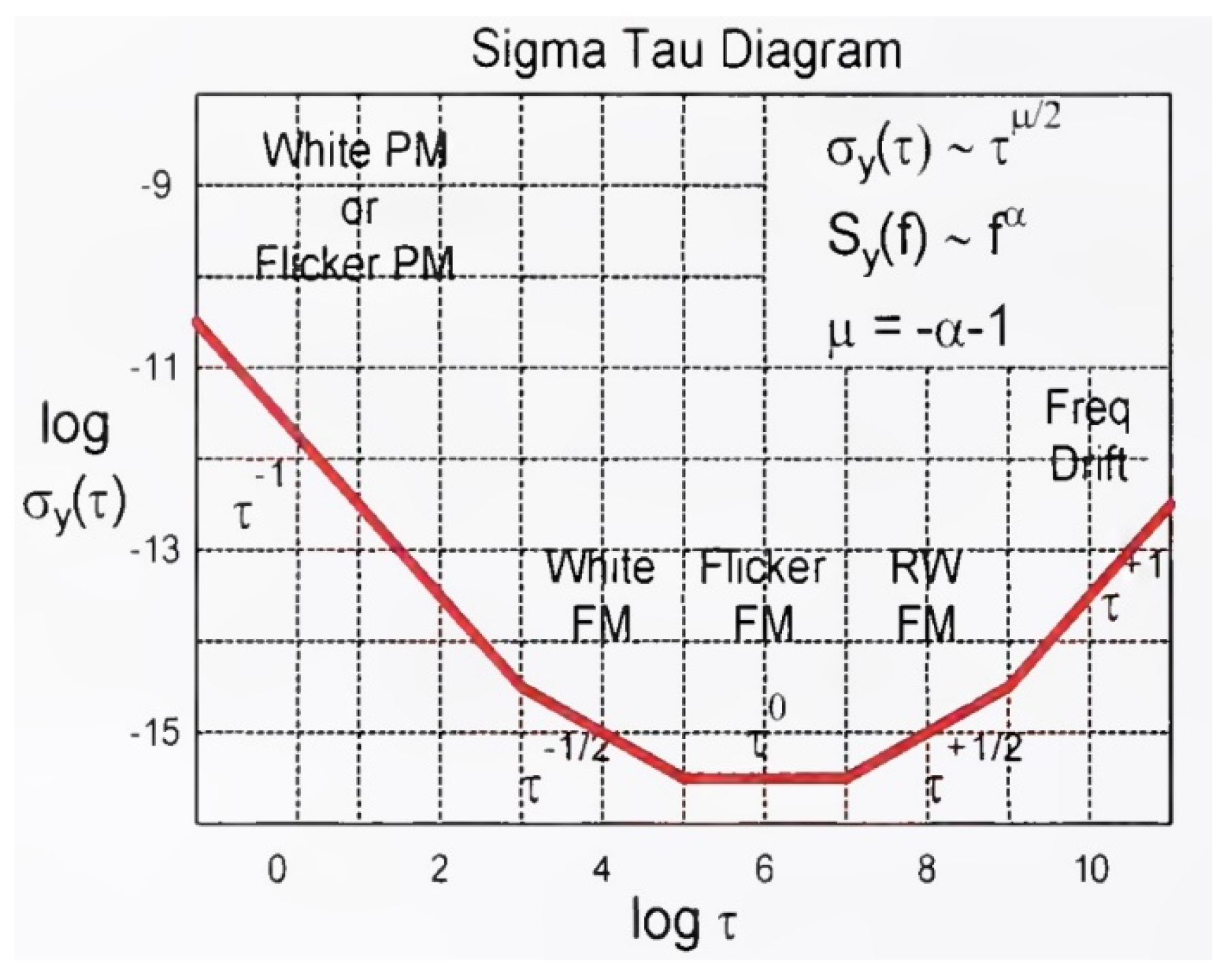
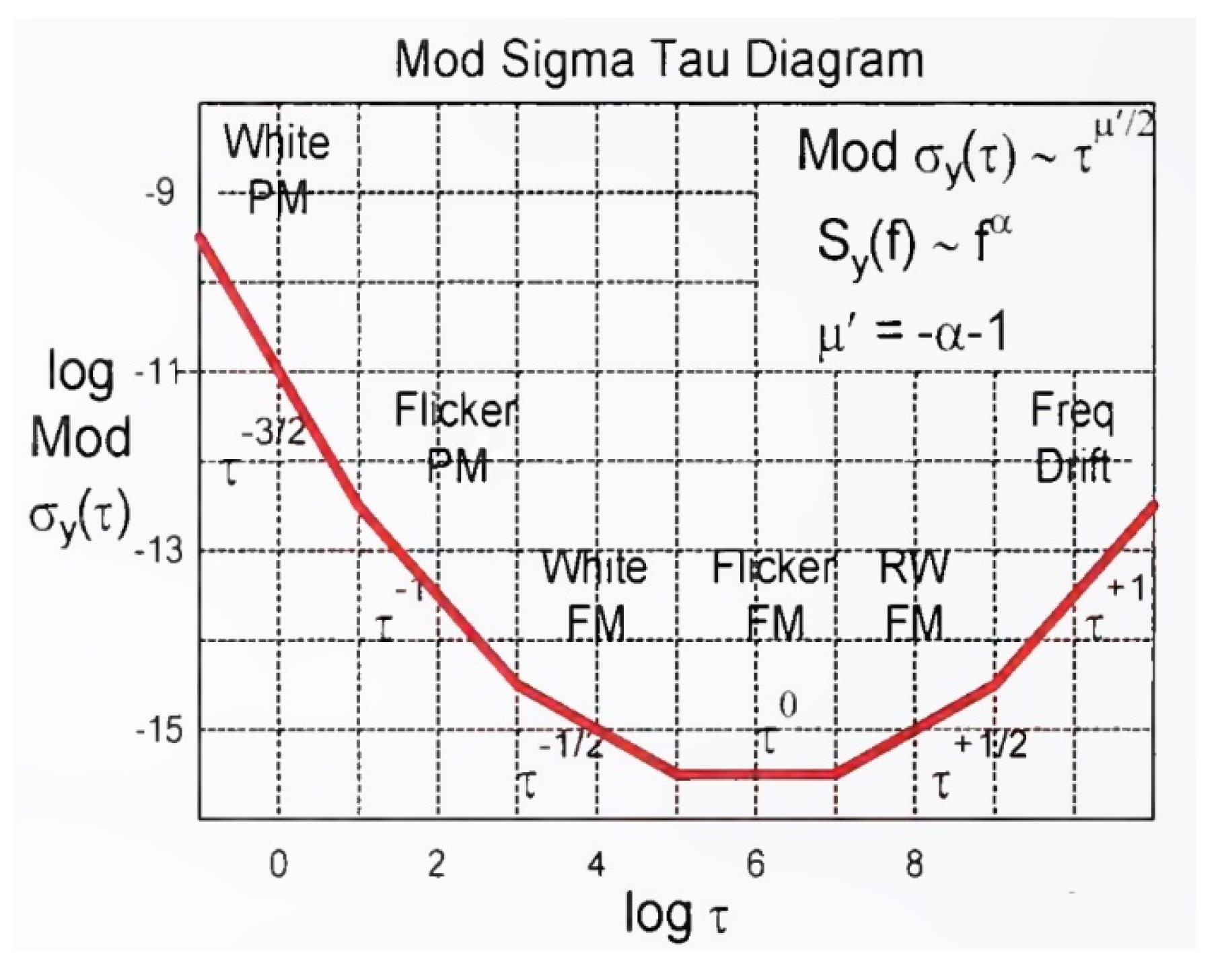
3] it is stated that the characteristic form of the Allan function looks as shown in
Figure 11 and
Figure 12. These options are erroneous both with respect to the left asymptote, and with respect to the right asymptote, and with respect to the conjugate sections, since with a length of no more than two decades, similar sections are simply a consequence of the conjugation of sections with integer slopes of the first and zero orders. The growth of this value on the left, especially in proportion to
, is an error; here, the error in measuring the average frequency by some specific instrument over extremely short time intervals is mistakenly taken for the statistical properties of the original signal under study.
Let’s look at the right side of the graphs. In [
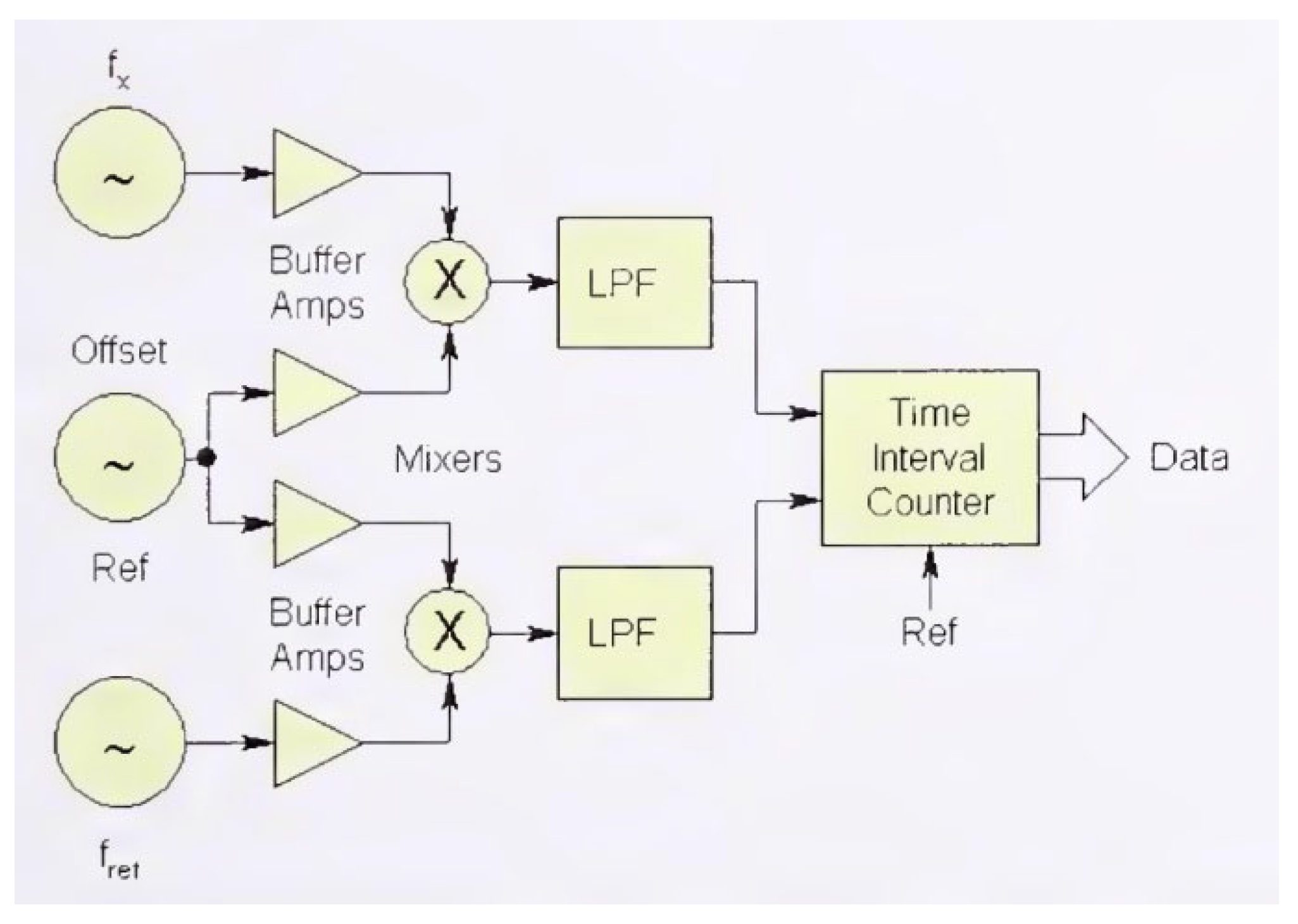
3], in particular, one of the methods for measuring the Allan function is given according to the scheme shown in
Figure 13. This method cannot reliably measure the properties of frequency noise in the high-frequency region, that is, in the region
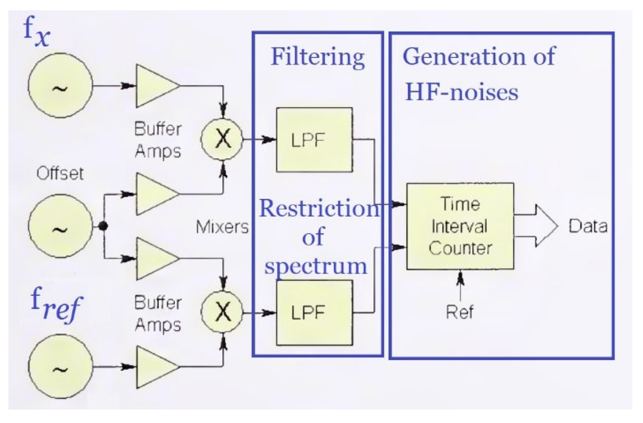
. For clarity, in
Figure 14 we highlight two blocks. The first block is a low-pass filter block. It cuts off high frequencies from the spectrum of the signal being studied. Therefore, measuring the high-frequency noise components of the remaining signal makes no sense. The next block after this block is the block of time interval counters. It is used to measure the average frequency at short intervals. The characteristic error of such counters depends on the averaging time
in inverse proportion, with a coefficient of the order of 0.5. Without special measures, consisting of creating and using an additional channel to refine the measurement result by 1000 times, any counting type meter is characterized by an error of 0.5 Hz per interval
and, accordingly, an error of 5 Hz per interval
, and so on.
In our series of publications [
36,
38,
39,
40,
41,
42], we described a proposed and repeatedly tested method and hardware-software device for reducing this error component by three orders of magnitude, that is, it is equal to approximately
. Comparison of the measurement results with this meter with meters without a corresponding reduction in this error component convincingly shows that the left branch in the graph of the Allan function is explained precisely by the error of the digital frequency meter using the counting method at small and ultra-small intervals. Our meter is characterized by an error of 0.0005 Hz on the interval
and, accordingly, an error of 0.5 Hz on the interval
.
In [
3] there are also examples of fairly correct measurement of the Allan function in the ultra-low frequency region, such as the graphs shown in
Figure 15 and
Figure 16. In
Figure 15, this function, starting from a value of about
, stops increasing. This indicates a correct measurement and a fairly stable frequency of the generator under study, that is, the demonstrated lower limit of stability at the level
is quite justified. It can be expected and stated that with growth
this value will most likely not be exceeded. The same cannot be said for
Figure 16. The right side of the graph is inclined upward, even taking into account the increase in the error of these points, a tendency for the value of the Allan function to increase appears. Therefore, achieving record low order values for this graph
in no way characterizes such a frequency standard as stable or accurate, since this function
not only reaches a larger value with growth,
but also continues to grow rapidly, which should not be the case in practice, and which causes large doubt the results of these studies if they are taken from a real experiment.
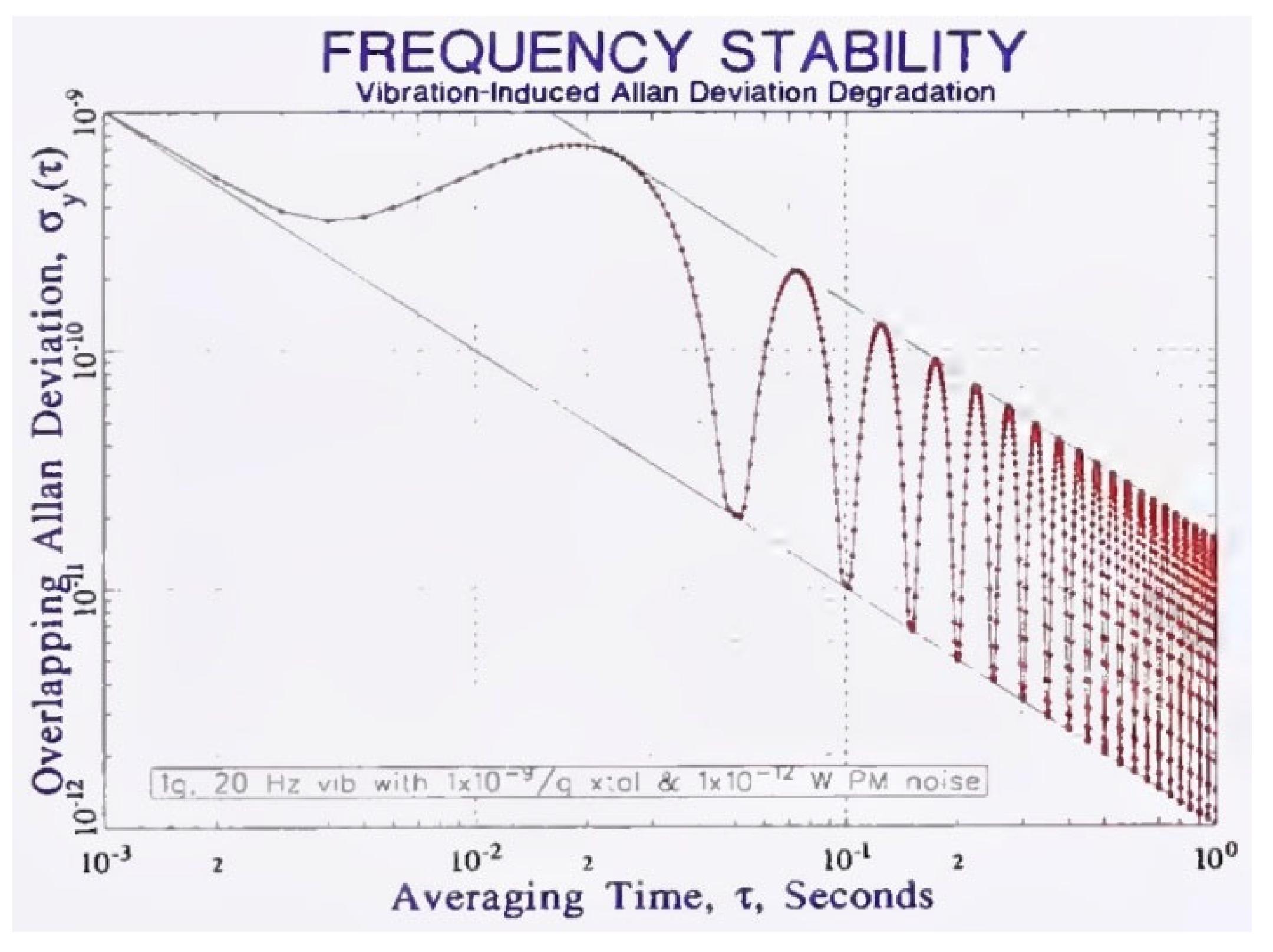
We will also consider how the Allan function should change in the presence of periodic deviation.
The work [
3] provides a graph, which is shown in
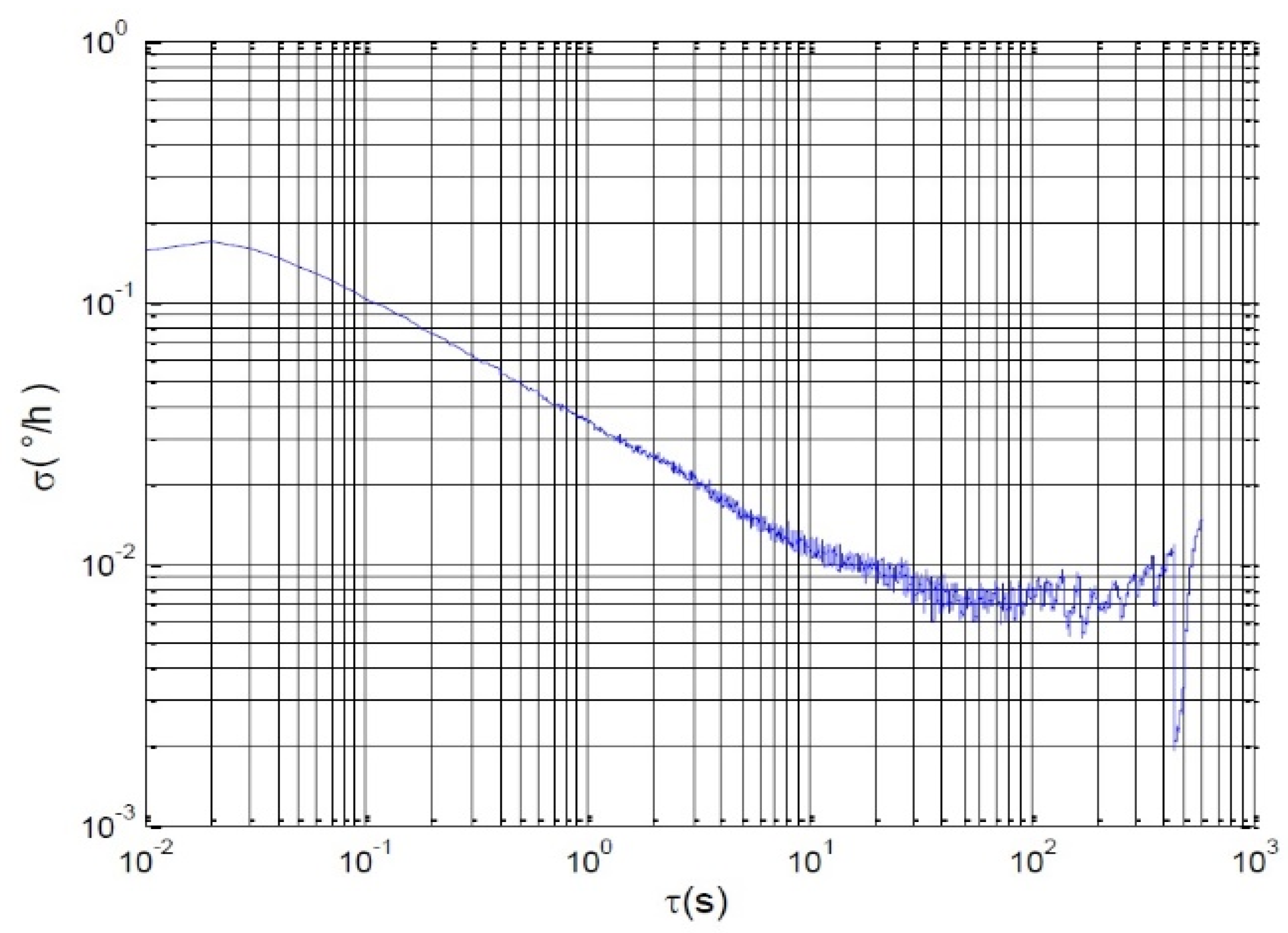
Figure 17. This graph shows deterministic fluctuations in the calculation result with a constant amplitude around a falling average and with an increasing frequency if evaluated on a logarithmic scale, which in fact reveals a constant frequency if The graph was on a linear scale. Natural noise cannot be described by such deterministic characteristics with clear periodicity. This result was obtained because signal generation and clock generation were used in processing from the same processor in the same computer. Therefore, the deviations turned out to be clearly synchronized with the measuring interval generator. Random deviations will not be so constantly synchronized, so there will be no such deterministic oscillations, they will be blurred, and a random process will result, as, for example, shown in
Figure 18 from publication [
4].
Discussion
In the literature there is a reference to the presence of dead time that occurs during measurements using the counting method. It is proposed to take this dead time into account and introduce some amendments. This is a completely unacceptable approach, since the problem of completely eliminating dead time has already been finally solved [
36,
38,
39,
40,
41,
42]. It is solved due to the fact that the counters that count counting pulses and count pulses of reference frequency never stop, but their readings are read on the fly, for which appropriate synchronization is applied. In this case, long counters are not required if reading occurs often enough, overflow and high-order bits are determined by software. Such counters never stop, therefore, there is no dead time in principle. Only with such counters can the Allan function in the region be measured with sufficient accuracy and reliability
, and only such counters can be used for the practical use of atomic and laser frequency standards as a time standard. If the counter has dead time, then the clock created on its basis will never be highly accurate; their relative error when measuring time intervals or when counting exact time will far exceed the relative error of the frequency standard itself used to synchronize measurements as a time standard. Therefore, it is high time to simply not raise the problem of dead time, keeping in mind that only frequency meters without dead time are used due to the specified technical solutions.
Based on the foregoing, it can be argued that some publications, such as article [
43], propose erroneous methods for measuring the Allan parameter, and also present erroneous results of such measurements. While there is confusion in this article between Allan variance
(quadratic function) and Allan variance
(rooted from the Allan variance), this work contains an erroneous notation
, which should already alert readers: such a relationship is impossible from the point of view of mathematics and is essentially erroneous; it could only be used with square brackets:
, only in this case the symbol of raising to the second degree would be appropriate. Also in the following relation
in the original the square at the end of the ratio is missing, which makes it incorrect.
But the main errors lie in the measurement technique. For example, article [
43] suggests using a closed-loop phase-locked loop system for more efficient use of the counting measurement method, as shown in
Figure 19. Any phase-locked loop system has a limited processing bandwidth, and only within this bandwidth does it transmit phase changes of the input signal to output, converting them into identical oscillator phase changes. Outside this band, such a system does not transmit any phase changes, and if there are phase deviations at the output outside this band, then they are generated by the instability of the applied oscillator without feedback, since outside this band the feedback has a gain coefficient less than unity and the effect of the feedback in this frequency range is negligible. For this reason, the graph of the typical dependence of the Allan function given in article [
43] is erroneous. On the graph, the ordinate axis indicates the Allan variation, that is, the Allan function or standard deviation, in which there cannot be a square. At the same time, the notation again uses an erroneous mathematical relationship containing an exponent of the second power, which cannot be there, as shown in
Figure 20. On a double logarithmic scale, it makes no sense to show any quadratic value, since the square is taken out from under the logarithm and gives a simple doubling scale:
. For this reason, quadratic functions are almost never constructed or studied in logarithmic axes; it makes no sense. The caption states that the graph shows the Allan deviation, not the variance. At the same time, a double slope is shown on the left and right edges, which indicates that a quadratic function was constructed, but the names on the axes cast doubt on this. In addition, the article uses strange terms, such as, for example, “absolute phase of the resonator,” without any explanation.
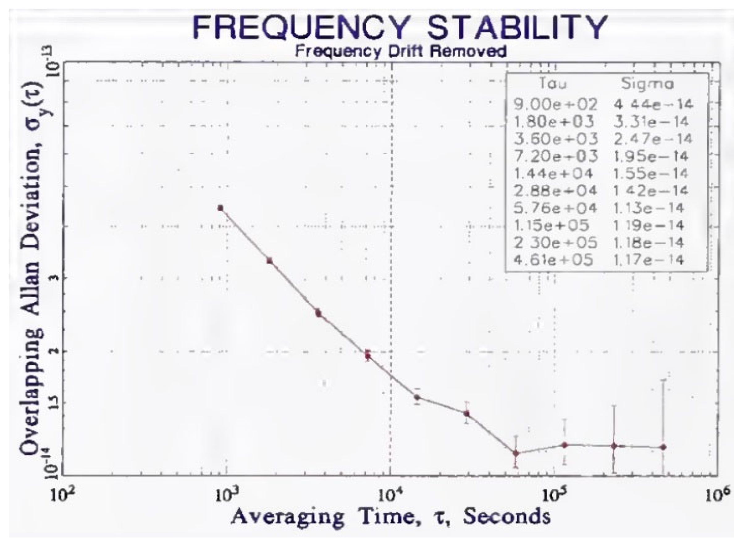
As can be easily seen, in
Figure 18, taken from the publication [
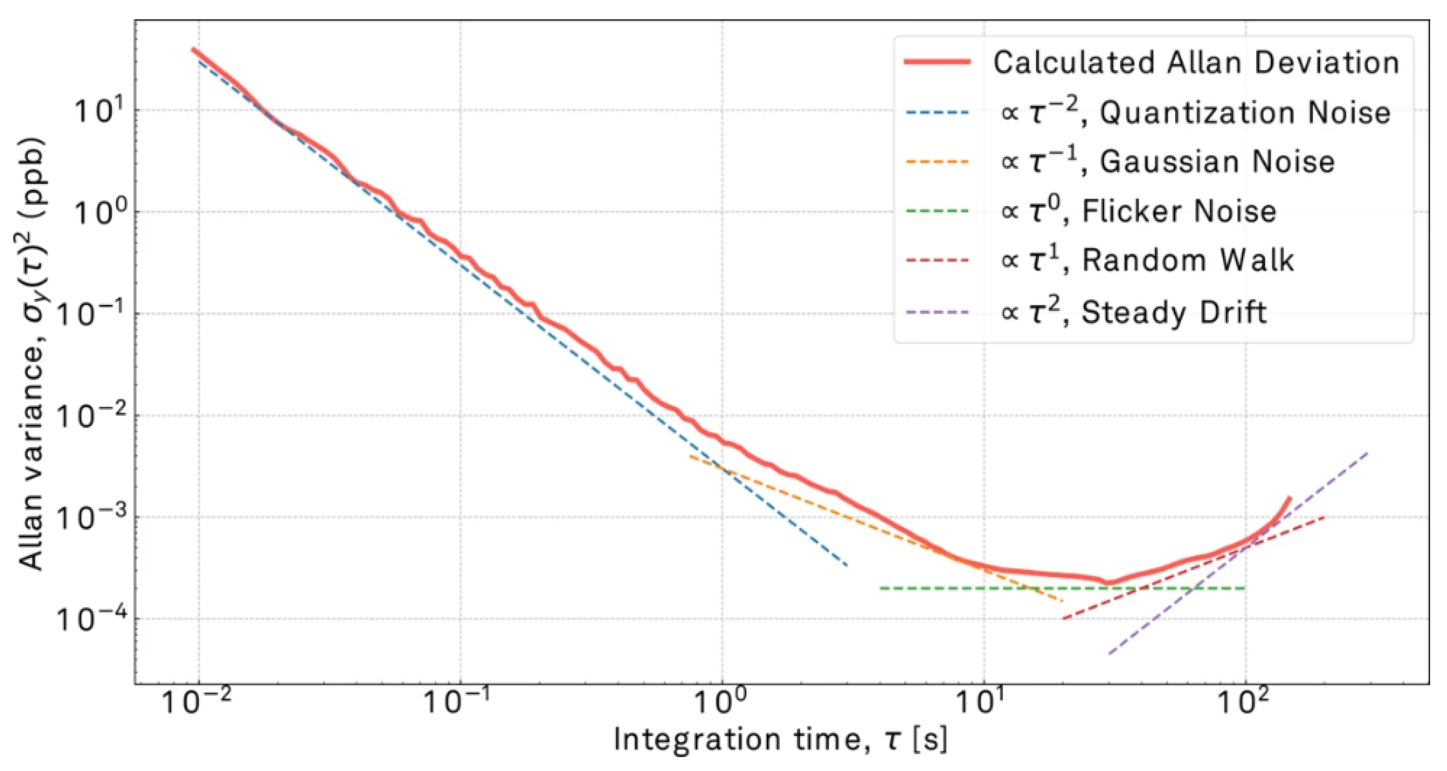
34], two asymptotes are unreasonably drawn, conjugating sections with a double and a zero slope. Indeed, if there are two conjugate sections on a double logarithmic scale, then the difference between the actual curve and the value at the intersection point of the asymptotes is 3 dB for a function to the first degree, or, accordingly, 6 dB for a quadratic function. When the leftmost asymptote is conjugated with the average asymptote, the deviation from the intersection point of the asymptotes does not exceed a decade, and when the rightmost asymptote is conjugated with the average asymptote, the deviation is even smaller, it does not exceed one third of a decade, so in this case the very existence of an asymptote with a positive double slope follows cast great doubt, especially since this deviation is barely noticeable on the graph of experimental points. Of course, the growth of this function in this case is caused by an increase in the experimental error or a lack of statistical data. Thus, this article gives another example from many similar examples when experimenters do not understand the essence of the random processes they are studying and follow the traditions that introduced these five types of slopes of the Allan function graph and assigned specific noise names to each of the slopes: quantization noise, Gaussian noise, flicker noise, random drift and continuous drift. Researchers are ready to see signs of these noises even where there are none. If the given plot shown in
Figure 18 is taken from experimental measurements, then only part of the interval
is credible. The graph for
is a graph of the error of the measuring device due to quantization inherent in the counting method of measurements. This error can be reduced by 1000 times through the use of technical solutions described in patents [
41], [
42]. As for the interval
, the growth of the Allan function in this interval can be reduced due to more careful measurements and the accumulation of more representative statistical data.
Nevertheless, there are measurement results in which, reliably for the dispersion, a negative slope of the second order turns into a negative slope of the first order, or, more correctly, a negative slope of the first order of the Allan function turns into a slope of the order of 0.5. This has its own natural explanation. At short time intervals, usually constituting
the average frequency value, it is measured by a counting method without stopping the counter. Therefore, there is an inversely proportional dependence of the measurement error by the counting method on the averaging time, i.e.,
. When averaging over time
or for some types of frequency meters when averaging over time,
the frequency meter does not provide the ability to continuously count pulses of the measured frequency over such a long interval, which is limited by the length of the counters. For this reason, the average frequency value is not measured directly experimentally for each report separately and correctly, but is calculated by averaging several successively obtained results. But since the counter stops, it is not the decrease in measurement error that is inversely proportional to the averaging time, but only statistical averaging. In this case, the dispersion of the measurement results is inversely proportional to the number of samples used in averaging, that is, the quadratic Allan dispersion function is inversely proportional to
, and since the Allan function (standard deviation) is the root of the dispersion, then for the Allan function this graph will have a slope inversely proportional to the root from
. So this asymptote begins where the measurement results are obtained not using continuous counting, but using the sum of the measurement results. If we use a frequency meter without dead time, as proposed in the patent [
42], then this function will continue to fall with the same slope, a multiple of the root of
, until this measurement error graph intersects the graph of the true instability of the generator under study, after then the decrease in this Allan function will stop, and the graph will reach an asymptote with a zero slope.
Appendix A. Some clarifications for readers
The variance and Allan function are also used to certify generators that do not claim to be a prototype of a frequency standard.
We are talking about quartz generators of the following types: OCXO, TCXO, CSAC. The author of the article is not engaged in the problem of certification, research or modification of quartz generators. The author of the article was engaged in the development of software and hardware for the certification of laser prototypes of frequency standards, as well as atomic prototypes of frequency standards. The mentioned generators of the OCXO, TCXO, CSAC types can be certified using more accurate generators called primary frequency standards. Such generators can be certified very simply using primary or secondary frequency standards, namely: to compare the frequency actually generated by them with the frequency that should be generated, using the frequency generated by a higher-order standard as a reference generator to measure this difference. For example, if the relative frequency drift of this generator, for example, over 30 days, is described by the value of 10 -14 Hz , then certification is carried out by comparing the relative drift of two identical generators of this type, which in this case is unjustified, since there are generators with a significantly lower value of this parameter. For example, a similar parameter of the primary standard is 10 -16 Hz .
To measure the relative frequency deviation from its starting value, it is sufficient to have only two identical generators that are being examined. But this is an excessive simplification of the certification method, when it is not the primary standard that is being certified, but the secondary one. It would be more reliable to compare the frequency of the generator being certified with any standard that is characterized by better frequency formation accuracy. And in this case, the question arises about what should be called the “accuracy” of the frequency standard. This question cannot be answered in the same way for the primary standard and for all other standards.
The answer to this question for all other standards is very simple: accuracy is the reciprocal of the relative error, and the relative error is the difference between the frequency value actually generated by this generator and the more accurate value that this generator should actually generate if it had an error no worse than the primary frequency standard. Metrological certification in this case could be carried out, for example, by mixing the frequencies of the generator being certified and the standard and measuring the difference frequency. In this case, to measure the difference frequency, the frequency obtained from the primary standard should be measured using the reference frequency.
Let’s assume that the primary standard generates a frequency of 9.192 GHz. The generator being certified generates a frequency of 100 MHz. It is enough to divide the frequency of the primary standard by 90 times, we will get 102.1 MHz, then multiply this frequency by the frequency of the generator being certified, we should get a difference frequency equal to 2.1 MHz.
Using the counting method, it is possible to measure this difference frequency with a relative error of about 10-16 , which is excessive for this task. Indeed, an error equal to 10-13 for a frequency of 100 MHz corresponds to a value of 1×10⁻⁵ Hz, which is a fraction of 0.5×10⁻¹¹ for a frequency of 2.1 MHz , that is five orders of magnitude greater than can be measured. Thus, the certification of any secondary standard and of a standard of an even lower level is merely an elementary engineering task; if it is not carried out, it is only because it is either not required, or is expensive, or, although desirable, is considered too complex and/or expensive.
The author of the article is not interested in the problem of certification of any secondary generators, this problem, strictly speaking, is not scientific, it is technical, engineering. For this reason, these issues are not considered in this article at all.
The author deals with the issues of certification of such generators that cannot be certified using more precise standards, since they claim to be prototypes of frequency standards. This means that their indicators are at least higher in some parameters than similar indicators of generally accepted frequency standards (or the frequency standard for a given country, at least).
Physicists are currently conducting research aimed at creating laser or atomic generators whose stability in terms of Allan parameters is estimated at 10-18 or less; there are reports of values of 10-19 being achieved , and for the implementation of projects to measure gravitational waves, for example, from the Crab Nebula, the need for a frequency standard with an error of 10-24 has been indicated.
The correct terminology is not always used in this area, since measurements may actually require only frequency stability, since we are talking about the sensitivity of metrological studies, and not about the accuracy of these measurements. If we were talking about accuracy, then the parameters characterizing not stability, but accuracy, should be applied to the reference generator.
Stability is relatively easy to measure even for a primary standard. Two identical primary standards should be used for this purpose. For example, if such a standard based on a He—Ne laser stabilized by the corresponding absorption lines of Methane generates a frequency equal to approximately 89 THz, i.e., 89×10 12 Hz, and the difference frequency, for example, is 10 Hz, then it is sufficient to measure the drift of this difference frequency over different time intervals. If the drift were 0.0001 Hz, for example, over 1000 s, then this value is 1.12×10 -18 . This value is better than the corresponding characteristic of the state frequency standard. Consequently, it is impossible to use the state frequency standard to detect this value, therefore such generators are certified relative to exactly the same generators, as if by themselves, autonomously, without using other metrological means of higher accuracy. As we can see, the characteristic of high stability can be extremely high, despite the fact that the actual difference in frequencies of two identical generators will be 10 Hz, which is 1.12×10 -13 .
For this reason, stability characteristics should be clearly distinguished from accuracy characteristics, just as accuracy characteristics are distinguished from sensitivity characteristics of measuring instruments.
For example, a laser is used to measure the difference in distances between mirrors in two different directions. The measurement error is 0.05% of the wavelength. In this case, the sensitivity of the method will be approximately this value. But if it is required to measure this distance accurately, then the stability of the wavelength in the air should be taken into account, and the absolute error will depend on a combination of factors consisting of a change in the laser generation frequency and a change in the refractive index of air due to changes in temperature, pressure, etc. Accordingly, if the wavelength is 0.6 μm, then the sensitivity of the method is 0.3 nm . If the relative instability of the laser radiation frequency is 1×10 -12 , then at a distance of 2 km, which will give an optical path of 4 km, the error can be 4 nm . In this case, the absolute error differs from the sensitivity by more than ten times, but the differences can be much greater.
In some cases, when only sufficient sensitivity of measurements is required, but there are no requirements for absolute accuracy, the experiment requires only the stability of the reference generator, but does not require its absolute accuracy. However, in cases where high accuracy is required, such measurements are called absolute measurements, then it is precisely the provision of high accuracy that is required, and not the provision of high stability of frequency generation. In this case, “stability” is an insufficient characteristic of the reference generator. It is necessary to know how much the value of the generated frequency differs from the value prescribed for it, this is described only by such a characteristic as the relative error (or its inverse value—accuracy), or the absolute error, equal to the product of the relative error and the measured value.
We offer translation of this page
Among the parameters characterizing the frequency stability, we find values of the order of one to the seventeenth digit. However, the value of the generated frequency itself is specified by a number in which only ten significant digits are indicated.
If the specified frequency standard produced the required frequency within the error limits corresponding to one sixteenth digit, then the value of this frequency should be standardized by a number that contains all sixteen significant digits of this value, i.e., the frequency value should be indicated with an accuracy of up to micro-Hertz units.
Now let’s get back to the topic of the article. If some point of the Allan function on the graph corresponds to a value of, say, 1.5×10⁻¹³ , say, for a time from 500 to 1000 seconds, but the right side of the Allan function graph has a positive slope, then we not only see that this graph, for example, reaches a value of 5.0×10⁻¹³ , according to the points shown on the graph, but we must also assume that with increasing time this value increases even more, for example, to values of 1.0×10⁻¹² and, perhaps, 1.0×10⁻¹¹ and so on. The conclusion is that if the Allan function graph demonstrates growth with increasing averaging time, then this graph does not prove absolutely nothing, no “long-term stability” attributed to this generator is a reliable characteristic of this generator, and it cannot be considered as a prototype of a future new frequency standard. Even if this characteristic goes in its right part parallel to the abscissa axis, this causes legitimate surprise. But the growth of this value with the growth of the averaging time causes categorical objections, that is, the allegedly presented “prototype of the frequency standard” should be rejected, or it should be noted that the studies of its positive properties were not carried out correctly enough or not fully enough.
This article does not claim to cover all the issues related to the study of frequency standards noise. The task is not set that way. Those researchers who set the task of finding the causes of noise in order to combat it or theorists who simply set the task of creating adequate models of these noises, of course, can and should discuss Barnes-Jarvis Power Law Noise and other noise components. The author did not aim to discuss noise theory; he headed a department whose task was to ensure correct measurement of frequency stability parameters. As a result of long and diverse studies, the author is of the opinion that stability itself, measured and demonstrated in the form of Allan function graphs, is an insufficient characteristic of the accuracy of the frequency standards being created. The author believes that if absolute accuracy is not compared or measured in any way, and even admits the impossibility of measuring absolute accuracy, with which such a characteristic as frequency “non-reproducibility” would be unambiguously associated, then at least special attention should be paid to the behavior of the Allan function in the right part of the graph, corresponding to an increase in the frequency averaging time. Proposals for an appropriate assessment are fairly simple and clear. If in the example considered above, when two identical generators, for example, stabilized lasers, demonstrate high frequency “stability”, but the specified difference frequency is much higher, then the value of the difference frequency itself should be taken into account. For example, it is possible to conduct an experiment on multiple switching on and off of two compared identical frequency standards, and if the difference in the frequencies generated by them is a random variable, it would also be legal to provide a mathematical expectation and variance for it. The author does not insist on a quantitative or qualitative increase in experimental studies of future frequency standards being created, but he draws the readers’ attention to the fact that the presence of a minimum point on the Allan function graph and the value of the Allan function at this minimum point are not as important as the behavior of the right side of this graph for assessing such a concept as “frequency stability”, and considering this graph from the position of its limit behavior as the averaging time tends to infinity makes sense at least in theory, while it is not proposed to build models of this noise, introducing such terms as “frequency aging” and so on, but it is sufficient to simply state the fact that the specified graph reaches an asymptote parallel to the ordinate axis, or an asymptote with a negative or positive slope. This, in the opinion of the author of the article, is a very important characteristic, although not sufficient, but a necessary characteristic of any generator claiming to be adopted as a prototype of a future frequency standard. In addition, the author aimed to identify obvious errors in some publications that are positioned by their authors as explanatory and even educational materials, such as the publication [
43] in the first version of the article. The author of this article does not understand that in the case of using automatic frequency control systems, measuring the Allan function for short time intervals is meaningless, since it is illegitimate and incorrect.
Future primary frequency standards should provide the greatest possible long-term stability and actual accuracy. The unreliability of the Allan variance is obvious, since it excludes from consideration the constant differences in the frequency values generated by different generators. If we created some other way of generating an exact frequency and claim that this way is better, which is the task of fundamental metrology in the direction of creating frequency, time and length standards, then formally it would be necessary to create a sufficient number of identical “standards”, which is called an “ensemble of generators”. All these standards should be included, and they should generate the frequency value required for the tasks of metrology. It would be easy enough to measure the differences in the actual generated frequency values, but the problem rests on the fact that a statistically reliable number of standards that could be called an “ensemble”, which is apparently clearly greater than ten, is practically never achievable in practice. In practice, only two prototypes are always available and their frequencies are compared. In this case, according to the ergodicity hypothesis, averaging over the ensemble is replaced by averaging over time, which is clearly not sufficiently substantiated. Identical standards can be in the same conditions with respect to the following factors: power sources, temperature, pressure, magnetic field, gravitational field, and so on. So there can be many factors that make these “frequency standards” change the frequencies they generate synchronously. Therefore, the difference in the frequencies they generate is an insufficient measure of the stability of each of them individually. But since the experimenters cannot offer anything better, they have to accept what they have. Thus, the difference in the frequencies of only two “frequency standards” is measured and the hypothesis is used that the resulting frequency discrepancy is generated by approximately comparable deviations of each of them from the ideal value. That is, it is assumed that the deviations of the two lasers are independent, and therefore the total contribution of each is calculated not as the sum of the contributions of each of them, but as a statistical sum, that is, the variances are summed up, the difference frequency is considered equal to the square root of the sum of the squares of the deviation of the frequency of each “standard” from the ideal value. On this basis, for example, if the difference frequency is 10 Hz, then this value is considered to be the result of a deviation of each standard by an amount equal to 7.07 Hz, i.e., the root of two less than 10 Hz.
We measure changes in optical frequency, which, if we take a rounded value for simplicity of reasoning, is about 100 THz, for which two beams of light from two identical lasers stabilized by a special very complex circuit are directed to a common photodetector, the difference frequency is transferred by special means to the carrier frequency, for example, equal to 1 MHz. We need to measure the deviations and stability of this frequency in Hertz, the result is the result of measuring the absolute difference in the frequencies of the two specified lasers, therefore the obtained difference can be attributed to the carrier frequency equal to 100 THz = 100,000,000,000,000 Hz, that is, ten to the 14th power Hertz. If the obtained deviations at the carrier frequency are 0.01 Hz, then when converted to the original frequency, this gives one sixteenth digit. The measurement method is a counting method with a refinement of 1000 times, which is described in the article. Due to this, an error equal to 0.001 Hz occurs when averaging over a time equal to 1 s, but in this case we are talking only about the component generated by the discreteness of the count. Accordingly, this error decreases with an increase in the averaging time inversely proportional to this time, i.e., for 10 seconds it is 0.0001 Hz and so on. It is important that the error of the measuring device is less than the value measured in the experiment. If a conventional counting method were used, then for a time of 1 s the error would be 1 Hz, and the required error value of 0.001 Hz would be achieved only when averaging over 1000 seconds. In this case, the error of the measuring device would be comparable and even greater than the error of the frequency standard prototype developed by our colleagues.
Figure A1 shows the Allan function graph from the publication [
43]. As we can see, the authors attribute the increase in the right branch of the graph to the presence of drift (red line), but they also claim that even after eliminating the drift, the increase in the right part of the graph remains, although not as strong (blue line). In a discussion with one of the authors, the hypothesis that the increase may be due to some measurement error or insufficient statistics was rejected.
Figure A1.
Allan function from publication [
43].
Figure A1.
Allan function from publication [
43].
Appendix B. Digital Frequency Counter Without Dead Time
We have developed firmware (i.e., hardware and software tool) consisting of a hardware part, a software part and a computer connected to the hardware part, into which the software part is loaded, which we called the “FreqLab Program”, which is an abbreviation of the full name “Frequency Laboratory”.
The frequency meter has the following characteristics, confirmed by certification [
2]:
Three channels for measuring frequency or time interval (period).
Software selection of operating mode.
-
Range of measured input signal frequencies:
Input signal—TTL level (or harmonic oscillations with an amplitude of at least 0.5 V and noise of no more than 50 mV ).
The rate of reflection acquisition is 1000 measurements / (channel × sec).
The error in determining the pulse front time (time resolution) is ~ 1 ns.
“Dead time” is zero.
Communication with a computer via COM port ( RS -232).
Power supply fro. +9V source—network adapter from 220V × 50Hz network.
Software—the author’s program “ FreqLab “, supplied on a CD.
Input resistance of measuring inputs 50 Ohm.
It is possible to use an external frequency standard generator of 5 MHz or 10 MHz (selection is provided by software)
The software guarantees all functions using notebook PC.
-
Error Δf the measurement of frequency fX on the interval τ (sec) is determined by the relation: , where δf— relative error of measuring, determined by the ratio: . Here
fL—leading frequency,
σRO—absolute error of the reference oscillator,
σС—absolute counting error, given by the ratio: .
In the period measurement mode, the error ΔT of the measurement period TX on the interval τ (sec) is determined by the relation: . In the case of using the measurement mode from the internal generator, the value of σ OG in the calculation should be taken as equal to 10-7.
The program’s user interface allows you to accept a file in real time, obtained during measurements, and also to view a previously received file in a mode simulating the receipt of data in real time.
The interface has a line menu, a graphical information display area, scale control, and scrolling along the time axis.
The device has three operating modes:
frequency measurement mode for one, two or three channels;
single channel period measurement mode;
phase difference measurement mode for two channels.
In addition, the following operating modes can be set for calculating functions and displaying the corresponding graphs:
a) oscilloscope,
b) chart recorder,
c) spectrum,
d) Allen function (on short, medium or long time intervals).
The elimination of dead time in the frequency meter developed by us is ensured by synchronizing the reading of the counters into the registers. For this purpose, a structure is used, a simplified view of which is shown in
Figure A2. Such a scheme allows reading the counter readings without stopping their counting. The operation of the synchronization trigger is illustrated by the signal diagrams shown in
Figure A3.
Figure A4 shows the counting pulses that will be formed in this case and used for counting.
Figure A5 shows the signals in the refinement circuit, which provides a 1000-fold reduction in the measurement error in accordance with the technical solutions described in the patents [41, 42].
Figure A6 shows the complete structure of the frequency meter without dead time and with a refinement of the measuring interval, which provides a 1000-fold increase in accuracy. Here, the refinement of exactly 1000 times was chosen for convenience; it was possible to implement a frequency meter with a refinement somewhat greater or somewhat lesser, which depends on the pulse stretch coefficient, but, of course, this has its limitations. Any further refinement is unreliable, since other factors will begin to influence the error, and it is not required, so this particular pulse stretch ratio was chosen.
Figure A2.
Structure of a digital frequency counter without dead time.
Figure A2.
Structure of a digital frequency counter without dead time.
Figure A3.
Trigger signal diagrams.
Figure A3.
Trigger signal diagrams.
Figure A4.
Frequency meter timing diagrams.
Figure A4.
Frequency meter timing diagrams.
Figure A5.
Clarification of the positions of the fronts of the measured frequency signal relative to the boundaries of the measurement intervals by generating correction pulses FD.
Figure A5.
Clarification of the positions of the fronts of the measured frequency signal relative to the boundaries of the measurement intervals by generating correction pulses FD.
Figure A6.
Digital frequency meter with clarification channel.
Figure A6.
Digital frequency meter with clarification channel.
Figure A7.
Pulse stretching circuit: C—comparator, Form I—current shaper.
Figure A7.
Pulse stretching circuit: C—comparator, Form I—current shaper.
Figure A8.
Signals in the stretch circuit: UC—voltage on the capacitor.
Figure A8.
Signals in the stretch circuit: UC—voltage on the capacitor.
Figure A9.
The appearance of the frequency meter developed and implemented in the experiment.
Figure A9.
The appearance of the frequency meter developed and implemented in the experiment.
Figure A10.
The example of the window of software “FreqLab” in the mode of the oscilloscope.
Figure A10.
The example of the window of software “FreqLab” in the mode of the oscilloscope.
Figure A11.
The example of the window of software “FreqLab” in the mode of the oscilloscope with the virtual ruler.
Figure A11.
The example of the window of software “FreqLab” in the mode of the oscilloscope with the virtual ruler.
Figure A12.
Example of the FreqLab software window in recorder mode.
Figure A12.
Example of the FreqLab software window in recorder mode.
Figure A13.
Example of the FreqLab sottware window in the mode of frequency deviations.
Figure A13.
Example of the FreqLab sottware window in the mode of frequency deviations.
Figure A14.
Example of FreqLab software window in real time mode (Short, Middle and Long Allan functions).
Figure A14.
Example of FreqLab software window in real time mode (Short, Middle and Long Allan functions).
Figure A15.
Example of FreqLab program window in period measurement mode.
Figure A15.
Example of FreqLab program window in period measurement mode.
Figure A16.
Example of a histogram window.
Figure A16.
Example of a histogram window.
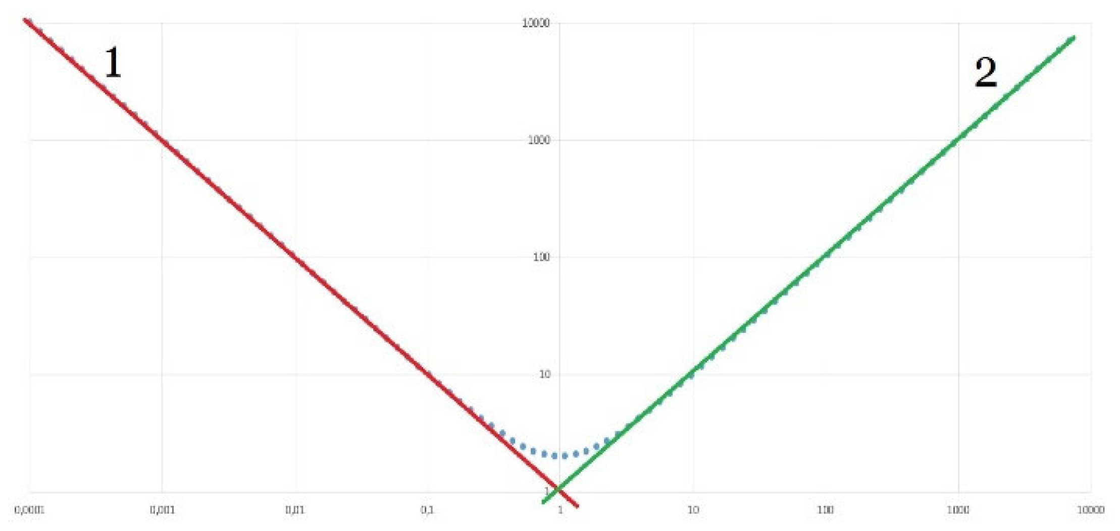
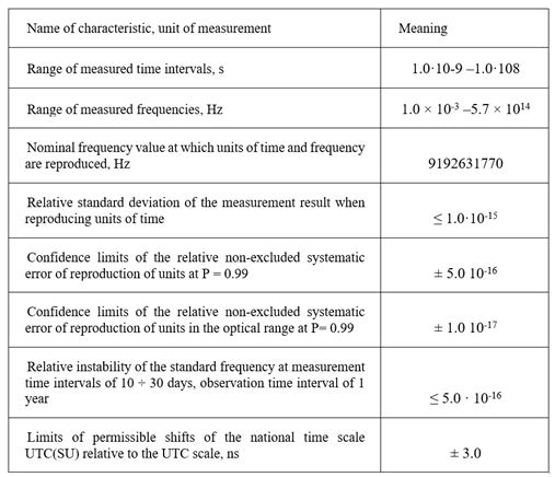
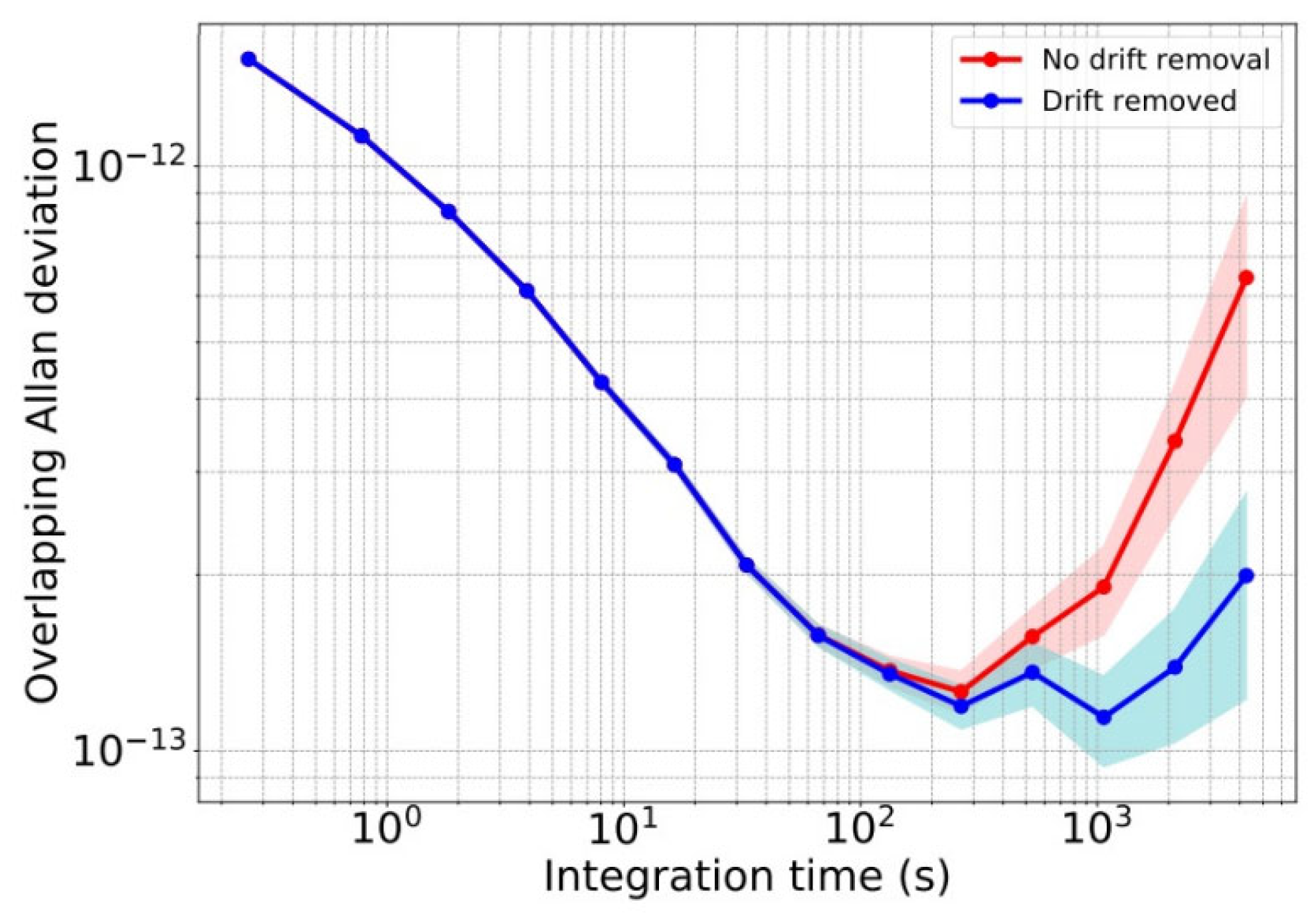
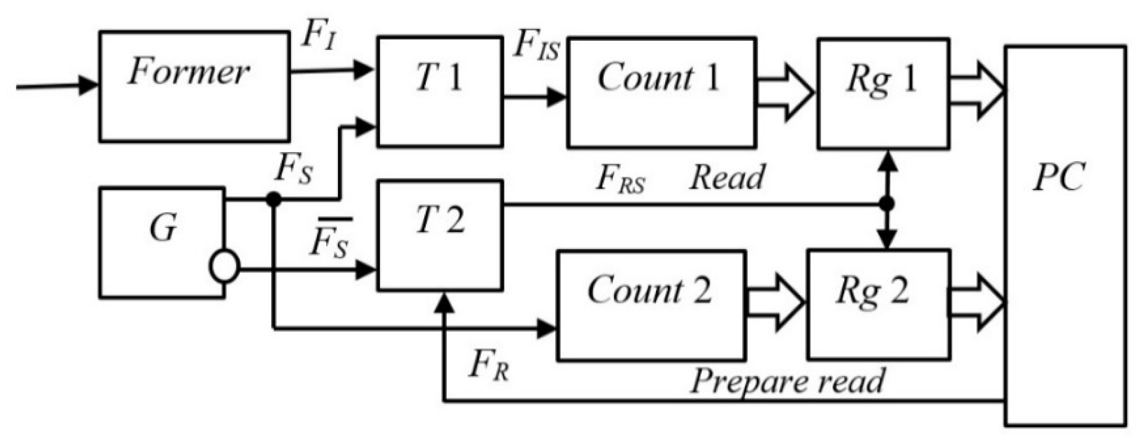

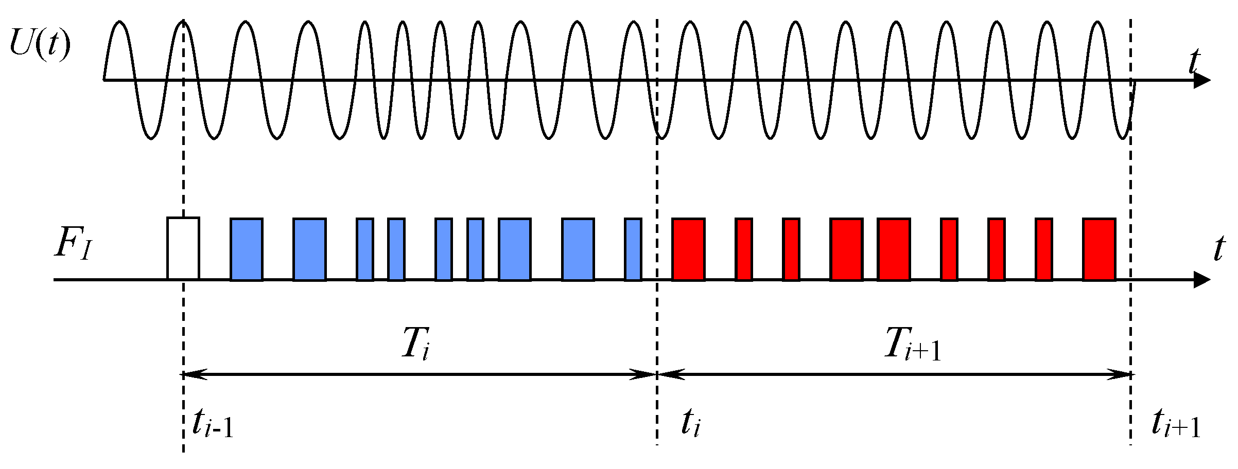
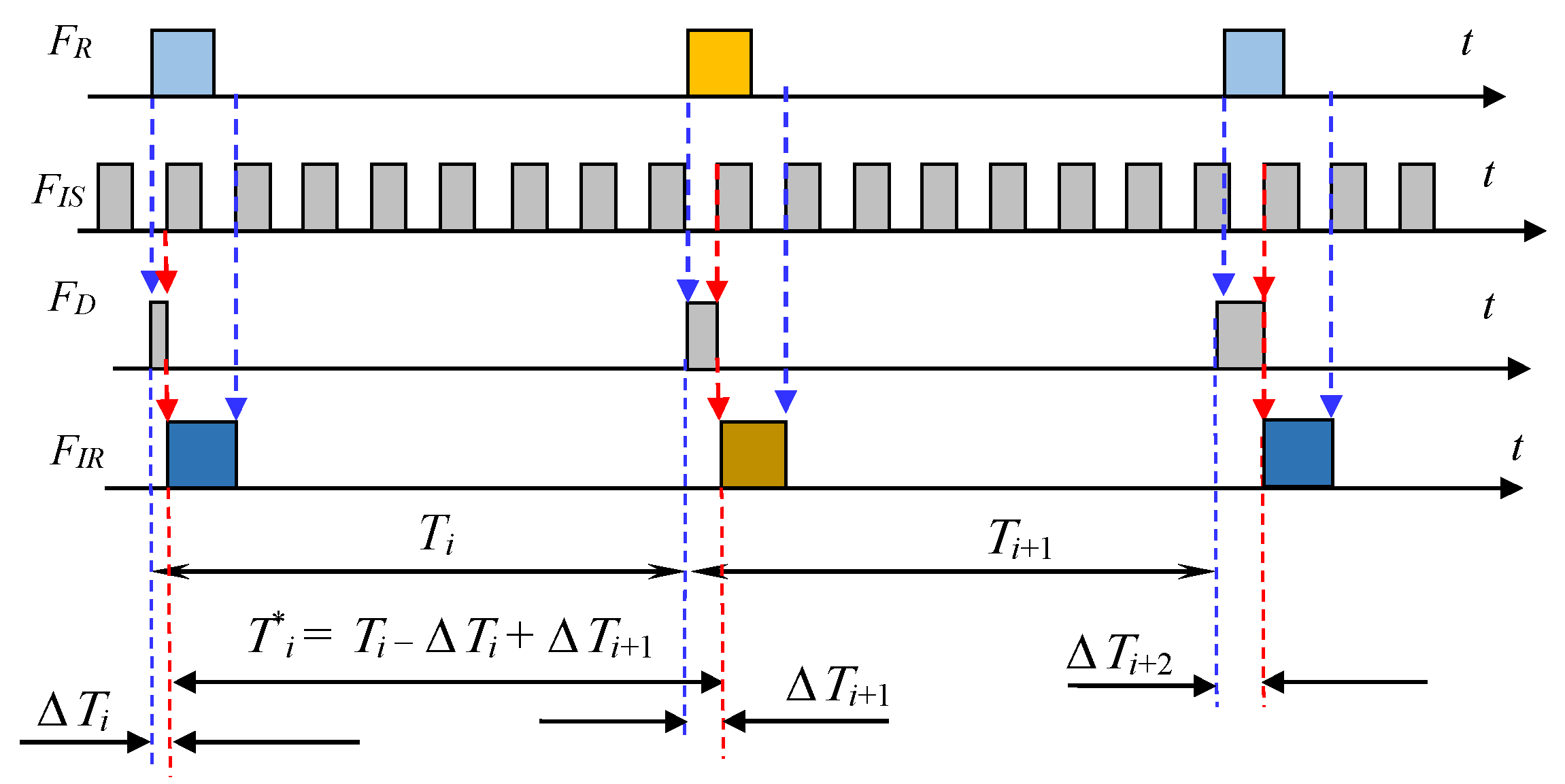
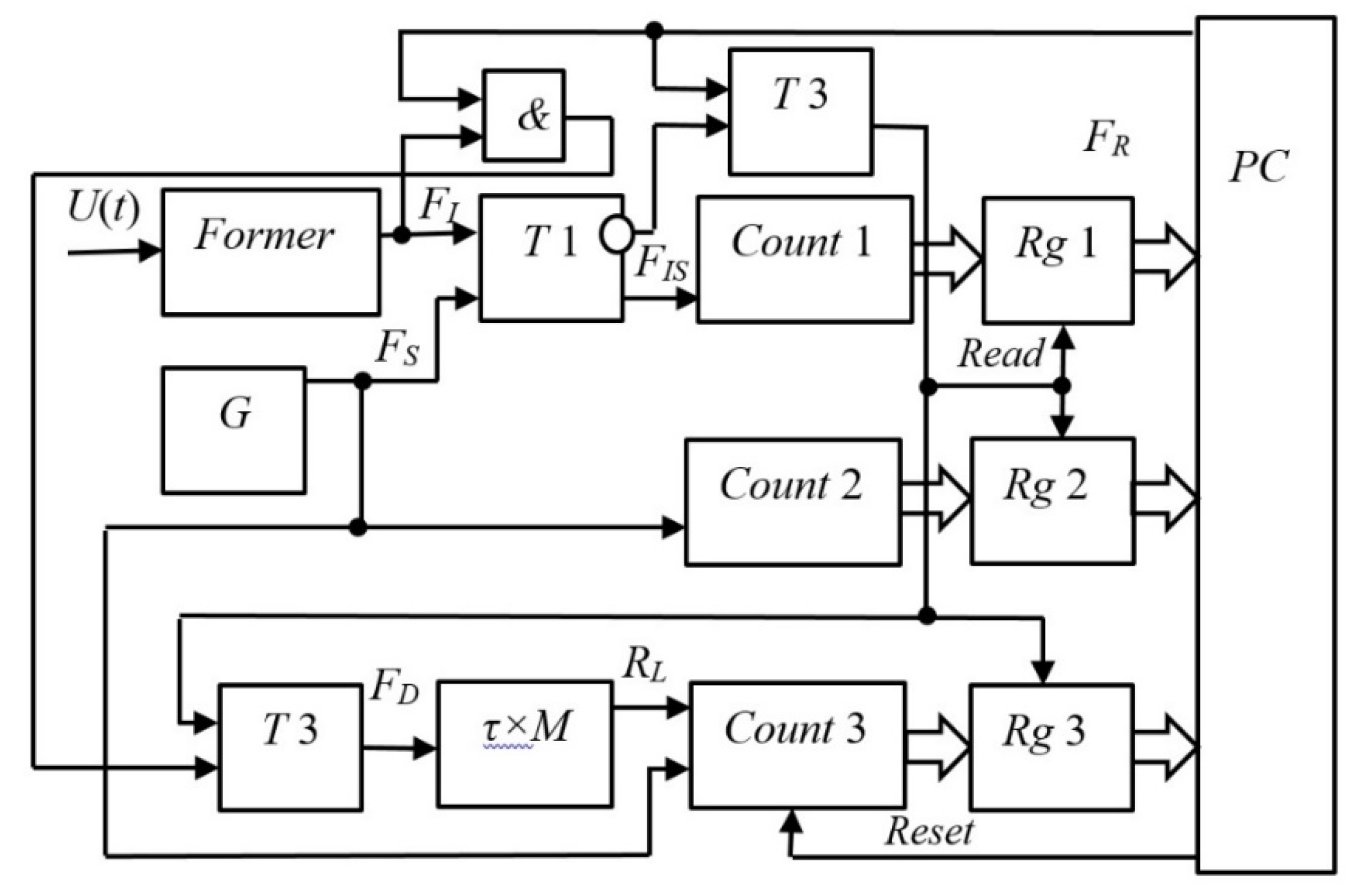

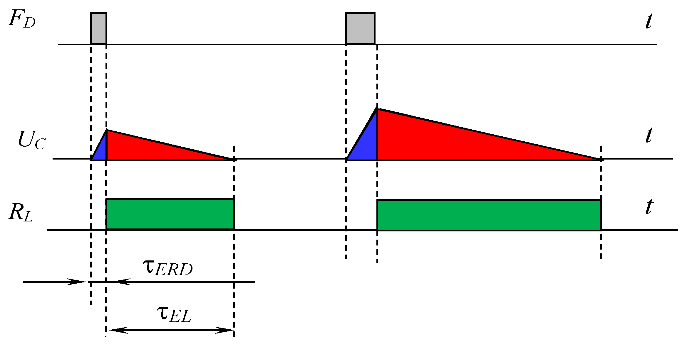
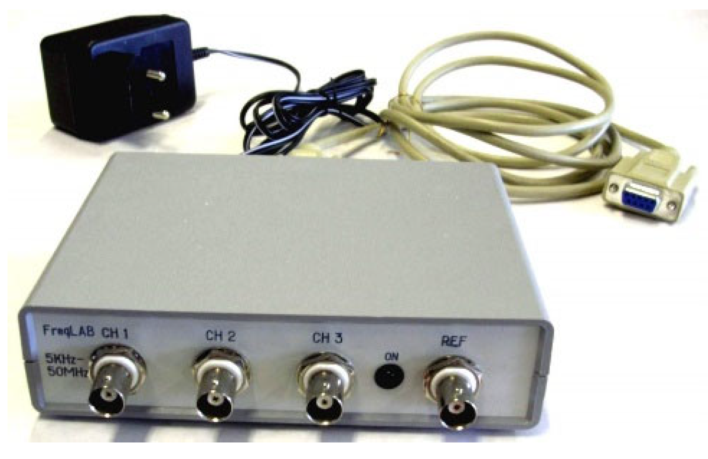
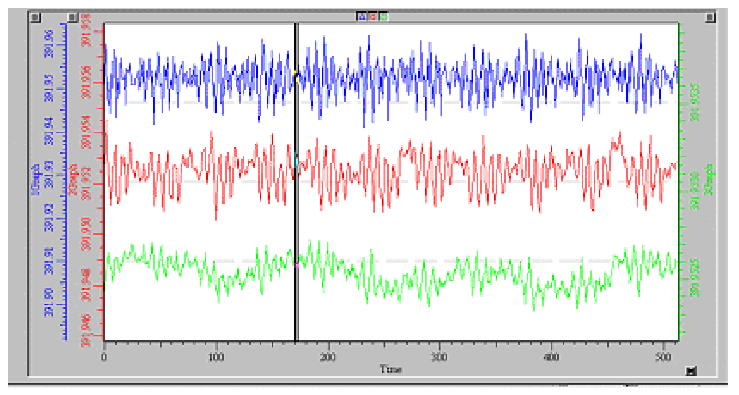
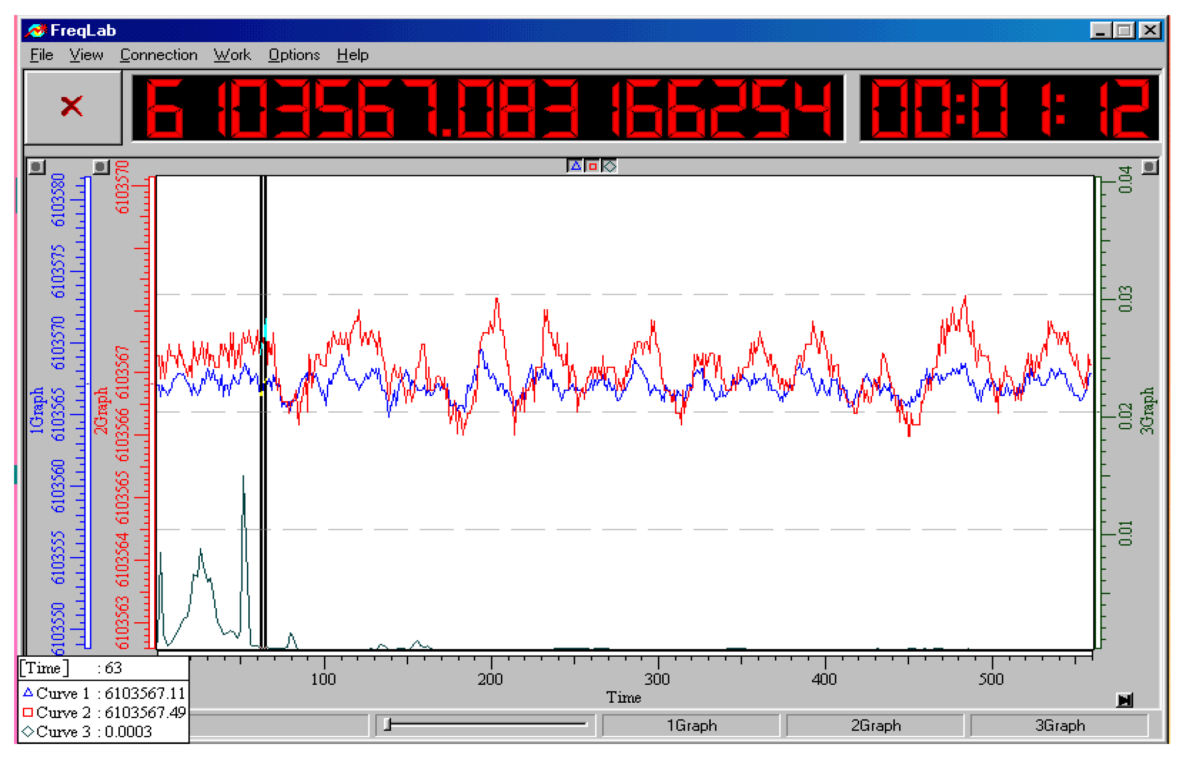
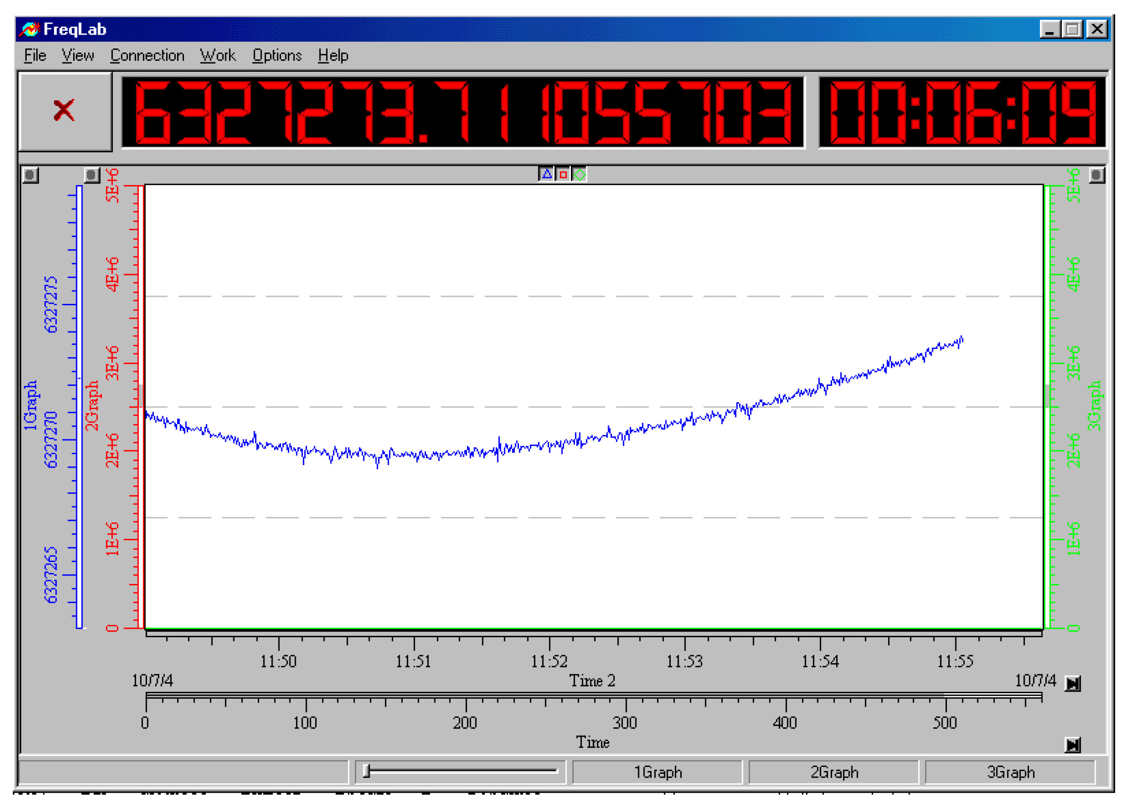
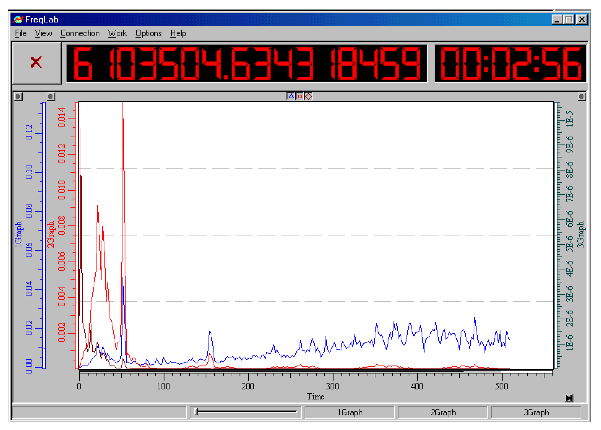
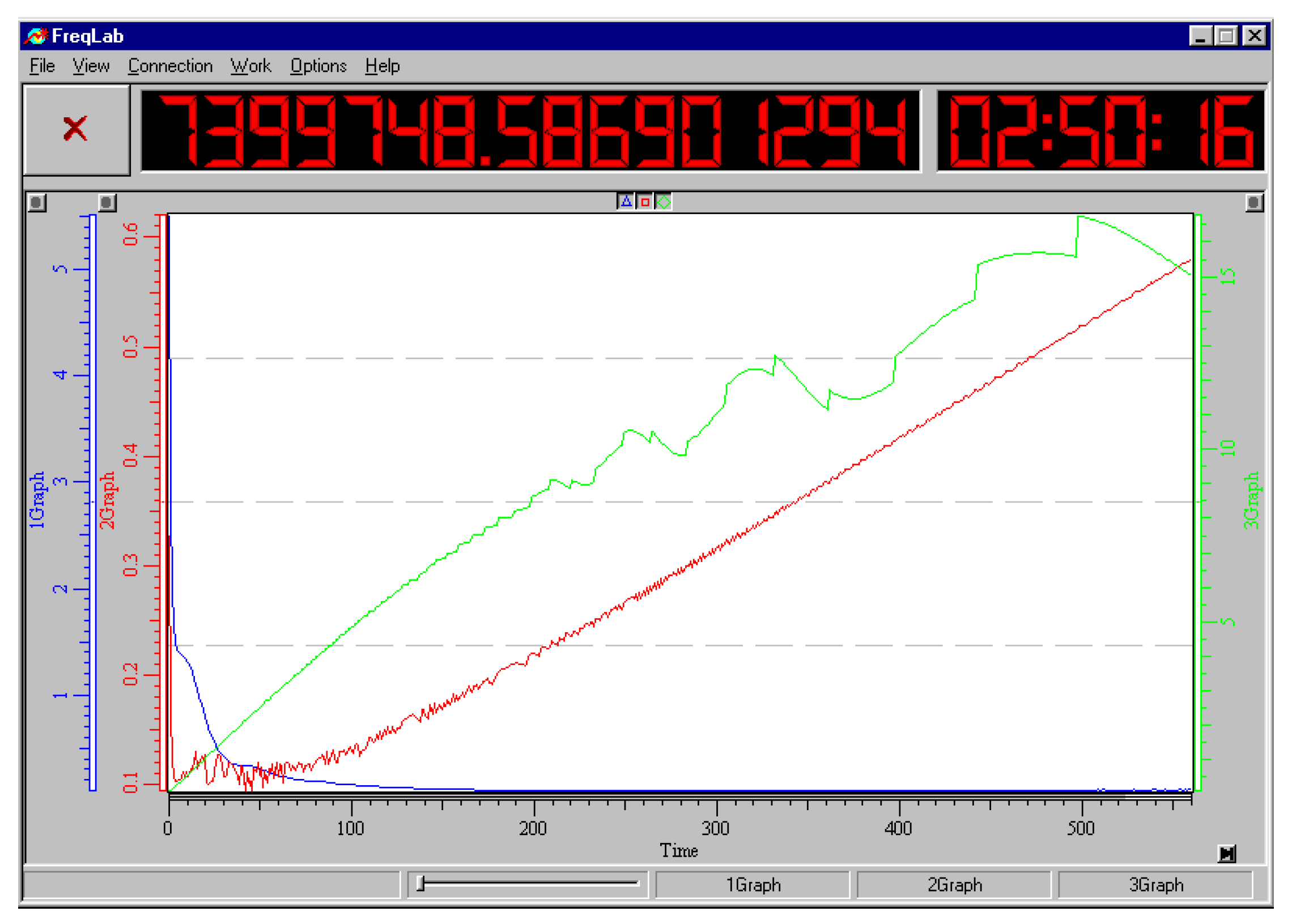
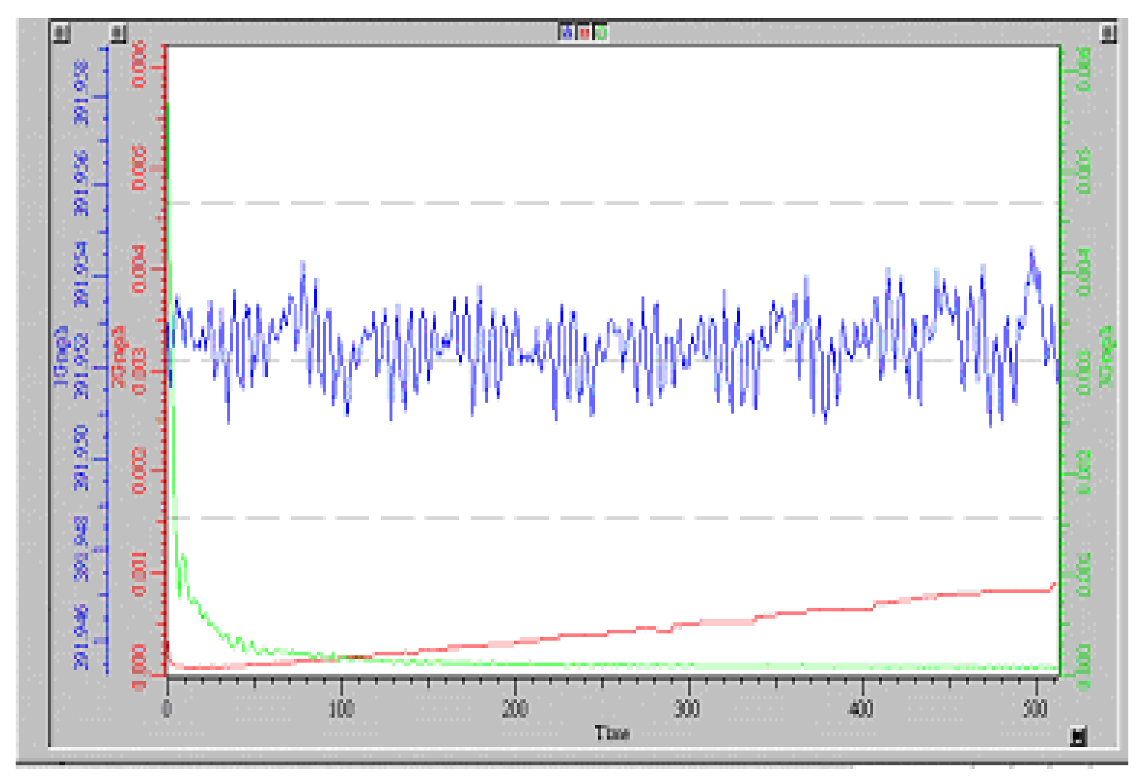
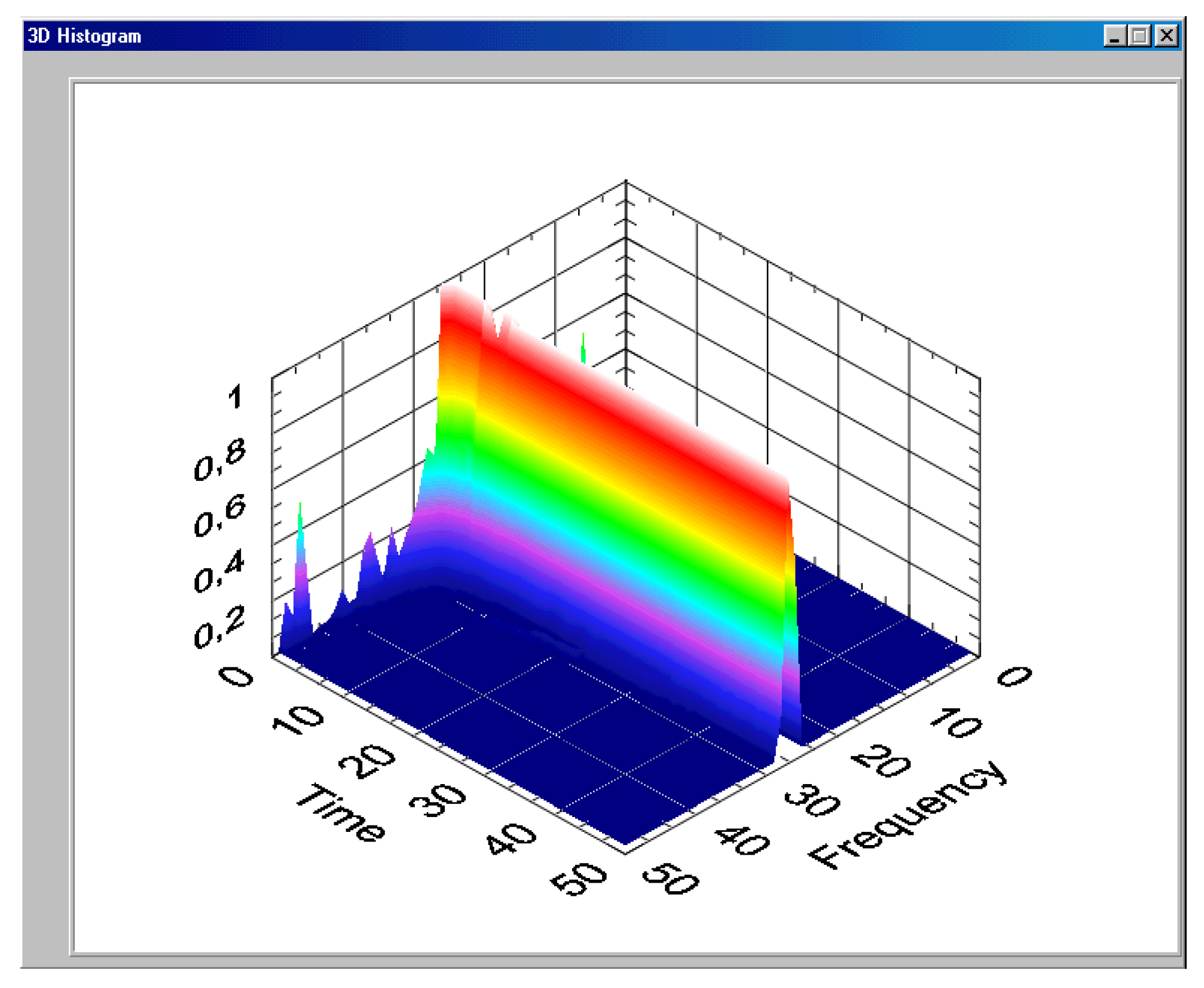


 was born 8-June-1959. He graduated Novosibirsk Electrotechnical Institute in 1981, grasuated PhD in Institute of Automatics and Electrometry in 1985. In 1981 he defended his diploma on “Synthesis of a PI controller for process control” in English with a rating of “excellent”, Diploma with honors G-1 No. 354335, qualified as an electrical engineer. Academic degrees and titles: The scientific degree of Doctor of Technical Sciences was awarded by a decision of the Higher Attestation Commission of January 16, 2004. Diploma DK No. 020425. Year: 2003. Degree: Doctor of Technical Sciences. Place of dissertation defense: Novosibirsk State Technical University. Specialty: Elements and devices of computer engineering and control systems. He is head of the Department of Laser Systems in Novosibirsk State Technical University, professor in Novosibirsk State University and in Siberean State Unoversity of Telecommunications and Informatis, foreing Professor in Al-Farabi Kazakh National University, Almaty, Kazakhstan, and in Eurasian National University after Gumilev, Astana, Kazakhstan. His main areas of interest: automation, mathematical modeling, optimization, laser physics, photonics, optoelectronics. He is a member of the editorial board of 12 international journals. He can be contacted at email: zhmud@corp.nstu.ru or oao_nips@bk.ru.

