Inverse Coefficient Problem for Epidemiological Mean Field Formulation

Preprint

Article

Inverse Coefficient Problem for Epidemiological Mean Field Formulation

Altmetrics

Downloads

Views

Comments

A peer-reviewed article of this preprint also exists.

Viktoriya Sergeevna Petrakova^*

This version is not peer-reviewed

Submitted:

08 October 2024

Posted:

08 October 2024

You are already at the latest version

Alerts

Abstract

The paper proposes an approach to solving the inverse epidemiological problem, written in terms of the “mean field” theory. Finding the coefficients of the epidemiological SIR mean field model is reduced to solving an optimization problem, for the solution of which only zero-order methods can be used. The Nelder-Mead method was chosen as such a method. The algorithm for solution of the inverse coefficient problem is proposed. Computational experiments were carried out to compare the obtained solutions with respect to synthetic and real data. The results of computational experiments have shown the efficiency of this approach. Ways to further improve the approach have also been determined.

Keywords:

Subject: Computer Science and Mathematics - Mathematical and Computational Biology

1. Introduction

The coronavirus epidemic, which was spreading most in 2020-2022, has shown the need to develop measures to contain the spread of the disease due to reduce mortality among the population and the burden on the healthcare system. At the same time, the measures introduced can vary quite significantly: from the development of a hand-washing culture to complete long-term isolation, be perceived by society differently [1,2,3,4] and have different effects on the economy and other areas of public life. Methods of mathematical modeling help to assess the consequences of decisions taken at different levels. At present, models of optimal control of various kinds are being significantly developed, since this approach is more flexible and allows us to assess the sensitivity of the modeled system to the slightest changes in the choice of the population behavior strategy and the external planner. Thus, using the basic epidemiological model of the SIS, in [5] an optimal management model is proposed in which the planner uses tax revenues to direct funds either to preventive measures for the population or to treatment of the infected. By analyzing the social costs of prevention and treatment, the authors determine the policy that is most cost-effective in different situations. In [6] a “mean-field model” is proposed, based on the premise that the selfish actions of each individual are likely to maximize personal utility, as opposed to a socially optimal strategy that maximizes the total utility for the entire population. The authors assume that the reduction of contacts with infected people should continue long after the epidemic has subsided.

One approach to modeling the dynamics of epidemic spread is optimal control models written in terms of “mean field” theory. Here it is assumed that the population is large enough and the influence of the strategy adopted by an individual is negligible and does not affect the overall behavior of the population. This assumption allows one to pass to the limit in explicit agent-based modeling problems and describe the behavior of the population with a small number of equations. One of the epidemiological mean field models will be discussed in more detail in Section 2.1. We also note the paper with a review of the use of various mean field approaches for modeling the dynamics of epidemics [7]. Previously, the studies [8,9] demonstrated the advantage of mean-field predictive models over commonly used compartmental SIR-type models.

The need to solve inverse problems for various mathematical epidemiological formulations is caused by the presence of statistical data (usually noisy) describing the dynamics of disease development and a large set of parameters in the mathematical model used for forecasting. The parameters being reconstructed are usually physical, but difficult to determine, since they depend on a large number of factors. For example, the contagiousness parameter (the rate of virus spread), used in the overwhelming majority of epidemiological models, depends on the infectiousness of the virus, the frequency of contacts in the population, the incubation period of the virus, and compliance with anti-virus restrictions.

There are only a few papers on solving inverse mean field problems [10,11,12]. These papers consider classical formulations in the form of a system of two partial differential equations, used mainly to solve economic problems. The problems of finding solutions of inverse problems for mean-field models arise due to the strict restrictions on the choice of the cost functional describing the behavior of the system to ensure the existence and uniqueness of the solution of direct problem. Such conditions for epidemilogical mean field formulation are discussed in more detail in Section 2.2. To overcome them, in [10], for example, the continuity equation is considered instead of the Fokker-Planck one, which is used in mean-field systems to describe the evolution of the population. This assumption leads to the fact that with zero current costs and a certain type of terminal conditions, the formulation is similar to the transfer optimization problem, for which the inverse problem has been already solved. The papers [11,12] consider the reconstruction of the Hamiltonian of the classical mean-field model based on a limited set of noisy partial observations of population dynamics with a limited aperture. To achieve this goal, the authors formalize the inverse problem as an optimization problem with constraints on the residual functional using the least-squares method with appropriate norms. The Chambolle-Pock method (a variation of the gradient method) is used to solve the inverse problem. The authors note that due to the strong incorrectness of the formulation, it is very difficult to obtain a high-quality reconstruction.

This work is aimed at solving practical problems arising from epidemiological modeling. Here, to remain within the framework of the uniqueness of the existence of a solution to the direct problem, an inverse coefficient problem is formulated. The inverse problem is formulated as a multicriterial optimization problem with constraints, which can only be solved by zero-order methods. Sections “Materials and Methods”, “Results” and “Discussion” present computational experiments on reconstruction of model parameters on synthetic and real data.

2. Mathematical Formulation

2.1. Direct Problem

As a direct mean field problem it is used the formulation which was first introduced in [13] and called the SIR Mean Field model with Total Control for all epidemiological Groups (SIR TGC MF model). This formulation differs from the one proposed, e.g, in [14], by the generality of the chosen strategy for the entire population. Their comparison is given in the work [13]. The formulation of a direct problem is the following:

find the minima of the cost functional

\begin{matrix} J (m_{S I R}, α) = \int_{0}^{T} & \int_{0}^{1} (\sum_{i \in {S, I, R}} G_{i} (m_{S I R}, α) m_{i} + \\ + g (t, x, m_{S I R})) d x d t + \int_{0}^{1} Φ (m_{S I R} (T, x)) d x \end{matrix}

(1)

with restrictions in the form of the system of convection-diffusion equations

\{\begin{matrix} \begin{matrix} \partial_{t} m_{S} + \nabla (m_{S} α) + β m_{S} m_{I} - σ_{S}^{2} Δ m_{S} / 2 = 0, \end{matrix} \\ \begin{matrix} \partial_{t} m_{I} + \nabla (m_{I} α) - β m_{S} m_{I} + γ m_{I} - σ_{I}^{2} Δ m_{I} / 2 = 0, \end{matrix} \\ \begin{matrix} \partial_{t} m_{R} + \nabla (m_{R} α) - γ m_{I} - σ_{R}^{2} Δ m_{R} / 2 = 0 \end{matrix} \end{matrix}

(2)

with initial

m_{i} (0, x) = m_{0 i} (x) on Ω

(3)

and Neumann boundary conditions

\partial m_{i} / \partial x = 0 \forall t and x \in Γ_{Ω} .

(4)

Here the stochastic processes within the population are described using non-negative parameters

σ_{i}

i \in {S, I, R}

;

m_{i} (t, x) : [0, T] \times Ω \to R

are the functions presenting the distribution of individuals in each epidemiological group

i \in {S, I, R}

over the state space

Ω

at each time moment

t \in [0, T]

. State variable x indicates the population’s loyalty to quarantine measures;

x = 0

is the agent’s dedication to the imposed restriction measures and

x = 1

is the opposite. Functions

α_{i} (t, x) : [0, T] \times [0, 1] \to R

i \in {S, I, R}

denote the compliance strategy of the representative agent of each group in the population.

The using of Lagrange multiplayer method for optimization problem (1)–(4) leads to the conjugate system of partial differential equations

\{\begin{matrix} \begin{matrix} \partial ψ_{S} / \partial t + {σ_{S}}^{2} Δ ψ_{S} / 2 & + α \cdot \partial ψ_{S} / \partial x + β m_{I} (ψ_{I} - ψ_{S}) = \\ = - \sum_{i \in {S, I, R}} m_{i} \partial G_{i} / \partial m_{S} - G_{S} - \partial g / \partial m_{S}, \end{matrix} \\ \begin{matrix} \partial ψ_{I} / \partial t + {σ_{I}}^{2} Δ ψ_{I} / 2 & + α \cdot \partial ψ_{I} / \partial x + β m_{S} (ψ_{I} - ψ_{S}) + γ (ψ_{R} - ψ_{I}) = \\ = - \sum_{i \in {S, I, R}} m_{i} \partial G_{i} / \partial m_{I} - G_{I} - \partial g / \partial m_{I}, \end{matrix} \\ \begin{matrix} \partial ψ_{R} / \partial t + {σ_{R}}^{2} Δ ψ_{R} / 2 & + α \cdot \partial ψ_{R} / \partial x = \\ = - \sum_{i \in {S, I, R}} m_{i} \partial G_{i} / \partial m_{R} - G_{R} - \partial g / \partial m_{R} \end{matrix} \end{matrix}

(5)

with the conditions on time horizon

ψ_{i} (T, x) = \frac{\partial Φ}{\partial m_{i}} (T, x) \forall x \in [0, 1], \forall i \in {S, I, R}

(6)

and the boundary conditions

\partial ψ_{i} / \partial x = 0 \forall t and x \in Γ_{Ω} .

(7)

In addition to conjugate system the optimal conditions on

α

function shoud be satisfied for

\bar{α} \in R

\forall (t, x) \in [0, T] \times [0, 1]

\sum_{j \in {S, I, R}} m_{j} (\frac{\partial G_{j}}{\partial \bar{α}} + \frac{\partial ψ_{j}}{\partial x}) = 0 .

(8)

Note, that systems (4)–(6), (8) are valid when the following conditions are performed:

α (t, 0) = α (t, 1) = 0 \forall t \in [0, T] .

(9)

Thus, the set of systems of equations (2)–(9) describes the optimum of a dynamic system, the evolution of which is determined by the cost function (1).

2.2. Inverse Problem Formulation

The main difficulties of the solution of the mean field problem used for real-life application is based on the strict restrictions on the domain of the existence and uniqueness of the solution. The most general condition for meeting these needs is the convexity of the functional with respect to the control variables. In paper [13] these restrictions are formulated for the SIR mean field problem with individual control for each epidemiological group (see Property 4 in [13]). Below reformulation of these restrictions is proposed for the SIR TGC MF model (2)–(9) used in this study.

Property 1. [Reformulation of Property 4 [13]] Conditions for the existence and uniqueness of a weak solution of the SIR TGC MF model. Assume that running cost function

G_{i}

grows quadratically with respect to control function

α

and the following conditions are satisfied:

\begin{matrix} \exists M > 0 : (\frac{\partial G_{i}}{\partial α} (m_{S I R}, α) - \frac{\partial G_{i}}{\partial α} (m_{S I R}, α)) \cdot (α - \tilde{α}) > 0 \\ \forall α, \tilde{α} : α \neq \tilde{α}, whenever |\frac{\partial G_{i}}{\partial α}|, |\frac{\partial G_{i}}{\partial \tilde{α}}| > M . \end{matrix}

(10)

Assume that g,

Φ

are non decreasing with respect to m, bounded below and satisfy

\begin{matrix} \forall L > 0 g_{L} : = sup_{m \in [0, L]} |g (t, x, m)| \in L^{1} ((0, T) \times Ω), \\ \forall L > 0 Φ_{L} : = sup_{m \in [0, L]} |Φ (T, x)| \in L^{1} (Ω), \\ f_{i} \in L_{1} ((0, T) \times Ω), \forall i \in {S, I, R}, \end{matrix}

(11)

where

f_{i}, i \in {S, I, R}

are the right parts of (2):

f_{S} = - β m_{S} m_{I}; f_{I} = β m_{S} m_{I} - γ m_{I}; f_{R} = γ m_{I} .

(12)

Then, for any

m_{0 i} \in L^{\infty} {(Σ)}_{+}

such as

log m_{0 i} \in L^{1} (Ω)

, there exists unique weak solution

(m_{S I R}, ψ_{S I R})

to the system of (2)–(9).

Thus, we are quite strongly limited by the area in which a unique solution to the direct problem exists. At the same time, the study of the difference in the sensitivity of the modeling results to the parameters of the model for formulation of the mean field problem and in the form of a system of ordinary differential equations of the SIR type for describing the epidemiological process shows that the main contribution to the dispersion of the output is made by the change in the epidemiological parameters of the model (parameters of contagiousness

β

and recovery

γ

). In Figure 1 the result of the sensitivity analysis is proposed. This result was first presented in the author’s previous work [13], but will be repeated here because it is important. Here the modeled number of infected people (I group) was used as output. For the input parameters, the following vector was used:

\begin{matrix} \vec{q} = (β, γ, I_{0}, σ_{S}, σ_{I}, σ_{R}, x_{S}^{c}, x_{I}^{c}, x_{R}^{c}, σ_{S}^{c}, σ_{I}^{c}, σ_{R}^{c}) . \end{matrix}

(13)

Here

x_{S}^{c}, x_{I}^{c}, x_{R}^{c}, σ_{S}^{c}, σ_{I}^{c}, σ_{R}^{c}

characterize the initial distribution of each epidemiological part of the population by the following way:

m_{0 i} = \frac{A_{i}}{B_{i}} (exp (- \frac{{(x - x_{i}^{c})}^{2}}{2 {(σ_{i}^{c})}^{2}}) / σ_{i}^{c} \sqrt{2 π} + a_{i} x^{2} + b_{i} {(1 - x)}^{2}) \forall i \in {S, I, R},

(14)

where

A_{i}

is the proportion of the current group in relation to the total population at the initial time;

B_{i}

is the normalization coefficient equal to the integral over

Ω

of the expression in brackets;

a_{i} = exp (- {(1 - x_{i}^{c})}^{2} / 2 {(σ_{i}^{c})}^{2}) (1 - x_{i}^{c}) / (2 {(σ_{i}^{c})}^{3} \sqrt{2 π})

and

b_{i} = exp (- {(x_{i}^{c})}^{2} / 2 {(σ_{i}^{c})}^{2}) (x_{i}^{c}) / (2 {(σ_{i}^{c})}^{3} \sqrt{2 π})

are the expressions which ensure boundary conditions (4) for

m (0, x)

. Physically, this means that we define the initial distributions as Gaussian (though with some small correction to comply with the boundary conditions). The parameter

I_{0}

is the proportion of the current group in relation to the total population at the initial time for the infected group. Here

A_{I}

coincides with

I_{0}

. For the estimation of sensitivity, the Extended Fourier Amplitude Sensitivity Test (eFAST)[15] was used. Method eFAST allows to divide the total variance of model output into components, corresponding to the model’s input parameters. The variance caused by any given parameter and their interaction is quantified by sensitivity indices being measurable indicators of the model’s sensitivity to parameter identification. The amplitude of sensitivity indices is presented in Figure 1. The inscriptions in the figure correspond to the order in which parameters are written, defined in (13), so ’sig_S’,’sig_I’,’sig_R’ correspond to model parameters

σ_{S}, σ_{I}, σ_{R}

; ’E_S’,’E_I’,’E_R’ for

x_{S}^{c}, x_{I}^{c}, x_{R}^{c}

and ’disp_S’,’disp_I’,’disp_R’ for

σ_{S}^{c}, σ_{I}^{c}, σ_{R}^{c}

Thus, based on the assumption that the epidemiological parameters are key for model (2)–(9), for real applications, the inverse coefficient problem is considered, instead of recovering the functions as was done in [10,11,12]. The idea here is to put

G_{i} (m_{S I R}, α) = a_{c} \frac{α^{2}}{2} m_{i}; g (t, x, m_{S I R}) = m_{I}^{2} (t, x); Φ (m_{S I R} (T, x)) = b_{c} m_{I}^{2} (T, x)

(15)

in direct problem functional (1). Here the

a_{c}

b_{c}

are unknown parameters.This choice is due to several reasons. First, assuming that the functions

G_{i}, g, Φ

are quadratic in control and the distribution densities, we remain in the domain of existence and uniqueness of the solution to the direct problem. Second, a very general assumption is made here about the development of the epidemic - the population acts in such a way (or is subject to such actions on the part of the government) to reduce the number of infected (choice of function g).

Then the inverse problem is: find the unknown coefficients

\vec{θ} = {β, γ, a_{c}, b_{c}}

which minimize the folliwing function:

min_{\vec{θ}} L = \sum_{q} {(\int_{0}^{1} m_{I} (q, x) d x - I_{q})}^{2} + \sum_{p} {(\int_{0}^{1} m_{R} (p, x) d x - R_{p})}^{2} .

(16)

Here

I_{q}

and

R_{p}

are known measures of infected and recovered parts of the population in some moments of time, determined by

p, q

the number of which is known in advance. Thus, in the considered formulation we optimize both the epidemiological component (through parameters

β, γ

) and the description of the population (parameters

a_{c}, b_{c}

3. Materials and Methods

3.1. Nelder-Mead Optimiaztion Method

Here, the Nelder-Mead method is used to solve the optimization problem. In 1965 [16], the Nelder-Mead (N-M) sequential optimization method was proposed as a direct method for local optimization of unconstrained problems and was a modification of the simplex method. The idea of the method is to compare the values of the objective function at

(n + 1)

vertices of the simplex and move the simplex towards the optimal point using an iterative procedure, where n is the number of model parameters to be reconstructed. In the original simplex method, a regular simplex was used at each stage. Nelder and Mead proposed several modifications of this method that allow simplices to be irregular. The result was a very reliable direct search method, which is one of the most effective if

n \leq 6

. Its effectiveness in practical applications has been demonstrated by the rapid initial decrease in the function values [17,18]. Recently, this well-known algorithm has been used in combination with global search algorithms such as random search [18] and genetic algorithm [19].

The implementation of the algorithm involves calculating the values of the objective function (defined here as (16)) at the vertices of simplex. Depending on the obtained values, the simplex changes the worst point from the set to a new one, which is closer to the local minimum. In a sense, the simplex creeps to the minimum value in the region. The condition for the termination of the iterative process is the smallness of the sides or area of the simplex obtained at the next iteration.

3.2. The Algorithm for the Solution of the Coefficient Inverse SIR MF Problem

Thus, for the constructed coefficient inverse problem, the following algorithm can be used.

Algorithm

Choose the initial value of vector $\vec{θ}$ being restored and the restrictions on the search area of each component of $\vec{θ}$ . Denote the obtained initial vector as ${\vec{θ}}^{0}$ ;
Put number of iteration k equaled zero ( $k = 0$ );
Solve the direct SIR MF problem (2)–(9),(15) with known parameters ${\vec{θ}}^{k}$ ;
Put $k = k + 1$ ;
Compute the $2 \cdot | {\vec{θ}}^{k} | + 1$ value of target function (16) on kth iteration at a small deviation from each vertex of the simplex under study. Do the iteration of Nelder-Mead algorithm and find new vector ${\vec{θ}}^{k}$ ;
Check the stopping criterion of the optimization method. If it is satisfied, then set $θ^{k}$ as the desired solution to the optimization problem; otherwise, return to step 3.

The solution of the direct problem of SIR MF was done using the finite difference approximation proposed in [13].

3.3. The description of computational experiments

The paper proposes two types of computational experiments: on synthetic and real data. Below is a description of each computational experiment.

Experiment №1

For the first experiment, we will compare the recovery possibility of only the

β

and

γ

parameters. As a set of synthetic data, we will consider the solution of a simple differential SIR model of the form

\begin{matrix} \{\begin{matrix} d m_{S} / d t = - β m_{S} m_{I}, \\ d m_{I} / d t = β m_{S} m_{I} - γ m_{I}, \\ d m_{R} / d t = γ m_{I} \end{matrix} \end{matrix}

(17)

with initial values

m_{S} (0) = S_{0}; m_{I} (0) = I_{0}; m_{R} (0) = R_{0}

and parameters describing the population and epidemiological process by the following way:

N = 1000, S_{0} = 800 / N, I_{0} = 200 / N, R_{0} = 0, β = 0.7, γ = 0.3 .

(18)

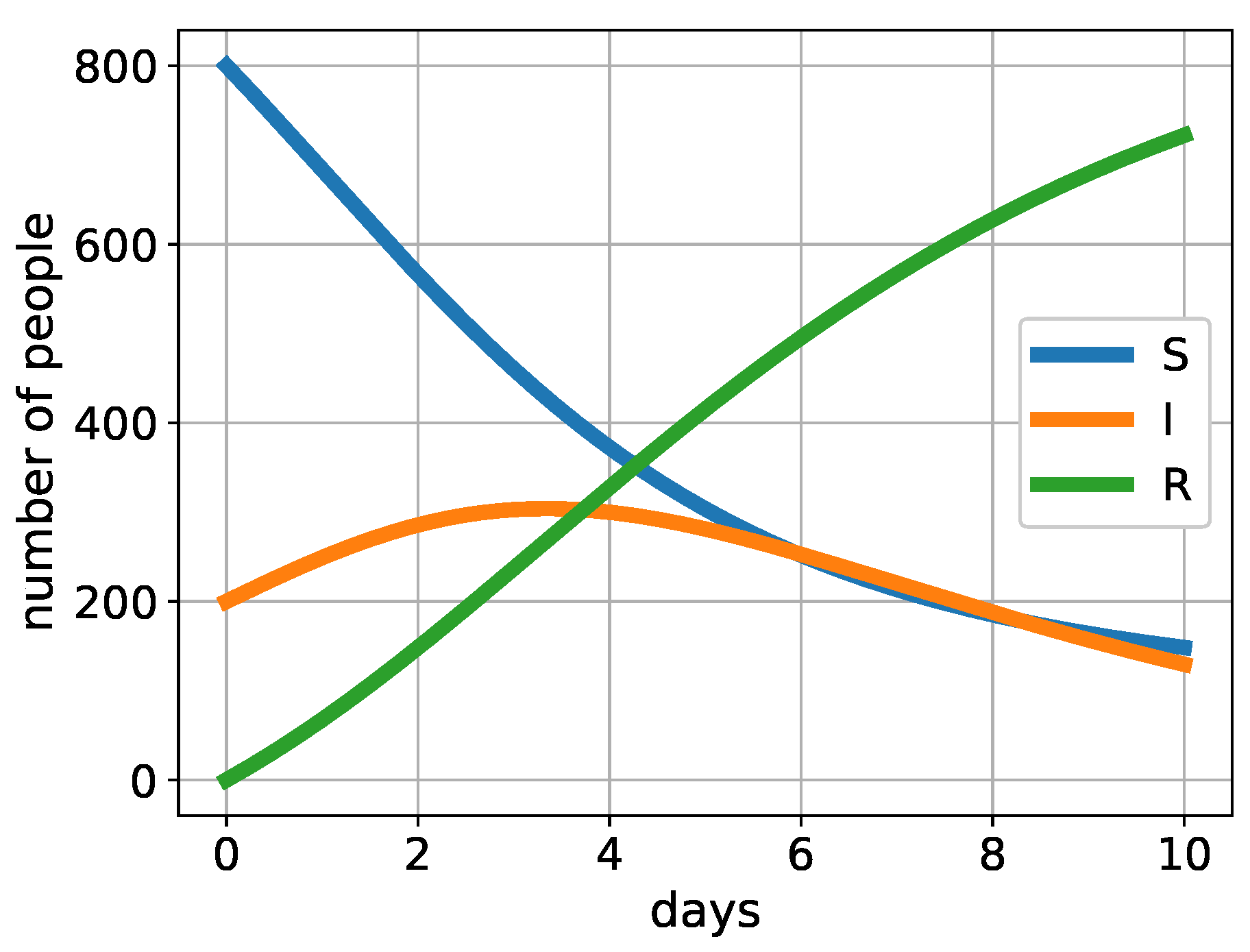
Here N is the population size. These parameters describe a single outbreak of an epidemic over a period of

T = 10

days with dynamics visually displayed in Figure 2.

For the inverse SIR MF problem, the values of the

β

and

γ

parameters were reconstructed only based on 10 daily measurements of the infected part of the population, that is, in the target function (16) we have the measurements

\vec{I} = (I_{0}, . ., I_{9})

and don’t have any of

R_{p}

Experiment №2

For the second experiment, we use the same data as in Experiment 1, but introduce a single noise into the known solutions

(I_{0}, . . ., I_{9})

that does not exceed 1 or 5%. The noise value is generated the same for each day measurement and displays the systematic error of the observer.

Experiments №3,4

Experiments 3 and 4 repeat Experiments 1 and 2, differing only in that all 4 parameters are reconstructed:

\vec{θ} = (β, γ, a_{c}, b_{c})

Experiment №5

The fifth experiment is aimed at testing the performance of the algorithm on real data. As real data, the dynamic of spread of Covid-19 in Novosibirsk was chosen for the 150 days from 2021-04-13. The data collected in this city and some others can be found at the link https://covid19-modeling.ru/data. As in the previous experiment, the full set of parameters

\vec{θ} = (β, γ, a_{c}, b_{c})

was restored. For the target function (16) computation, the daily measurements of the number of infected people

\vec{I} = (I_{0}, . ., I_{149})

were used. The modeling was carried out for different time periods, which was called the window of modeling

(w)

. This means that the parameters are reconstructed using only data of w days and for the specified period. For the full 150-days period, gluing of the corresponding number of periods for w days was done. The comparison of errors of modeling is provided for several values of w.

Experiment №6

And the last experiment repeats Experiment 5, but here for the parameters reconstruction the daily measurements of the infected and recovered parts of the population were used. That is, in the target function (16) we have the measurements

\vec{I} = (I_{0}, . ., I_{149})

and

\vec{R} = (R_{0}, . ., R_{149})

4. Results

This section presents the results of computational experiments described above.

Experiment №1

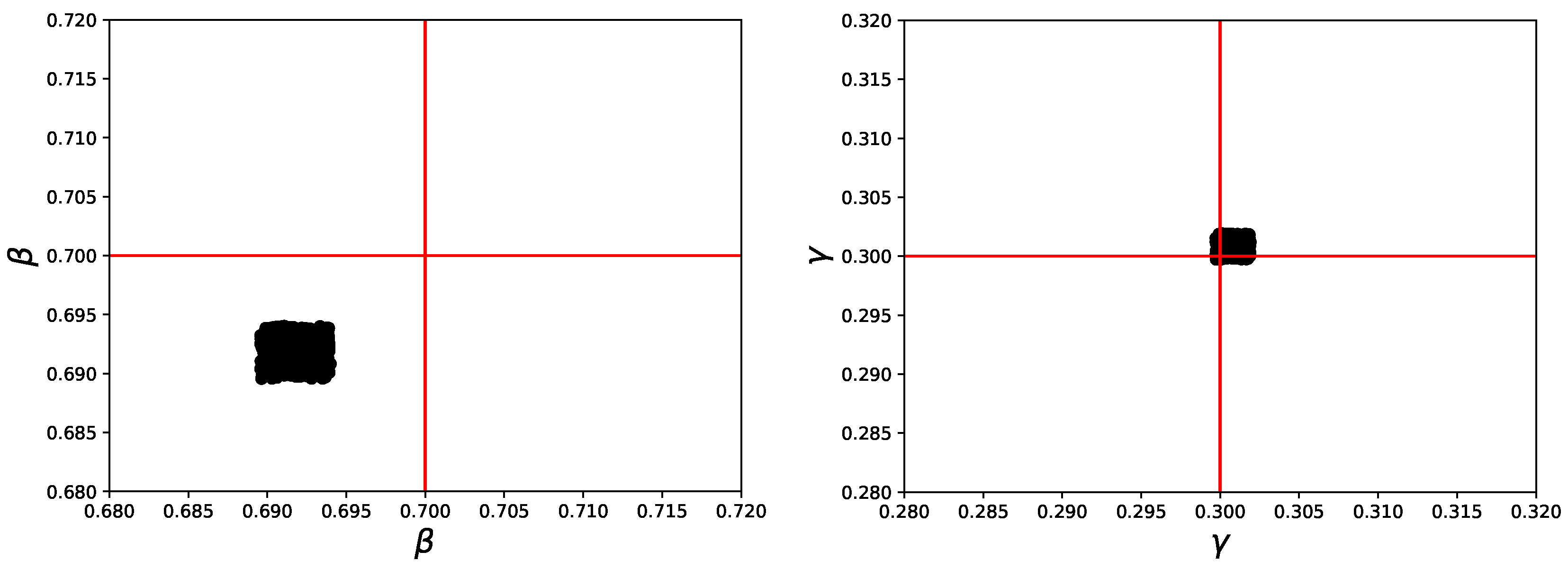
For the simple Experiment №1 which was aimed at recovering the main epidemiological parameters

β

γ

from synthetic data without any noise, the recovered parameters are

{0.69179788, 0.30081996}

versus the true one equaled

{0.7, 0.3}

. The initial values of

β, γ

for the optimization process were chosen equaled

{0.5, 0.5}

. Relative errors of recover are

1.2 %

and

0.3 %

. The 44 iterations of the algorithm, described in Section 3.2, were required.

Experiment №2

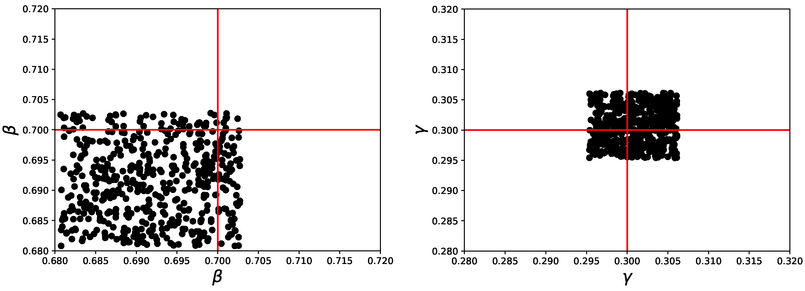
For the second experiment where the noise in measurements was put on the thousand of similar optimization problems with different generated value of noise were solved. The result of this is presented in Figure 3 and Figure 4 for noises the values of which don’t exceed 1% and 5%.

Here and after, metrics

r m s e

and

m a e

are used for estimating the results of computational experiments. The metrics are explained below.

r m s e = \sqrt{\frac{1}{M} \sum_{k} {(y - y_{k})}^{2}},

r a e = \frac{100}{M} \sum_{k} \frac{| y - y_{k} |}{| y |},

where y is true observation;

y_{k}

obtained value from kth experiment realization; M is number of realization. Thus,

r m s e

represents the root of the mean square error and

r a e

is relative absolute error.

So, for the Experiment №2, when introducing noise doesn’t exceed 1%:

r m s e

for

β

: 0.00830;

r a e

for

β

: 1.17%;

r m s e

for

γ

: 0.00103;

r a e

for

γ

: 0.29%.

When introducing noise doesn’t exceed 5%:

r m s e

for

β

is 0.01036;

r a e

for

β

is 1.22%;

r m s e

for

γ

is 0.00320;

r a e

for

γ

is 0.91%.

Experiment №3

The same pattern of computational results can be found for Experiments 3,4. The recovered parameters for Experiment №3 are

{0.69366844, 0.30132925 . 0.58164058, 0.00000000}

for

β, γ, a_{c}, b_{c}

. Thus, the relative absolute errors for

β

and

γ

amount to

0.90 %

and

0.44 %

correspondingly. The reconstructed parameter

b_{c}

equals zero because here as the true measurements the solution of SIR epidemiological problem (17) was used. This means that the optimal strategy

α

used in SIR MF model should be zero, and this is achieved when

b_{c} = 0

and any value of

a_{c}

Experiment №4

For the fourth experiment where the noise in measurements was put on the three hundred similar optimization problems with different generated value of noise were solved. The number of similar computations was reduced because of the long computation time of recovering 4 parameters. The visual representation of the distribution of reconstructed parameters

β

and

γ

are similar to that obtained from Experiment №2 (see Figure 3, Figure 4). The

r m s e

and

r a e

values for

β

and

γ

parameters are presented below.

When introducing noise doesn’t exceed 1%:

r m s e

for

β

: 0.00830;

r a e

for

β

: 1.17%;

r m s e

for

γ

: 0.00103;

r a e

for

γ

: 0.29%.

When introducing noise doesn’t exceed 5%:

r m s e

for

β

is 0.01036;

r a e

for

β

is 1.22%;

r m s e

for

γ

is 0.00320;

r a e

for

γ

is 0.91%.

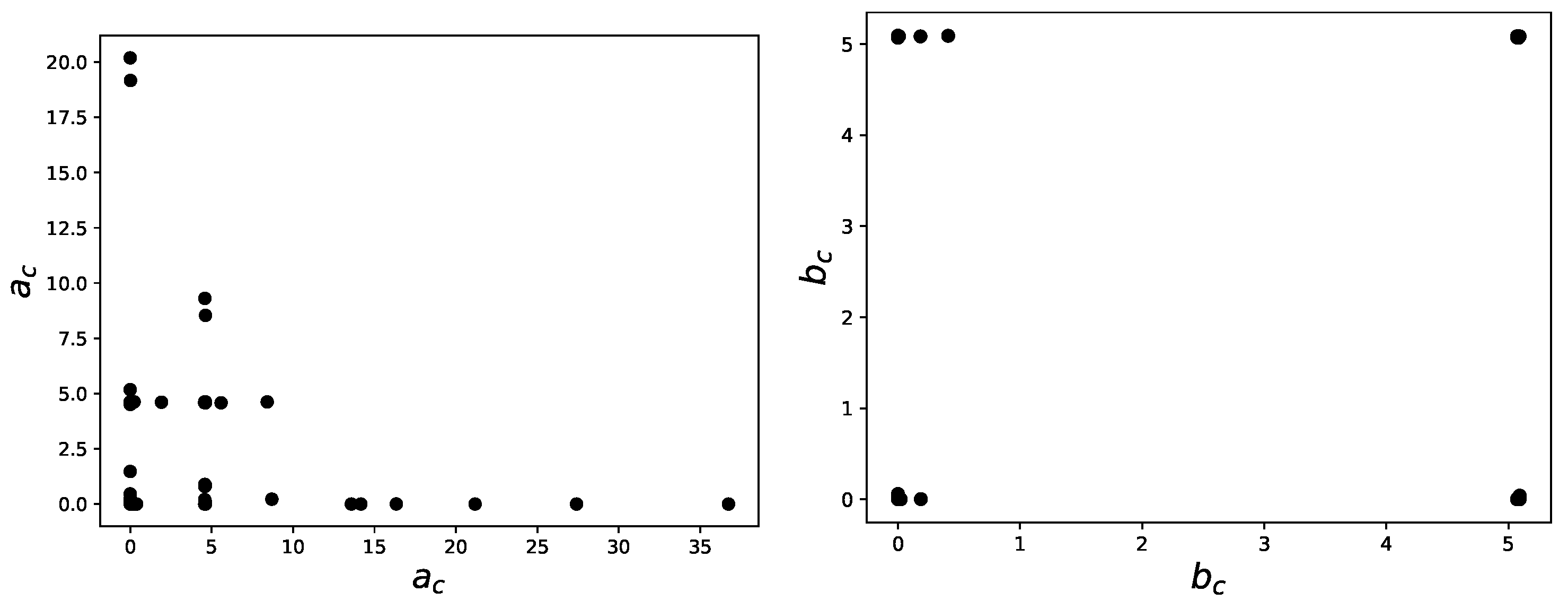
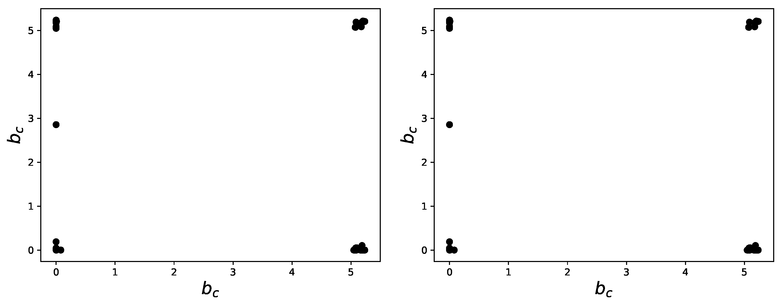
The reconstructed parameters

a_{c}

and

b_{c}

are presented in Figure 5 and Figure 6.

Experiments №5,6

The Figure 7 and Figure 8 show the result of computational experiments carried out on real data. In the case of Figure 7 the parameters were recovered using only measurements of the infected part (I group) of the population and after recovering they were used for direct modeling to compare the quality of approximation. For the result depicted in Figure 8 the same was done, but fore the recovering the measurements of infected and recovered parts (I and R groups) of the population were used. The figures depict the result for modeling window length (w) equaled 10 days.

The Table 1 includes the values of

r m s e

and

r a e

for several values of windows length w.

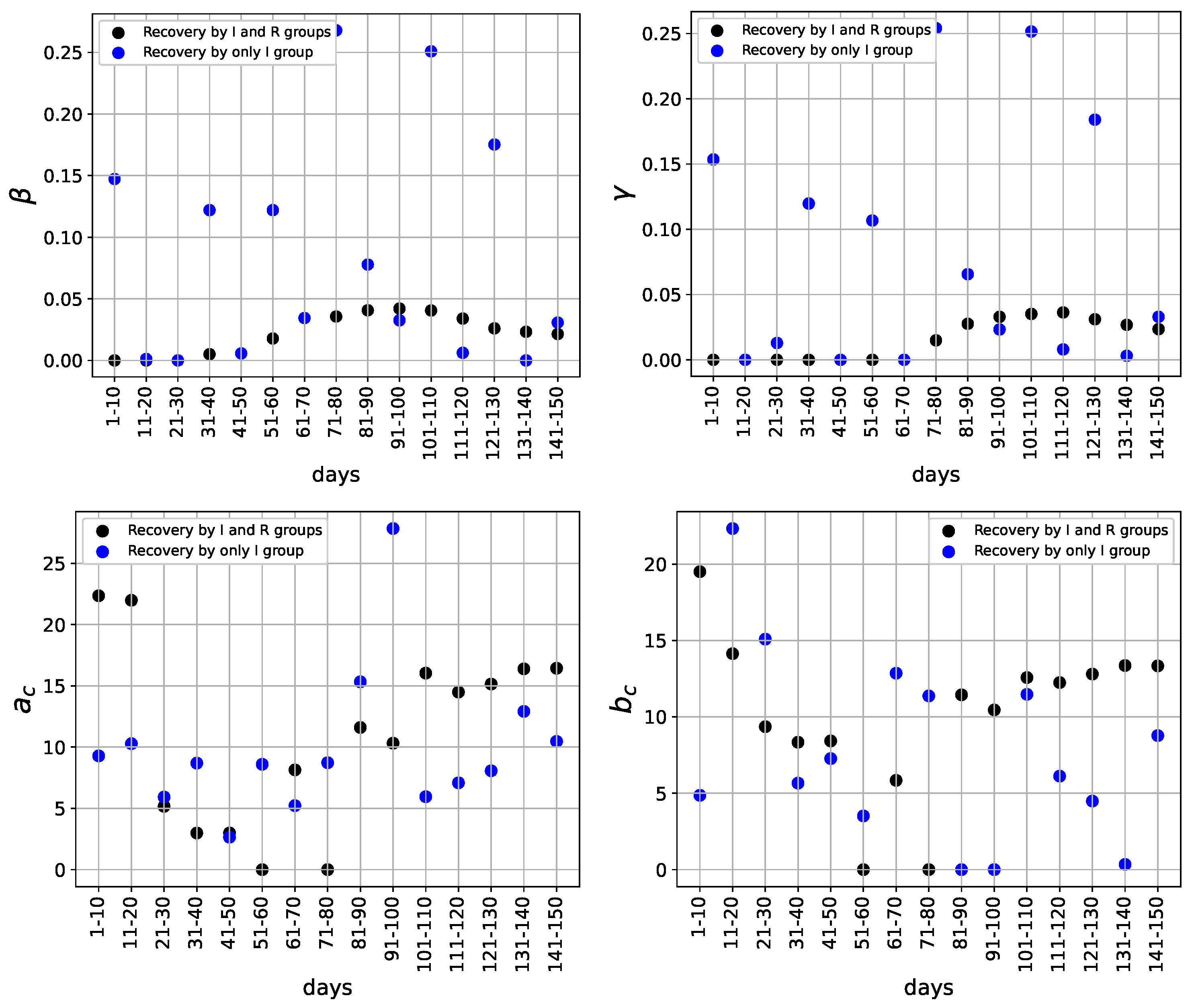
And the last picture Figure 9 shows the difference in determination of parameters

β, γ, a_{c}, b_{c}

when they were recovered using only the measurements of the infected part of population or both infected and recovered.

5. Discussion

This section is devoted to the analysis of the obtained results of computational experiments, discussion of current and future problems and ways of their solution.

As Section 2 of the work shows, the main difficulty in solving the inverse mean field problem lies in the restricted domain of existence and uniqueness of the solution of the direct problem. This makes the problem of reconstruction of the Hamiltonian of the system strongly ill-posed. However, the inverse problem for the mean mean field model describing the epidemiological process can be reduced to a coefficient problem. As the sensitivity analysis of the model, methodically carried out in [13], shows, the greatest influence on the modeling result is exerted by the choice of epidemiological parameters (for the SIR model, these are

β

and

γ

) and the growth rate of agent costs over time, that is, the choice of coefficients in the cost functional for a given behavior of the system.

The assertion that it is more important to restore the epidemiological parameters of the model relative to the general form of the Hamiltonian of the system is indirectly confirmed by the results of computational experiments 1-4. Here, the solution of the differential SIR model with known parameters was chosen as "exact measurements" and the obtained restored epidemiological parameters for the mean-field model were similar to those used. At the same time, the parameters

a_{c}

and

b_{c}

, describing the population, converged to values at which the solution of the mean-field model would coincide with the solution of the differential SIR model. Describe Figure 5,6 more detailed. In most cases, the value of

b_{c}

parameter was determined to be close to zero. This is an expected value because when

b_{c}

is equaled zero and

a_{c}

is any, the solution of SIR MF system coincides with the solution of SIR differential model. This also approves the variation in determination of

a_{c}

parameter. But in several cases, the value of

b_{c}

parameter is close to 5. This value was chosen as the initial value of parameters for the optimization problem. Thus, the simplex method used in the optimization algorithm determines that the initial value of the parameter is close to the optimal one. This indirectly confirms the hypothesis of a lower sensitivity of the model to the parameters describing the population, since when introducing an error into the "exact data", the greatest contribution to the system is made by the definition of the epidemiological parameters

β

and

γ

Note that here only the parameters before the costs of implementing the strategy (

a_{c}

) and the terminal conditions (

b_{c}

) were restored, while the growth rate of current costs remained unchanged, i.e. the function G in the cost functional was chosen to be reliably known. Such simplification is due to the fact that there are some relations on the growth rate of all three parts of the cost functional (the cost of implementing the strategy, current costs and terminal costs), which determine the area of existence of the solution to the direct problem. At present, these relations are unknown, but there is a hypothesis for their assessment based on the description of phase behavior of more complicated differential SIR models when describing a single outbreak. This is the future direction of studies of our research group.

Another problem related to the recovery of the mean field model parameters is the limited availability of measurements in each epidemiological group and the degree of confidence in such data. Statistical data of this kind are difficult to measure, since there is a large number of asymptotic patients and/or deaths from the consequences of infection, expressed in the form of exacerbation of chronic diseases. Thus, to recover the model parameters, it would be desirable to use only the part of the data in which there is strict confidence. Attempts to implement this in computational experiments with synthetic data, when the recovery was made only by measuring the number of infected people, gave an encouraging result. However, on real data (Experiments 5-6), the use of such an approach leads to non-uniqueness of the solution to the problem. An attempt to reduce the period for which the recovery is made also did not give results (see Table 1). Thus, to recover the model parameters on real data, there is a need for additional use of measurements in other epidemiological groups, at least partially, for example, the number of recovered people). This problem can be solved by using regularization, based on the work [20], where the regularization component is based on an assumption about the known values of the parameters. For example, the parameters being recovered over a certain period of time are not very different from those recovered over a previous period of time. This hypothesis also needs to be tested in future studies.

6. Conclusion

This work was devoted to a possible formulation of the mean field epidemiological problem. Section 2 proposes a formulation of the inverse problem coefficient, and provides its justification in the form of sensitivity analysis results. Section 3 describes the algorithm for solving such a problem and describes the computational experiments. Section 4 is devoted to the modeling results, and Section 5 is devoted to their discussion.

Research has shown that the presented formulation can be used to solve real epidemiological problems, but can be refined in two directions: regularization of the model to overcome the non-uniqueness of the solution to the problem on real data, and evaluation of the ratios of the components of the cost functional of the problem.

Funding

The work was performed according to the Government research assignment for Sobolev Institute of Mathematics SB RAS, project FWNF-2024-0002.

Data Availability Statement

Statistical data on Covid-19 incidence in Novosibirsk used for modeling are available at the link: https://covid19-modeling.ru/data . Data aggregated by epidemiological groups

(S, I, R

), used directly for the software implementation of the model are available at the link: https://disk.yandex.ru/d/jDVK3xsPwnNvPA.

Abbreviations

The following abbreviations are used in this manuscript:

SIS	Susceptible - Infected - Susceptible (differential model)
SIR	Susceptible - Infected - Recovered (differential model)
SIR TGC MF	SIR Mean Field model with Total Control for all epidemiological Groups
eFAST	Extended Fourier Amplitude Sensitivity Test

SIR MF	Susceptible - Infected - Recovered mean field (differential model)
N-M	Nelder-Mead (method)

References

Zanini, D.S.; Peixoto, E.M.; Andrade, J.M.D.; Tramonte, L. Practicing social isolation during a pandemic in Brazil: a description of psychosocial characteristics and traits of personality during covid-19 lockout. Frontiers in Sociology 2021, 6, 615232. [Google Scholar] [CrossRef] [PubMed]
Chen, J.; et al. pidemiological and economic impact of COVID-19 in the US. Journal Abbreviation 2021, 11, 20451. [Google Scholar]
Gao, X.; Yu, J. Public governance mechanism in the prevention and control of the COVID-19: information, decision- making and execution. Journal of Chinese Governance 2020, 2, 178–197. [Google Scholar] [CrossRef]
Capano, G. Policy design and state capacity in the COVID-19 emergency in Italy: if you are not prepared for the (un) expected, you can be only what you already are. Policy and Society 2020, 3, 326–344. [Google Scholar] [CrossRef] [PubMed]
La Torre, D.; Malik, T.; Marsiglio, S. Optimal control of prevention and treatment in a basic macroeco- nomic–epidemiological model. Mathematical Social Sciences 2020, 108, 100–108. [Google Scholar] [CrossRef]
Cho, S. Mean-field game analysis of SIR model with social distancing. Available online:https://arxiv.org/abs/2005.06758.
Roy, A.; Singh, Ch.; Narahari, Y. Recent advances in modeling and control of epidemics using a mean field approach 2023, 48, 207.
Petrakova, V.; Krivorotko, O. Mean field game for modeling of COVID-19 spread. Journal of Mathematical Analysis and Applications 2022, 514, 126271. [Google Scholar] [CrossRef] [PubMed]
Petrakova, V.; Krivorotko, O. Mean Field Optimal Control Problem for Predicting the Spread of Viral Infections. In Proceedings of 19th International Asian School-Seminar on Optimization Problems of Complex Systems (OPCS), Novosibirsk, Russia, 14-22 August 2023.
Ding, L.; Li, W.; Osher, S.; Yin, W. A mean field game inverse problem. Journal of Scientific Computing 2022, 92, 7. [Google Scholar] [CrossRef]
Chow, Y.T.; Fung, S.W.; Liu, S.; Nurbekyan, L.; Osher, S. A numerical algorithm for inverse problem from partial boundary measurement arising from mean field game problem. Inverse Problems 2022, 39, 014001. [Google Scholar] [CrossRef]
Liu, H.; Mou, C.; Zhang, S. Inverse problems for mean field games. Inverse Problems 2023, 39, 085003. [Google Scholar] [CrossRef]
Petrakova, V.; Krivorotko, O. Comparison of Two Mean-Field Approaches to Modeling An Epidemic Spread. JOTA 2024, submitted.
Lee, W.; Liu, S.; Tembine, H.; Li, W.; Osher, S. Controlling propagation of epidemics via mean-field control. SIAM Journal on Applied Mathematics 2021, 81, 190–207. [Google Scholar] [CrossRef]
Saltelli, A.; Tarantola, S.; Chan, K.S. A quantitative model-independent method for global sensitivity analysis of model output. Technometrics 1999, 41, 39–56. [Google Scholar] [CrossRef]
Nelder, J.A.; Mead, R. Simplex Method for Function Minimization. Computer Journal 1965, 7, 308–313. [Google Scholar] [CrossRef]
Lagarias, J.C.; Reeds, J.A.; Wright, M. H; Wright, P.E. Convergence Properties of the Nelder-Mead Simplex Method in Low Dimensions. SIAM Journal of Optimization 1998, 9, 112–147. [Google Scholar] [CrossRef]
Kolundzija, B.M.; Olcan, D.I. Antenna Optimization using Combination of Random and Nelder-Mead Simplex Algorithms. IEEE Antennas and Propagation Society 2003, 1, 185–188. [Google Scholar]
Chelouah, R.; Siarry, P. Genetic and Nelder-Mead Algorithms Hybridized for a More Accurate Global Optimization of Continuous Multiminima Functions. European Journal of Operational Research 2003, 148, 335–348. [Google Scholar] [CrossRef]
Shaydurov, V.; Petrakova, V. Three-parameter Regularization Algorithm for Pseudo-solution of Non-compatible Systems. Lobachevskii Journal of Mathematics 2024, 1, 328–335. [Google Scholar] [CrossRef]

Figure 1. Sensitivity indices for the SIR MF model (2)–(9) with a set of input parameters (13) for different simulation times:

T = 1, 3, 7, 15, 30, 90, 150

days

Figure 1. Sensitivity indices for the SIR MF model (2)–(9) with a set of input parameters (13) for different simulation times:

T = 1, 3, 7, 15, 30, 90, 150

days

Figure 2. Visual representation of the epidemic dynamics described by the SIR model (17) with parameters (18)

Figure 3. The values of recovered parameters

β

(left) and

γ

(right) for the 1000 carried out in similar Experiments №2 with uniform noise in data under 1%

Figure 3. The values of recovered parameters

β

(left) and

γ

(right) for the 1000 carried out in similar Experiments №2 with uniform noise in data under 1%

Figure 4. The values of recovered parameters

β

(left) and

γ

(right) for the 1000 carried out in similar Experiments №2 with uniform noise in data under 5%

Figure 4. The values of recovered parameters

β

(left) and

γ

(right) for the 1000 carried out in similar Experiments №2 with uniform noise in data under 5%

Figure 5. The values of recovered parameters

a_{c}

(left) and

b_{c}

(right) for the 300 carried out in similar Experiments №4 with uniform noise in data under 1%

Figure 5. The values of recovered parameters

a_{c}

(left) and

b_{c}

(right) for the 300 carried out in similar Experiments №4 with uniform noise in data under 1%

Figure 6. The values of recovered parameters

a_{c}

(left) and

b_{c}

(right) for the 300 carried out in similar Experiments №4 with uniform noise in data under 5%

Figure 6. The values of recovered parameters

a_{c}

(left) and

b_{c}

(right) for the 300 carried out in similar Experiments №4 with uniform noise in data under 5%

Figure 7. The result of direct modeling using SIR MF model in comparison with real data when the parameters of the model were reconstructed using the measurements of I group

Figure 8. The result of direct modeling using SIR MF model in comparison with real data when the parameters of the model were reconstructed using the measurements of I and R groups

Figure 9. The value of the reconstructed parameters in each 10-day simulation window relative to the real data

Table 1. Error values of the SIR MF model in comparison with real data depending on the chosen window length (w) for reconstruction of the model parameters

window length (w) (in days)	$m a e$ (in people)			$r a e$ (in percent)
window length (w) (in days)	S group	I group	R group	S group	I group	R group
Recovery by infected group (I) only
3	779.1	5.2	779.0	0.01	0.14	2.01
5	1052.0	9.0	1052.1	0.02	0.31	3.69
10	1124.1	19.5	1124.0	0.02	0.93	3.77
15	1198.5	21.6	1198.2	0.03	1.00	5.15
Recovery by infected and removed groups ( $I, R$ )
3	72.9	36.8	54.9	0.00	1.11	0.21
5	110.7	50.7	79.8	0.00	2.07	0.33
10	89.8	28.3	79.5	0.00	1.49	0.33
15	336.4	147.1	298.8	0.01	5.51	1.15

Disclaimer/Publisher’s Note: The statements, opinions and data contained in all publications are solely those of the individual author(s) and contributor(s) and not of MDPI and/or the editor(s). MDPI and/or the editor(s) disclaim responsibility for any injury to people or property resulting from any ideas, methods, instructions or products referred to in the content.

© 2024 by the authors. Licensee MDPI, Basel, Switzerland. This article is an open access article distributed under the terms and conditions of the Creative Commons Attribution (CC BY) license (http://creativecommons.org/licenses/by/4.0/).

Copyright: This open access article is published under a Creative Commons CC BY 4.0 license, which permit the free download, distribution, and reuse, provided that the author and preprint are cited in any reuse.

MDPI Initiatives

Important Links

Choose an area of interest and we will send you notifications of new preprints at your preferred frequency.

Disclaimer

Inverse Coefficient Problem for Epidemiological Mean Field Formulation

Abstract

1. Introduction

2. Mathematical Formulation

2.1. Direct Problem

2.2. Inverse Problem Formulation

3. Materials and Methods

3.1. Nelder-Mead Optimiaztion Method

3.2. The Algorithm for the Solution of the Coefficient Inverse SIR MF Problem

3.3. The description of computational experiments

4. Results

5. Discussion

6. Conclusion

Funding

Data Availability Statement

Abbreviations

References

MDPI Initiatives

Important Links

Subscribe