1. Introduction
Hemodynamics refers to the study of the movement and forces involved in the circulation of blood. The circulatory system is regulated by autoregulatory mechanisms of homeostasis, similar to how control systems regulate hydraulic circuits. The hemodynamic response constantly monitors and adapts to the situations within the body and its surroundings. Hemodynamics is the study of the physical principles that control the movement of blood within the blood arteries. Blood circulation facilitates the conveyance of nutrients, hormones, metabolic waste products, oxygen, and carbon dioxide throughout the body to sustain cellular metabolism, regulate the pH, osmotic pressure, and temperature of the entire body, and offer defense against microbial and mechanical damage. The heart serves as the primary propeller of the circulatory system, propelling blood through the body via rhythmic contractions and relaxations. The cardiac output (C.O.) refers to the volume of blood that is pumped out of the heart per minute, typically measured in liters per minute (L/min) [
1,
2].
The heart pumps blood into the aorta, which is the body’s most significant artery. Subsequently, it undergoes a process of branching into progressively narrower arteries, then into arterioles, and ultimately into capillaries, where the exchange of oxygen takes place. The capillaries are interconnected with venules, and subsequently, the blood is transported back through the intricate system of veins to the venae cavae, ultimately reaching the right heart. The micro-circulation, which includes the arterioles, capillaries, and venules, makes up the majority of the circulatory system and is where the exchange of oxygen, glucose, and enzyme substrates occurs between the cells. The venous system transports the blood lacking oxygen back to the right side of the heart, from whence it is propelled into the lungs to acquire oxygen. At the same time, carbon dioxide and other gaseous waste products are exchanged and released during the process of breathing. Subsequently, the blood is sent back to the left side of the heart, initiating the cycle once more [
3,
4,
5].
In a typical circulatory system, the amount of blood that flows back to the heart per minute is about equivalent to the amount that is expelled per minute (known as the cardiac output). The total cross-sectional area of that level essentially governs the velocity of blood flow at each level of the circulatory system.
There are two ways used to determine cardiac output. The Fick equation can be utilized as follows: C O = V O2 / (C a − C v) where V̇O2, oxygen consumption in mL of pure gaseous oxygen per minute, C.O. = Cardiac Output, Ca = Oxygen content of arterial blood, Cv = Oxygen content of mixed venous blood [
6,
7,
8].
Another thermodilution technique involves detecting the temperature variation resulting from the injection of a liquid into the proximal port of a Swan-Ganz catheter, which is then measured at the distal port.
The equation provided represents the mathematical expression for cardiac output.
The equation is represented as C O = S V × H R.
C.O. stands for cardiac output and is measured in liters per second (L/sec).
S.V. is the cardiac output, which is the amount of blood ejected from the heart during each beating, quantified in milliliters (ml) H.R. stands for heart rate, which is measured in beats per minute (bpm) [
9].
The typical cardiac output of a human at rest is 5-6 liters per minute. Not all blood that enters the left ventricle is expelled from the heart. The difference between the end-diastolic volume (E.D.V.) and the stroke volume is known as the end-systolic volume (ESV).
Blood, being a non-Newtonian fluid, is best analyzed using rheology rather than hydrodynamics. Hemodynamics cannot be explained by conventional hydrodynamics and fluid mechanics, which rely on the use of classical viscometers because blood vessels are not rigid tubes [
10].
The smoothness of blood arteries affects blood flow, leading to either turbulent (chaotic) or laminar (smooth) flow. The accumulation of fatty deposits on the artery walls diminishes smoothness.
The Reynolds number (N.R. or Re) is a parameter used to analyze the characteristics of fluid flow in a tube, specifically in the instance of blood flow in a vessel.
The mathematical expression representing this correlation, without considering units, is as follows:
The equation N R = ρ v L expresses the correlation among N, R, ρ, v, and L. In this context, the symbol ρ denotes the blood density.
The variable “v” denotes the mean speed of the blood.
The term “L” refers to the unique measurement of the vessel, specifically its diameter.
The symbol μ denotes the viscosity of blood [
11].
The Reynolds number exhibits a direct correlation with both the velocity and diameter of the tube. It should be noted that N.R. is directly related to both the average velocity and the diameter. Laminar fluid flow is characterized by steady flow motion when the Reynolds number is less than 2300, whereas a value of above 4000 indicates turbulent flow. The capillaries have a smaller radius and lower velocity compared to other vessels, which leads to a very low Reynolds number. As a result, the flow in the capillaries is laminar rather than turbulent [
12].
It is commonly measured in centimeters per second. The value is inversely proportional to the entire cross-sectional area of the blood artery. Furthermore, the variation occurs depending on the cross-sectional area due to the fact that, under normal circumstances, the blood flow exhibits laminar properties. Consequently, the velocity of blood flow is highest near the center of the vessel and lowest at the vessel wall. Typically, the average velocity is utilized. Various methods can be employed to quantify blood flow velocity, such as videocapillary microscopes with frame-to-frame analysis or laser Doppler anemometry. Arterial blood velocities are greater during systole compared to diastole. The pulsatility index (P.I.) is a metric utilized to quantify the disparity between the highest systolic velocity and the lowest diastolic velocity, divided by the average velocity during the heart cycle. This value decreases as the distance from the heart increases [
13].
Resistance is additionally impacted by variables such as the diameter and length of the blood artery, as well as the viscosity of the blood.
At first, we employ a fluid-based methodology, as recommended by the Hagen-Poiseuille equation. The equation is as presented:
The change in pressure is eight microliters. Q represents the flow rate, π represents the mathematical constant pi, and r4 represents the fourth power of the radius. ∆P represents the pressure drop or pressure gradient; μ: the measure of a fluid’s resistance to flow, commonly known as viscosity. The variable “l” represents the length of the tube. For vessels that have infinitely long lengths, the variable “l” is substituted with the diameter of the vessel. The variable “r” represents the radius of the vessel.
According to Thurston, a second approach, based on experimental measurements of blood flows, provides a more realistic understanding of vascular resistance. This method suggests that there is a layer of plasma release-celling surrounding a blocked flow at the walls. The fluid layer in actual blood flow is characterized by a varying viscosity η(δ), where δ represents the distance from the vessel center. It is important to note that these surrounding layers do not intersect at the vessel center. Alternatively, there is the phenomenon of blocked flow, characterized by its high viscosity due to the presence of a dense concentration of red blood cells (R.B.C.s). Thurston constructed this layer to quantify the resistance to blood flow by incorporating the viscosity η(δ) and thickness δ of the wall layer [
14,
15,
16].
The blood resistance law, represented by the symbol R, is modified to align with the blood flow profile.
The equation is given by R = c L η(δ) (π δ r3), where R represents the resistance to blood flow.
c represents the constant coefficient of flow.
L represents the measurement of the vessel’s length.
The symbol η(δ) represents the viscosity of blood in the wall plasma release-cell layers.
The variable “r” represents the radius of the blood vessel.
δ represents the distance within the plasma release-cell layer.
The resistance of blood is influenced by factors such as blood viscosity, the flow of blood through the vessel (either blocked flow or sheath flow), and the size of the vessels. Under the assumption of steady, laminar flow within the blood vessel, its behavior closely resembles that of a pipe. The pressure drop or gradient, denoted as Δp, can be calculated by subtracting the pressure at one end of the tube (p1) from the pressure at the other end (p2).
The more prominent arteries, which are visible to the naked eye, serve as conduits with minimal vascular resistance (assuming no significant atherosclerotic alterations). They exhibit rapid flow rates and produce negligible decreases in pressure. The smaller arteries and arterioles exhibit more excellent resistance, resulting in a significant reduction in blood pressure from the large arteries to the capillaries in the circulatory system [
17,
18].
Illustration depicting the mechanism by which vascular constriction, or vasoconstriction, leads to an elevation in blood pressure.
Arterioles have lower blood pressure compared to the major arteries. This phenomenon occurs as a result of bifurcations, which lead to a decrease in pressure. As the number of bifurcations increases, the total cross-sectional area also increases, resulting in a decrease in pressure over the surface. No evidence supports the reason for the largest pressure decrease in the arterioles, and citation is required. The pressure drop across the arterioles can be calculated by multiplying the flow rate by the resistance: ∆P = Q × resistance. The significant resistance reported in the arterioles, which predominantly affects the ∆P (pressure difference), is due to their lower radius of approximately 30 μm. As the radius of a tube decreases, the resistance to fluid flow increases [
19].
The capillaries are located just after the arterioles. Based on the observed logic in the arterioles, we anticipate that the blood pressure in the capillaries will be lower than that is applied, as pressure is defined as the force per unit area (P = F/A). Despite the small size of the capillary radii, the capillary network possesses the most extensive surface area among all the blood vessels in the body. The human vascular network is recognized for having the most comprehensive surface area, measuring 485 mm^2. As the overall cross-sectional area increases, both the mean velocity and the pressure decrease [
20].
Vasoconstrictors are substances that can constrict blood arteries, leading to an increase in blood pressure. Vasodilators, such as nitroglycerin, cause the dilation of blood arteries, leading to a reduction in arterial pressure.
An increase in blood viscosity leads to an elevation in arterial pressure. Specific medical diseases can alter the thickness or consistency of the blood. Anemia, characterized by a low concentration of red blood cells, decreases viscosity, while an increasing concentration of red blood cells increases viscosity. Previous beliefs said that aspirin and similar “blood thinner” medications lowered the thickness of blood, but research has revealed that its actual mechanism of action involves diminishing the blood’s propensity to form clots.
The formula used to calculate resistance is employed to determine the systemic vascular resistance (S.V.R.) [
21].
The formula for R is the change in pressure divided by the flow.
This can be translated as “Support Vector Regression” (S.V.R.).
The formula for calculating S V R is obtained by subtracting the constant variable P from the product of M A and P and then dividing the result by the constant variable O.
The abbreviation S.V.R. stands for systemic vascular resistance, which is measured in millimeters of mercury per liter per minute.
M.A.P. refers to the mean artery pressure, which is measured in millimeters of mercury (mmHg).
CVP is an acronym for central venous pressure, which is quantified in millimeters of mercury (mmHg).
C.O. stands for cardiac output, which is measured in liters per minute (L/min). The number 27 is enclosed in square brackets.
To convert this into Wood units, multiply the answer by 80.
The typical range for systemic vascular resistance is 900 to 1440 dynes/sec/cm−5.
The blood pressure at any given position is determined by the tension applied to the wall of the blood artery, as explained by the Young-Laplace equation. This equation assumes that the vessel wall’s thickness is insignificant compared to the lumen’s diameter.
The equation σ θ = P r t represents the relationship between the stress (σ θ) in a cylinder, the blood pressure (P), the wall thickness (t), and the inside radius (r) of the cylinder.
σ θ represents the stress exerted on a cylinder, sometimes referred to as “hoop stress.”
In order for the thin-walled assumption to be true, the vessel’s wall thickness should not exceed around one-tenth (also referred to as one-twentieth) of its radius.
The cylinder stress is the mean force applied in a circumferential direction (perpendicular to both the axis and radius of the object) on the cylinder wall. It can be defined as:
The equation for shear stress (σ) is equal to the applied force (F) multiplied by the distance (l) and divided by the cross-sectional area (θ).
Where: F represents the circumferential force applied to a section of the cylinder wall that has two lengths as its sides:
t represents the radial dimension of the cylinder
The variable “l” represents the axial length of the cylinder [
22,
23].
When a material is subjected to force, it undergoes deformation or displacement. The force required to deform a material, such as causing a fluid to flow, increases in proportion to the size of the material’s surface area. Therefore, the magnitude of this force (F) is directly proportional to the area (A) of the surface portion. Hence, the quantity (F/A), denoting the force exerted on a given area, is referred to as stress. The wall shear stress associated with blood flow through an artery is determined by the size and geometry of the artery and can vary from 0.5 to 4 Pa.
The equation is written as σ = F/A.
Shear stress is responsible for regulating its strength and orientation within an acceptable range to avoid the development of atherosclerosis, blood clotting, excessive growth of smooth muscle, and death of endothelial cells under normal circumstances. At times, when there is a sudden rise in blood pressure, shear stress can reach greater levels. At the same time, the counterflow can potentially change the direction of stress depending on the hemodynamic conditions. Therefore, this situation can lead to the formation of atherosclerosis [
24].
Veins are commonly known as the “capacitance vessels” of the body since they hold about 70% of the body’s blood volume within the venous system. Veins have higher compliance than arteries, enabling them to stretch and tolerate changes in volume [
25,
26].
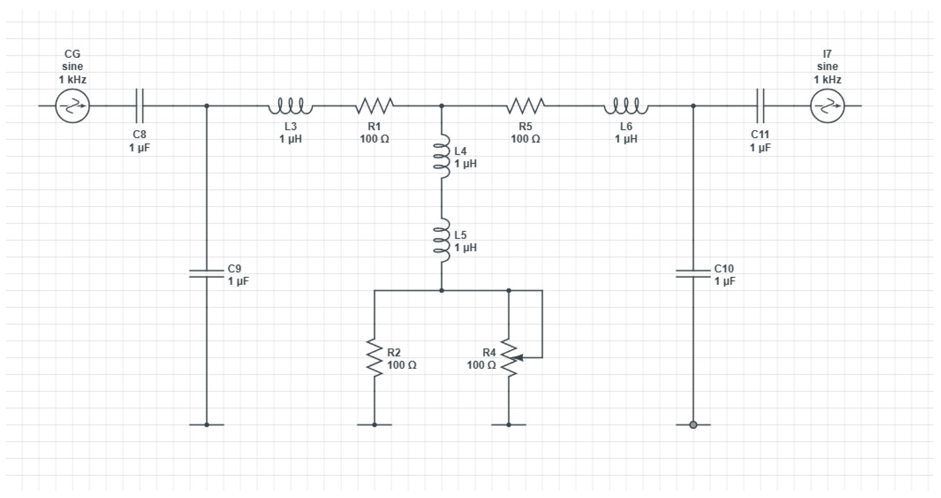
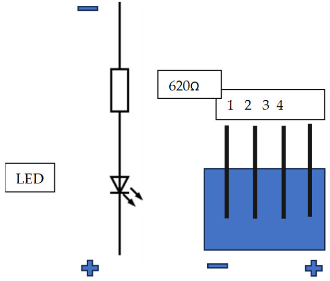
In this study, a P.C.B. device is proposed for studying arterial stenosis. The degree of stenosis is varied, leading to multiple readings.
3. Results
A continuous and variable voltage source was used to test the assembly. The test voltage was injected in point 1 of the primary electrical diagram of the assembly. The output voltage was collected from point 2 of the assembly and applied to the input of an oscilloscope. It is found that as the input voltage at point 1 increases, the value of the output voltage measured at point 2 increases accordingly for the interpretation of test results with a mathematical expression; a straight rectangular system is used in the plan. A flat Cartesian system includes two perpendicular axes: Ox - the axis of the values (of the variable (x)) and the oy axis - the axis of the function (Y). These axes are oriented in a perpendicular plane. On the axis of the value of the variable (x), respectively, the function (y) is positive, increasing starting from the holes (0,0). In the opposite sense, the values of the variable and the function decrease; they are positive until the origin and then become negative. The function (y) is repeated in cycles or periods.
The size for which the function takes values of the same meaning is called the half-period. A cycle (a period includes a positive half-period and a negative half-period. The function presents several periods in its domain of definition. The intersection of the two axes (ox) and (oy) is made at the coordinate points (0,0) called the origin, being perpendicular (make 90 degrees between them or right angles). The plane is divided into quadrants, numbered 1,2,3,4 (Table 1).
Table 1.
Domains of the y function in the fourth quadrans of a rectangular plane coordinates system.
Table 1.
Domains of the y function in the fourth quadrans of a rectangular plane coordinates system.
| Domain |
1 |
2 |
3 |
4 |
| Variable x |
+ |
- |
- |
+ |
| Function y |
+ |
+ |
- |
- |
| Interval |
0-π/2 |
π/2-π |
π-3π/2 |
3π/2-2π |
A practical example shows the sine function. A cycle (a period) extends over the interval (0.2π) on the Ox axis. On the interval (0, π), the function has positive values. This interval is a half-period. The interval (π, 2π) is the second half-period of the function. In the first half-period, the function is in the 1st quadrant, and in the 2nd half-period, the function is in the 4th quadrant. In test 5, there is a cut in the signal that is slightly pronounced so that it can be distinguished for the function with values close to the origin, such that the shape of the signal is convex. The usual porcine shape of the semen is easily highlighted.
Then, there is a sudden increase in the function, which stands out in the graph as the rectangular signal determined by a pronounced cut (interval A-B). In the negative area (interval B-C) , the signal is close to the rectangle-shaped shape, where the cut is made at a higher amplitude than in the positive part. The images obtained on the oscilloscope highlight the increase in the average voltage (Vavg) and the voltage between the peaks of the signals (Vpp) corresponding to one half-cycle of the signal recorded on the oscilloscope. The maximum amplitudes (peaks) are not visible on the oscilloscope, the signals being cut for both half-periods (positive located above the axis (ox) and negative situated in the lower part of the ox axis). The test image (40) includes the complete form of the signals, although VBpp has a relatively high value of 7.41V. The first three images, corresponding to test 1,14,33, are rectangular due to the “cutting” of the signals in amplitude. Image 33 indicates a slight deviation from the rectangular shape like this, as images 3 and 39 show a curvilinear graph; however, the voltage cuts in both semi-periods are visible. The stability of the signals on the oscilloscope screen is verified, proving the correct function of the assembly. The 50 Hz ester testing frequency is provided and indicated by the oscilloscope. A slight deviation of the frequency is evident in test 33, being 49.9 Hz (see supplemental material S2).
Table 2 shows the results of the experiments.
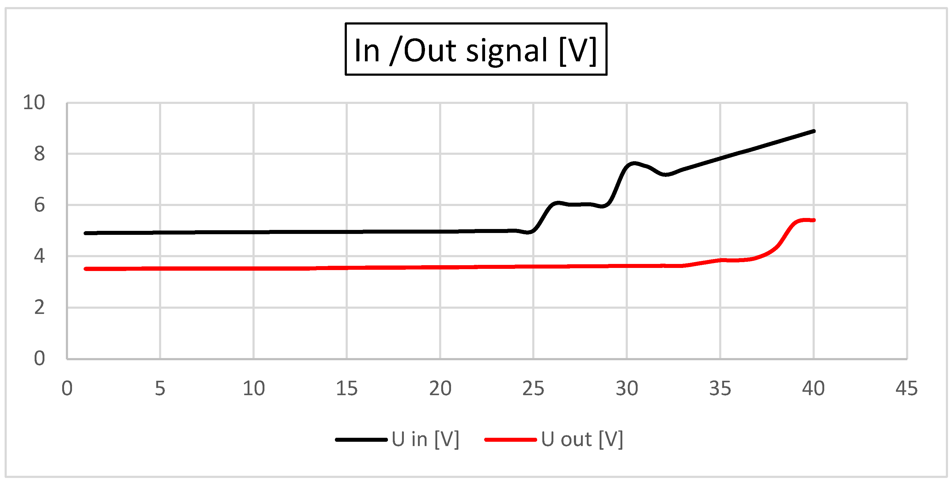
In
Figure 4, the signal input and output are shown [V]. As observed, the in and out signals remain constant, contrary to an increase in the system resistance (which mimics a stenosis). After the resistance [Ω] is increased by more than 50% of the base value, an increase in the in and out signals is observed.
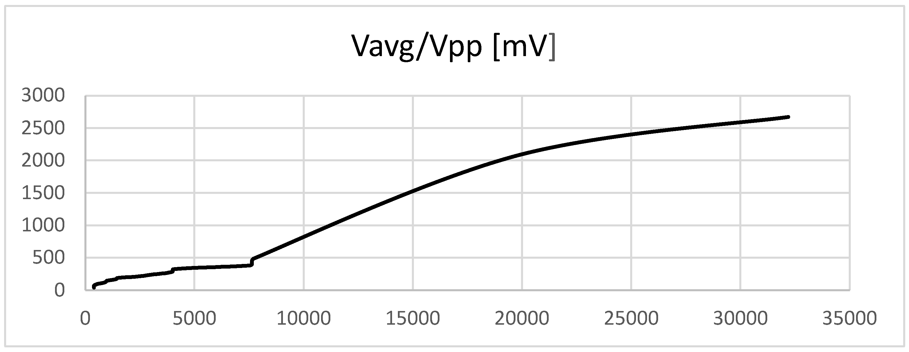
In
Figure 5, the average voltage versus the difference between the voltages is represented. Vagp and Vpp are very sensitive to changes in vascular resistance and increase with the increase in resistance (stenosis).
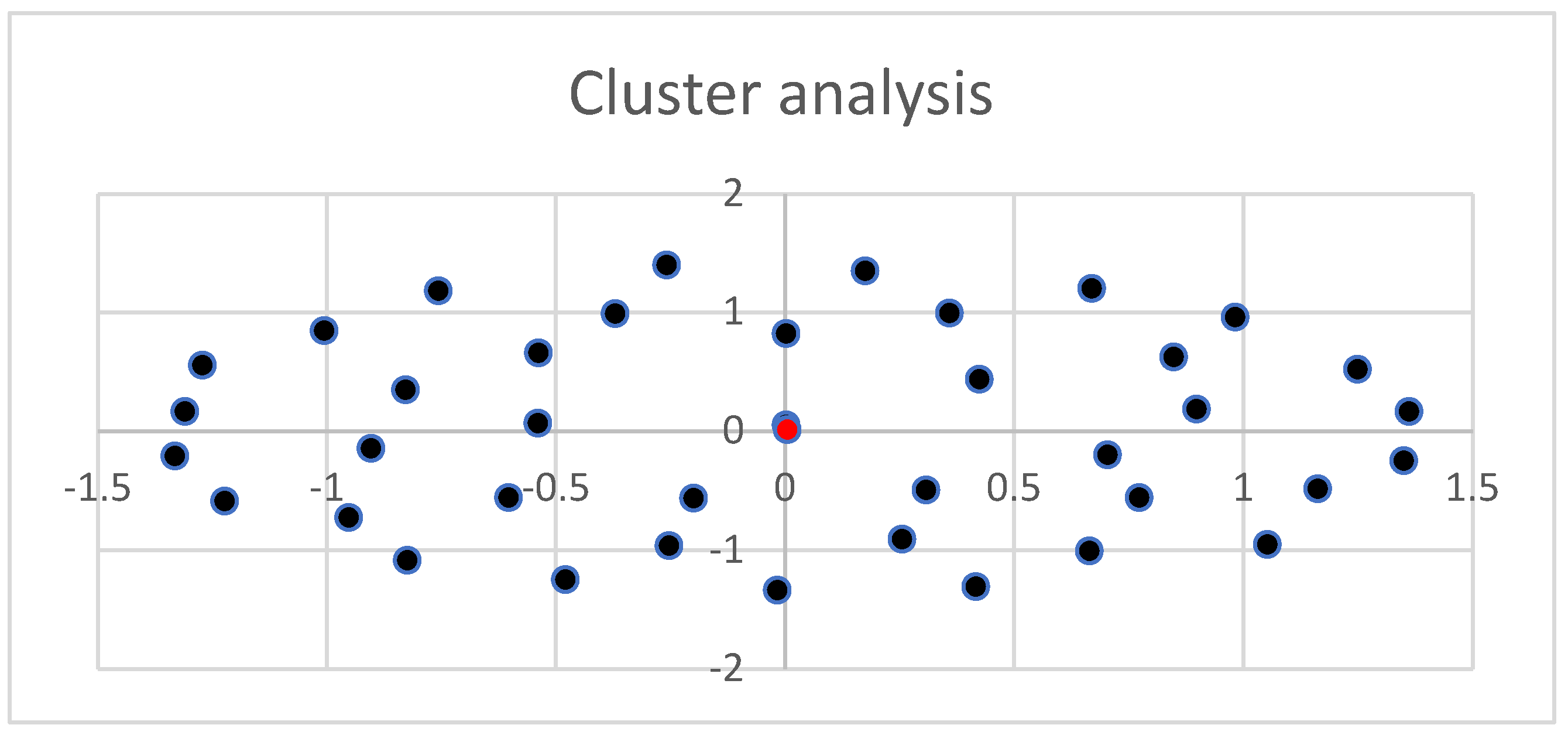
Figure 6 represents the cluster of all experimental observations. As observed, all values are part of the same cluster. The cluster is symmetric and distributed, suggesting that the data are average values and that there is an interconnection between them.
4. Discussion
Recent developments in computational performance and medical simulation technologies have markedly improved, especially in predictive diagnosis. This paper examines reduced-order models for blood flow simulation, hence serving as viable alternatives to 3D simulations in resource-constrained medical environments. This simplification leads to a reduction in spatial detail. Moreover, in hemodynamics research, user engagement with simulations might be crucial for pinpointing particular regions inside blood arteries that require thorough examination. For the application of CFD-based blood flow simulation in clinical practice, it is essential to achieve results in a timely manner. Conventional three-dimensional analyses necessitate significant processing resources, particularly when evaluating a diverse array of blood arteries, to ascertain local flow distribution. The considerable requirements for computer power and time make these studies unsuitable for swift clinical use. In contrast, economic blood flow simulations with reduced-order models have been created as diagnostic assistance instruments. Liang introduced a 1D–0D cardiovascular circulation model, wherein the 1D component calculates the deformation of the vessel wall and the corresponding pulse wave propagation by utilizing the surface integral over the cross-sectional area of the governing equation [
27,
28].
The 0D model simulates the mechanical characteristics of blood vessels by drawing parallels with electrical circuits. In literature, models are combined to simulate blood flow throughout the entire circulatory system. Those models represent major arteries as one-dimensional (1D) axisymmetric tubes, whereas peripheral blood vessels, veins, and the heart are depicted as zero-dimensional (0D) circuit components. The 0D elements are linked at both the commencement and conclusion of the 1D model, forming a closed loop. The 1D model governs the primary arteries, including the ascending aorta, and the circulatory systems of the upper body (Circle of Willis, external carotid arteries, and upper limbs) as well as the lower body, encompassing the abdominal region and, in this study, both lower and upper limbs. The one-dimensional elements connect to the zero-dimensional components at the terminal arteries and arterioles of each circulatory system. Veins converge in the heart’s right atrium and ventricle, with blood passing through pulmonary circulation before being ejected into the ascending aorta from the left atrium and ventricle, thereby re-entering the one-dimensional flow and initiating a new cardiac cycle [
29].
Blood circulation entails the propagation of pressure and flow waves throughout the vascular system. To balance computational efficiency and physical accuracy, one-dimensional (1D) network models have been employed to analyze pressure and flow waveforms in both normal and pathological states. This modeling methodology has been utilized for the systemic arterial system, the coronary network, and the brain vascular network. These one-dimensional network models comprise elements that locally delineate the relationship between pressure and flow. The relationship among pressure, area, and flow in blood vessels is described by one-dimensional wave propagation equations, specifically one-dimensional partial differential equations of mass and momentum, determined by integrating the Navier-Stokes equation across the cross-sectional area of the blood channel. As the caliber of vessels diminishes and their quantity grows towards the periphery, a threshold is achieved beyond which individual vessel modeling becomes unfeasible. At this juncture, the vasculature is abbreviated, and 0D lumped models, such as the Windkessel model or the structured tree model, elucidate the distal vasculature’s contribution to pressure and flow [
30].
Various complicated techniques exist to resolve the system of equations resulting from the 0D and 1D models and to simulate the propagation of pressure and flow waves through the vascular system. All numerical approaches for 1D wave propagation equations originate from the precise relationship among pressure, area, and flow or cross-sectional mean velocity. Initially, discrepancies among the numerical approaches emerge based on the selected state variables to be retained. The relationship between area and pressure, governed by a constitutive equation of the vessel wall, yields either a pressure-flow-area-velocity or a pressure-velocity formulation. A secondary source of discrepancies is the selection of spatial discretization for the equations. Techniques encompass finite difference and spectral/finite element methods. The outcome is a collection of ordinary differential equations requiring the temporal resolution of state variables. Thirdly, several techniques are employed to maintain the continuity of pressure and flow at vessel bifurcations and the junction between the vessels and the periphery. Methods encompass the weak coupling of 0D and 1D equations, the computation of Riemann invariants, or the incorporation of penalty equations [
31].
Considering 1 D models - in big arteries, blood pressure p (Pa), blood flow q (m³·s⁻¹), wall shear stress τw (Pa), and artery cross-sectional area A (m²) are interconnected through one-dimensional equations of mass and momentum. Neglecting leakage through the vessel wall and gravitational forces, the mass and momentum balance is expressed as follows (derivations can be found in Hughes and Lubliner and Van de Vosse and Stergiopulos: C.A.∂p∂t + ∂q∂z = 0, with C.A. = ∂A∂p, (1) ρA(∂q∂t + ∂∂z(δq²A)) + ∂p∂z = 2aτw(2) [
32,
33,
34].
In this (p, q, A) formulation, z (m) represents the coordinate along the vessel axis, a = √(A/π) (m) signifies the vessel radius, C A (m²·Pa⁻¹) indicates the vessel area-compliance, and ρ (kg·m⁻³) defines the blood density.
The wall shear stress τ w and the constant δ in (2) are determined by assuming a velocity profile. Multiple alternatives exist for selecting a velocity profile [
1]. This analysis assumes an approximate velocity profile. The wall shear stress is expressed as τw=−2η(1−ζc)aqA+a4(1−ζc)∂p∂z, where ζc=(max [0,1−2√α]).2. (3) where η (Pa·s) represents blood viscosity, ζ c denotes the fraction of cross-sectional area exhibiting inertia-dominated flow, and α=√2A0ρ/Tη is the Womersley number, which incorporates the time of the cardiac cycle T [s] and the vascular cross-sectional area A 0 = πa 0 2 at reference pressure p0. For approximate velocity profiles, the constant δ is defined as δ=2−2ζc(1−lnζc)(1−ζc)². (4) [
35,
36,
37]
The Poisson ratio μ, Young’s modulus E, and wall thickness h define the radius dependence of the area compliance. An expression for the pressure dependence of the cross-sectional area is derived by integrating the area compliance with pressure [
38].
The role of the peripheral vasculature at each artery endpoint is aggregated in a three-element Windkessel model. A singular differential equation is typically formulated that correlates pressure p and flow q at the entry of the Windkessel: ∂q/∂t = (1/Z)∂p/∂t + (p/ZC) - ((1 + Z.R.)q/ZC), (6) where Z denotes the characteristic impedance, R represents the peripheral resistance, and C signifies the peripheral compliance. However, the adoption of this equation implicitly presupposes that the venous exit pressure is zero. The model’s applicability is confined to that particular circumstance. A broader methodology involves constraining the Windkessel equations to those that correlate pressure differentials across the many components constituting the Windkessel model.
The role of the peripheral vasculature at each artery endpoint is aggregated in a three-element Windkessel model. A single differential equation is often formulated to connect pressure p and flow q at the Windkessel’s entrance.:
Let Z represent the characteristic impedance, R denotes the peripheral resistance, and C signifies the peripheral compliance. However, the adoption of this equation implicitly assumes that the venous exit pressure is null. The model’s applicability is confined to that particular circumstance. A broader methodology involves constraining the Windkessel equations to those that correlate pressure differentials across the many components constituting the Windkessel model [
39,
40,
41,
42].
The wave propagation equations for vascular segments are often expressed in discrete form utilizing finite/spectral-element or finite-difference methods. These approaches have the drawback that bifurcations necessitate the formulation of supplementary coupling equations based on Riemann invariants or penalty functions. Moreover, the equations of the peripheral model are typically integrated by resolving a characteristic equation in conjunction with the wave propagation equations. The limitation of this method is that the characteristic equation must be accessible. In the 0D model proposed, the data are directly available, being a fast and reproducible method.
Furthermore, the results provided by the 0D model are modest compared to the 2D-3D hemodynamics models presented in the discussion section. For those models, parallel computing is required. The exact anatomy of the vessel is usually recorded; thus, there is a need for extensive medical imagistic exploration (C.T., R.M.N.) before the model can be computed and the results analyzed.
