1. Introduction
Euclidean distance, a fundamental concept in geometry, is the most intuitive measure of spatial separation between points. Its computation is a core mathematical operation across various disciplines, including linear algebra, optimization, data analysis, and machine learning [
1]. In many algorithms within these fields, Euclidean distance is one of the most frequently performed computational operations and often constitutes a primary bottleneck in large-scale optimization problems, as clustering, nearest-neighbor searches, or high-dimensional data applications [
2]. Consequently, optimizing basic operations like distance computations can lead to significant improvements in the overall performance of many distance-dependent algorithms. For instance, in large datasets or real-time processing applications, reducing the overhead of distance calculations can substantially improve the speed and scalability of algorithms like K-means clustering or K-nearest neighbors (KNN) [
3]. This requires a deep understanding of both the mathematical properties of Euclidean distance and the specific characteristics of the problem at hand.
To address these challenges, several optimization strategies can be employed to accelerate distance computations. In this article, we provide a comprehensive review and comparative analysis of various optimization approaches aimed at improving the efficiency of Euclidean distance computations. The primary goal of these approaches is to reduce the computational burden associated with large-scale distance calculations.
Given two points
and
in an
n-dimensional space, the Euclidean distance
between them is defined as:
where
and
are the coordinates of the points
and
in
n-dimensional space
;
and
are the
kth components of
and
, respectively; and
is the norm of the vector difference between
and
[
4].
The Euclidean distance
defines a metric space by satisfying key conditions such as non-negativity, identity of indiscernibles, symmetry, and the triangle inequality [
5]. These properties give
its metric space structure, allowing for precise mathematical analysis of geometric relationships in the data.
Euclidean distance is a fundamental metric for quantifying similarity and dissimilarity, playing a key role in tasks such as clustering, classification, decision making, location tracking, route planning, anomaly detection, bioinformatics, and optimization [
6].
Many machine learning algorithms, including K-Nearest Neighbors (KNN), K-Means, Hierarchical Clustering, Principal Component Analysis (PCA), Vector Quantization (VQ), Mean Shift, and DBSCAN, depend heavily on distance calculations [
7,
8].
Beyond machine learning, Euclidean distance is crucial in image processing for tasks like edge detection, object recognition, and image segmentation [
9], and in geographic information systems (GIS) for route planning [
10] and spatial analysis [
11]. It is also central to anomaly detection, identifying outliers based on their distance from a central cluster, particularly useful in fraud detection and network security [
12]. In optimization problems such as the Facility Location Problem (FLP), it minimizes total travel distance, ensuring efficient facility placement, which is especially important in logistics and supply chain management [
13,
14].
In bioinformatics, Euclidean distance is employed to compare genetic sequences and biological samples [
15], clustering similar gene expression patterns, identifying biomarkers, and mapping evolutionary relationships [
16]. In robotics path planning [
17], it helps robots navigate the shortest path while avoiding obstacles, essential for precision in automated manufacturing, autonomous vehicles, and robotic surgery [
18].
In Natural Language Processing (NLP), Euclidean distance measures similarity between high-dimensional word embeddings or document vectors. These pairwise distance matrices are frequently used in graph-based methods, such as community detection, to uncover semantic clusters and build ontologies [
19,
20].
In numerous algorithms that employ Euclidean distance calculations, such as K-means clustering or K-nearest neighbors (KNN), computing these distances represents a significant computational burden, especially as the size of the data and the dimensionality increase [
21]. Each computation involves measuring the straight-line distance between pairs of points in a multidimensional space, which can be computationally intensive due to the necessity of performing multiple arithmetic operations. Full Euclidean distance calculations involve expensive operations like squaring differences, summing them, and taking square roots. Moreover, these distance calculations are not just performed once; they are typically executed repeatedly across many iterations of an algorithm. For instance, in each iteration of K-means, distances from each point to every cluster center must be recalculated to reassign points to the nearest cluster [
22]. Similarly, in KNN, distances are computed to all training data points to find the nearest neighbors for classification or regression [
23]. This repetitive computation can exponentially increase the time complexity and processing load, particularly with large datasets, making optimization of these distance calculations a crucial aspect of improving the efficiency and scalability of such algorithms.
Optimizing the computation of Euclidean distances can markedly enhance the performance of a multitude of algorithms where it is a fundamental, repeatedly executed operation [
24]. This is particularly true for data-intensive applications in fields like machine learning, data mining, and computer vision, where used algorithms rely heavily on frequent distance calculations. By refining these calculations the overall computational demand decreases. This not only speeds up the algorithms but also reduces energy consumption and allows for processing larger datasets or achieving higher throughput in real-time applications [
25]. Such enhancements in efficiency are crucial for scaling systems to handle the growing volumes and complexities of data encountered in modern analytical tasks, thereby broadening their applicability and improving their utility in practical scenarios.
Understanding these fundamental challenges and strategies is essential for researchers and practitioners working with large-scale and high-dimensional datasets. Optimizing Euclidean distance computations is not merely a technical necessity but a foundational step towards enabling more advanced data analysis and machine learning tasks in the era of big data.
2. Key Euclidean Distance Properties for Computational Optimization
Here, we summarize the main mathematical properties of Euclidean distance and how they can be efficiently used for its computational optimization:
Symmetry: . In pairwise distance calculations, this property lets you compute each distance once and store it in a symmetric matrix, halving the number of computations [
26].
Non-Negativity: . It provides a basic validation check during distance computations, allowing the algorithm to terminate early or avoid further incorrect computations [
1].
Identity of Indiscernibles: . This allows skipping distance calculations for identical points and filling the main diagonal of pairwise distance matrices with zeros, reducing unnecessary operations [
1].
Triangle Inequality (Subadditivity): This property states that for any points
A,
B, and
C, the direct distance between
A and
C is less than or equal to the sum of the distances through an intermediate point
B, i.e.,
. Triangle Inequality is crucial for reducing unnecessary distance calculations in clustering and nearest-neighbor algorithms. For example, in nearest-neighbor search, if
and
are known, you can skip calculating
if the inequality shows it is not needed [
27]. This property also enables optimizations in hierarchical clustering [
28] and network-based applications by using intermediate distances to avoid redundant computations. In KD-trees, the triangle inequality helps prune unnecessary comparisons, speeding up the search process [
29].
Spatial Locality: Points closer in space have smaller Euclidean distances, while distant points have larger distances. This property enables partitioning techniques, like KD-trees or Ball Trees [
29,
30], to group nearby points, allowing computations to focus on local regions instead of the entire dataset.
Monotonicity of the Square Root Function: The square root function is monotonically increasing, meaning that if
, then
. Many distance-based algorithms (e.g., KNN and K-means) only need relative distances. Skipping the square root and using squared Euclidean distance reduces computational complexity while preserving the distance order [
1,
31].
Dimensional Independence: Euclidean distance calculations can be performed independently for each dimension. This allows for parallelization, where each dimension’s contribution is computed separately, speeding up computations on multi-core processors [
3].
-
Additivity of Independent Dimensions or Subspaces: In high-dimensional spaces, Euclidean distance is the sum of squared differences across dimensions. Low-variance or threshold-exceeding dimensions can be skipped, enabling early termination and reducing computation with minimal accuracy loss [
24].
Scaling: While positive homogeneity is a property of norms, a similar scaling behavior holds for Euclidean distance under scalar multiplication. Specifically, for a scalar
, the distance between two points scales as
. This reflects that the distance is scaled by the absolute value of the scalar. After re-scaling, you can utilize previously computed distances and apply the scaling factor, avoiding full recomputation [
1].
Convexity: The squared Euclidean distance
is a convex function of its inputs. This property is crucial for optimization, as many algorithms (e.g., gradient descent) leverage convexity to ensure efficient convergence to a global minimum with fewer iterations [
4]. While the squared Euclidean distance is convex with respect to one variable when the other is fixed, the overall optimization problem may still be non-convex.
Continuity: Euclidean distance is continuous, so small changes in point positions cause small changes in distance,
. This allows for distance approximations in real-time applications, enabling faster computations in dynamic environments by skipping exact recalculations [
29].
Invariance under Geometric Transformations: Euclidean distance remains unchanged under translations, rotations, or reflections. For any transformation
T,
, enabling optimization by skipping distance recomputation, improving performance in graphics and simulations [
1].
Minkowski Special Case: Since Euclidean distance is a special case of the Minkowski distance with
, other Minkowski norms, such as the
-norm (
) and
-norm (
), provide upper or lower bounds. These bounds can be used for fast filtering: if an estimate using a simpler norm is already too large, further exact calculations can be skipped, improving performance [
1].
Sparsity Robustness: Euclidean distance computations in sparse vector spaces can be significantly optimized by only computing distances on non-zero dimensions. This property is particularly useful in large-scale machine learning tasks involving high-dimensional but sparse datasets, as it reduces the number of operations [
32].
Euclidean distance forms a metric space due to its properties (symmetry, triangle inequality, non-negativity, and identity of indiscernibles), enabling optimized search algorithms such as range queries, nearest neighbor searches, and clustering by reducing redundant calculations.
3. Key Approaches for Optimizing Euclidean Distance Computation
This section provides an overview of the main approaches for optimizing Euclidean distance calculations to accelerate the process. These approaches can generally be categorized into algorithm-specific methods, low-level optimizations, and hardware acceleration techniques. Additionally, hybrid approaches, which combine these methods, often yield the best results.
3.1. Algorithm-Specific Approaches
Algorithm-specific approaches for optimizing Euclidean distance computation focus on modifying or designing algorithms to reduce the number of required distance calculations by leveraging the mathematical properties of Euclidean distance, thereby minimizing computational overhead while preserving accuracy in distance measurements [
33].
Squared Euclidean Distance
One of the primary methods for reducing the computational load of Euclidean distance calculations involves algorithmic optimizations that minimize the number of required operations. A straightforward optimization is to eliminate the computationally expensive square root operation when only relative distances between points are needed, as in K-nearest neighbors (KNN) or K-means clustering. Since the square root is a monotonically increasing function, the ordering of distances remains unchanged, allowing the use of squared Euclidean distance instead [
1]. This simplification is particularly beneficial for large datasets, as square root operations are more computationally intensive than basic arithmetic. Additionally, using squared Euclidean distance not only enhances computational efficiency in the K-means algorithm but also improves its mathematical tractability [
31].
For instance, in clustering techniques, the Euclidean distance is integral to solving the Minimum Sum-of-Squares Clustering (MSSC) problem [
22], where the objective is to partition a set of data points
into
K clusters
such that the sum of the squared Euclidean distances between each point and the centroid of its assigned cluster is minimized, that is by minimizing the total within-cluster variance:
where
denotes the squared Euclidean distance between the data point
and the centroid
of cluster
. From a computational perspective, the squared Euclidean distance
is computed by simply eliminating the computationally expensive square root operation from the standard Euclidean distance and can be considered as one of the possible optimization approaches:
Given that the square root function is monotonically increasing, minimizing the squared Euclidean distance
is mathematically equivalent to minimizing the Euclidean distance
:
This equivalence ensures that the cluster assignments obtained by minimizing the squared distance are identical to those obtained by minimizing the unsquared distance. This elimination simplifies computations, especially for large datasets, as square root operations are more computationally intensive than basic arithmetic operations.
The squared Euclidean distance
is a quadratic function, which is convex with respect to each data point
individually when the centroid
is fixed. However, the overall objective function (
2) in the MSSC algorithms is not convex with respect to both the cluster assignments and centroids simultaneously. Therefore, the K-means algorithm can converge to a local minimum, which is not necessarily the global minimum [
34]. To find solutions closer to the global minimum, more sophisticated MSSC algorithms are typically employed [
3].
Despite the non-convexity of the problem, the differentiability of the squared Euclidean distance allows for the straightforward derivation of update rules within the K-means algorithm. Specifically, the centroid
of a cluster
can be straightforward and efficiently computed as the mean of the data points within that cluster:
The K-means algorithm iteratively assigns each data point to the cluster with the nearest centroid , and then updates each centroid by calculating the mean of all data points assigned to that cluster, i.e., , iteratively minimizing the within-cluster variance until convergence.
A remarkable feature of the K-means algorithm is its ability to naturally and iteratively minimize the sum of squared Euclidean distances,
, making it particularly well-suited for large-scale clustering tasks. This natural minimization occurs through the algorithm’s intrinsic process of reducing the sum of squared distances between data points and their respective cluster centroids by alternating between assignment and update steps, ultimately leading to convergence without the need for external adjustments [
34].
By utilizing the squared Euclidean distance (
3), the K-means algorithm achieves computational efficiency and mathematical tractability, even though it may converge to a local minimum [
31]. This approach enables the algorithm to find meaningful cluster configurations in a computationally feasible manner, though it may not always guarantee the global optimum of the clustering objective. However, this disadvantage can be mitigated by using simple techniques like Multi-start K-means [
34] clustering, which helps to obtain near-optimal solutions.
Lower Bound Techniques
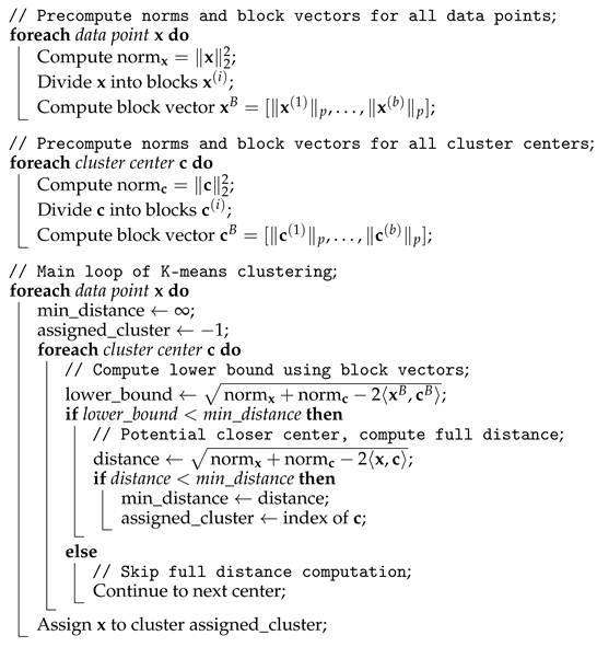
The block vector approximation [
2] allows the K-means algorithm to avoid unnecessary full distance calculations by providing a lower bound on the Euclidean distance between a point and a cluster center. This lower bound enables the algorithm to make early decisions about whether a cluster center can possibly be the closest center, thereby eliminating the need for a complete calculation of computationally expensive Euclidean distance in many cases.
Initially, to form the block vector representation, the given a high-dimensional data point
, it is subdivided into smaller sub-vectors, or
blocks, of fixed sizes along the dimensions:
where each
represents a subset of consecutive components of
. For each block, the
p-norm of the sub-vector is computed, resulting in a block vector
:
This process reduces the dimensionality of the original vector while retaining essential information about its structure. During the K-means algorithm, each point
is assigned to the closest cluster center. For a point
with a known closest center
, the lower bound on the distance to any other center
is computed using the block vectors. By using Hölder’s inequality, the inner product
is approximated by the inner product of the block vectors
. If the lower bound on the distance to
is greater than the actual distance to the current closest center
, i.e.,
then
cannot be the closest center, and the algorithm skips the full Euclidean distance calculation for
. Here the expression
refers to the squared Euclidean norm of the vector
. This results in significant computational savings, especially when there are many centers.
Algorithm 1 illustrates the snippet of K-means pseudocode leveraging lower bounds from block vector approximations to accelerate clustering.
|
Algorithm 1: Snippet of K-means pseudocode with Block Vectors optimization |
 |
The core computational saving comes from the fact that block vectors are much shorter than the original vectors, and the dot product of block vectors is much cheaper than a full Euclidean distance computation. Since can be precomputed for all x, they don’t need to be recomputed in every iteration. This mechanism works particularly well when there are a large number of clusters, or when the data is high-dimensional, as the savings in computation increase in such scenarios.
Triangle Inequality
The triangle inequality property [
1],
, can be used to prune unnecessary distance calculations. In certain cases, if a partial distance is already larger than a known threshold, further calculation can be skipped, as the result will not affect the outcome [
27].
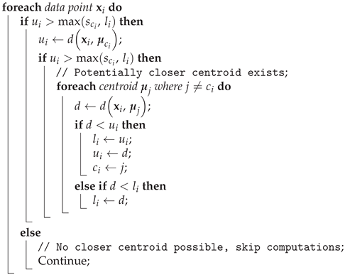
For example, Hamerly’s method [
35] for accelerating the K-means algorithm leverages the triangle inequality to significantly reduce the number of distance calculations required during clustering. In the naive K-means algorithm, the distance
between each data point
and every cluster centroid
is recalculated in each iteration, resulting in a computational complexity of
per iteration, where
m is the number of points and
k is the number of clusters. Hamerly’s method optimizes this process by maintaining upper bounds
and lower bounds
on the distances between each point
and its closest and second closest centroids, respectively. The algorithm also calculates a threshold
for each cluster, representing half the minimum distance between the centroid
and any other centroid:
. Using the Triangle Inequality, it can skip unnecessary distance calculations if the current bounds indicate that the point cannot be closer to another centroid than its current assignment. Mathematically, this is achieved by comparing the upper bound
to the maximum of
and
, and only recomputing distances when necessary. Algorithm 2 presents a pseudocode snippet that demonstrates how Hamerly’s method efficiently reduces distance computations in the K-means algorithm when recalculating distances between points and centroids. In the presented pseudocode,
denotes the index of the centroid (or cluster) currently assigned to data point
. This approach effectively reduces the number of Euclidean distance calculations, resulting in a more efficient algorithm that converges faster than the naive K-means while maintaining the same accuracy in clustering.
|
Algorithm 2: Snippet of K-means pseudocode with Triangle Inequality optimization |
 |
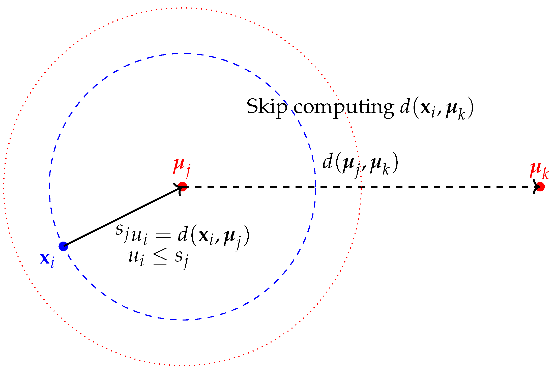
Figure 1 illustrates the positions of data points and centroids on a number line, highlighting the distances and thresholds used to apply the triangle inequality in skipping distance computations during K-means clustering. In this example, the data point
is closer to centroid
than to centroid
, and the upper bound
is less than the threshold
. This condition allows us to skip the computation of the distance
.
Recursive Distance Updating
Another widely-used method in data analysis that heavily relies on Euclidean distance computations is agglomerative hierarchical clustering [
28], which builds a hierarchy by repeatedly merging the closest clusters until all points form a single cluster. Starting with each point as its own cluster, the algorithm merges the pair with the smallest distance and recalculates the distances between the newly merged cluster and all remaining clusters. In its naive implementation, this requires recalculating distances from scratch after every merge, making it computationally expensive for large datasets, as the number of pairwise distance calculations increases quadratically.
Ward’s method, one of the most efficient techniques for agglomerative hierarchical clustering, is an example of how to minimize Euclidean distance recalculations when solving the Minimum Sum-of-Squares Clustering (MSSC) problem. Ward’s method efficiently minimizes within-cluster variance (
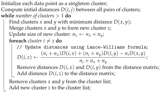
2) after merging clusters. It benefits from a recursive update mechanism known as the Lance–Williams formula, which optimizes the process of updating distances between the newly merged cluster and the remaining clusters. Instead of recalculating distances from scratch, the Lance–Williams formula updates the distances based on previously known distances and the sizes of the clusters involved in the merge. The Lance–Williams formula is:
Here, is the distance between cluster i and the newly formed cluster z (created by merging clusters x and y); , , and are the sizes of clusters i, x, and y, respectively; , , and are the pairwise squared Euclidean distances between these clusters.
Algorithm 3 presents pseudocode demonstrating how the Lance–Williams formula is used to efficiently update distances during agglomerative hierarchical clustering.
|
Algorithm 3: Hierarchical clustering algorithm using Lance-Williams formula for recursive distance updating |
 |
Using the Lance–Williams formula and the nearest-neighbor chain algorithm [
36], agglomerative hierarchical clustering achieves a time complexity of
, a significant improvement over the naive
approach.
Advanced Initialization
One effective strategy to reduce the computational burden in distance-intensive algorithms is to employ better initialization techniques, particularly in algorithms that rely on iterative local or global search [
34]. Many such algorithms, like K-means clustering, repeatedly compute distances as they iteratively refine their solutions. Poor initialization, such as random selection of initial centroids in K-means, can lead to significantly more iterations and, consequently, a higher number of distance calculations. By contrast, advanced initialization methods can result in fewer iterations and thus fewer distance computations.
In K-means, for example, the algorithm starts by randomly selecting K centroids and iteratively refines them by recalculating distances between data points and centroids in each iteration. With random initialization, the algorithm often converges slowly due to poor starting points, requiring many iterations to find optimal centroids. Each iteration involves distance computations, where n is the number of data points and K is the number of clusters. Therefore, reducing the number of iterations directly reduces the number of distance calculations.
Advanced initialization techniques, such as K-means++ [
37], provide a more strategic selection of initial centroids, leading to faster convergence. K-means++ initializes the centroids by probabilistically selecting data points that are farther apart, which ensures a better spread of centroids across the dataset. This reduces the number of iterations required for convergence compared to random initialization, ultimately reducing the number of Euclidean distance calculations performed during the algorithm.
An even more sophisticated initialization technique involves using the output of Ward’s method as the initial centroids for K-means. Ward’s method is aligns well with the objective of K-means [
36]. By first applying Ward’s method and then using its cluster centroids as the starting points for K-means, the algorithm often converges in far fewer iterations than with K-means++ or random initialization. This combination can significantly reduce the number of distance computations, as the initial centroids are already near optimal. Furthermore, alternating between different MSSC clustering algorithms, such as using Ward’s method followed by K-means (i.e., using Ward’s output as the input for K-means), can often improve the clustering outcome by further minimizing the objective function (
2) compared to running each algorithm in isolation, as the strengths of each method complement one another in refining the cluster assignments [
22].
Precomputing and Caching Distances
In certain scenarios, such as when working with static datasets, it is possible to precompute the pairwise Euclidean distances between all points and store them in a distance matrix, which is a key component in many machine learning and data analysis tasks [
26]. This precomputation, while expensive in terms of memory, allows for instant retrieval of distances during the optimization process, thereby eliminating the need for repeated calculations. Caching strategies can also be employed when the dataset is too large to store all pairwise distances, ensuring that frequently accessed distances are quickly available.
For a set of
m points
in
n-dimensional space, the precomputed Euclidean distance matrix
is an
symmetric matrix, leveraging the property
, where the entry
represents the Euclidean distance between points
and
[
32]. Mathematically,
is defined as:
In this formulation, the symmetry of the matrix is explicitly used by calculating only for and setting for . This approach allows for the computation of only half of the distance matrix—the elements below the main diagonal (the lower triangle), significantly reducing the number of distance calculations from to for a dataset with m points.
To save space by storing only the lower triangular part of a symmetric matrix
, its condensed (or compact) representation
can be used. The condensed matrix
is a vector containing the
elements of the lower triangular part of
, excluding the diagonal. The index
k in the condensed matrix
, corresponding to the element
in the full matrix
, is given by:
where
(assuming 0-based indexing). The condensed matrix
thus contains a total of
elements. To reconstruct the indices
in the full matrix
from the index
k in the condensed matrix
, the following formulas can be used:
where
denotes the ceiling function, and
denotes the floor function, which truncates the decimal part to return an integer value.
The bottleneck of the K-means algorithm is the repeated distance recalculations in each iteration. This is necessary because centroids are updated as the mean values of the assigned points, which are not actual data points. The K-means algorithm can be accelerated by using a precomputed Euclidean distance matrix
, where
, to avoid redundant computations. An optimized alternative is the K-medoids algorithm, which improves efficiency by leveraging the precomputed distance matrix and reducing the impact of outliers by using actual data points (medoids) as cluster centers [
38].
Unlike K-means, which computes distances to centroids, K-medoids assigns points to medoids based on precomputed distances from matrix
. The objective of K-medoids is to minimize the total dissimilarity between points and their medoids, defined as:
where
is the medoid, and
is the precomputed Euclidean distance. The algorithm iteratively refines the medoids by swapping them with non-medoid points and recalculating the total cost until convergence, making it especially beneficial for large datasets where recalculating distances is expensive.
In large datasets, there is a trade-off between computation time and memory usage when calculating Euclidean distances. Precomputing all pairwise distances in a matrix speeds up algorithms by avoiding redundant recalculations, but this approach demands substantial memory. Storing the full distance matrix for m points requires memory, which becomes impractical for large datasets. For example, with , it would need around 80 GB of memory. While manageable for small datasets, this approach is infeasible for larger ones. To reduce memory usage, a condensed matrix can be employed, leveraging the symmetry and zero diagonal , storing only the necessary elements.
Spatial Data Structures and Approximate Methods
The Euclidean distance is central in the K-nearest neighbors (KNN) algorithm, where it is employed to quantify the proximity between data points [
23]. Given a set of training data
where
represents the feature vectors and
denotes the corresponding class labels, the KNN algorithm classifies a new data point
by identifying the set
of the
K nearest neighbors, defined as:
The algorithm then assigns the class label
y to
based on the majority class among its nearest neighbors:
where
is the indicator function. Thus, the Euclidean distance serves as a crucial metric in determining the classification of data points based on the proximity of their neighbors within the feature space.
Nearest neighbor search is a common task in many machine learning algorithms [
6]. In nearest neighbor search the goal is to identify the closest point in a dataset
to a query point
. The naive approach involves computing the Euclidean distance from
to each point in the dataset, which has a time complexity of
. For large datasets and high-dimensional spaces, this approach can be prohibitively expensive.
Besides the use of precomputed pairwise distance matrices, one of the most effective strategies to accelerate nearest neighbor search is the use of spatial data structures such as KD-trees [
29] and Ball Trees [
30]. These structures enable a partitioning of the dataset into hierarchical regions, allowing the algorithm to discard large portions of the dataset that are unlikely to contain the nearest neighbor, thus reducing the number of distance computations.
Spatial data structures, such as KD-trees, exploit the Spatial Locality property of Euclidean distance by organizing data points in a way that nearby points are grouped together and distant points are separated. The Spatial Locality property implies that points closer in space have smaller Euclidean distances, while those farther apart have larger distances.
The KD-tree algorithm operates by recursively splitting the dataset into two halves along the median of one of the dimensions at each level of the tree [
29]. Given a query point
, the KD-tree can be traversed to rapidly exclude regions of the space that are farther from
than the currently identified nearest neighbor. While the KD-tree is efficient in low to moderate dimensions, its performance degrades in high-dimensional spaces due to the curse of dimensionality.
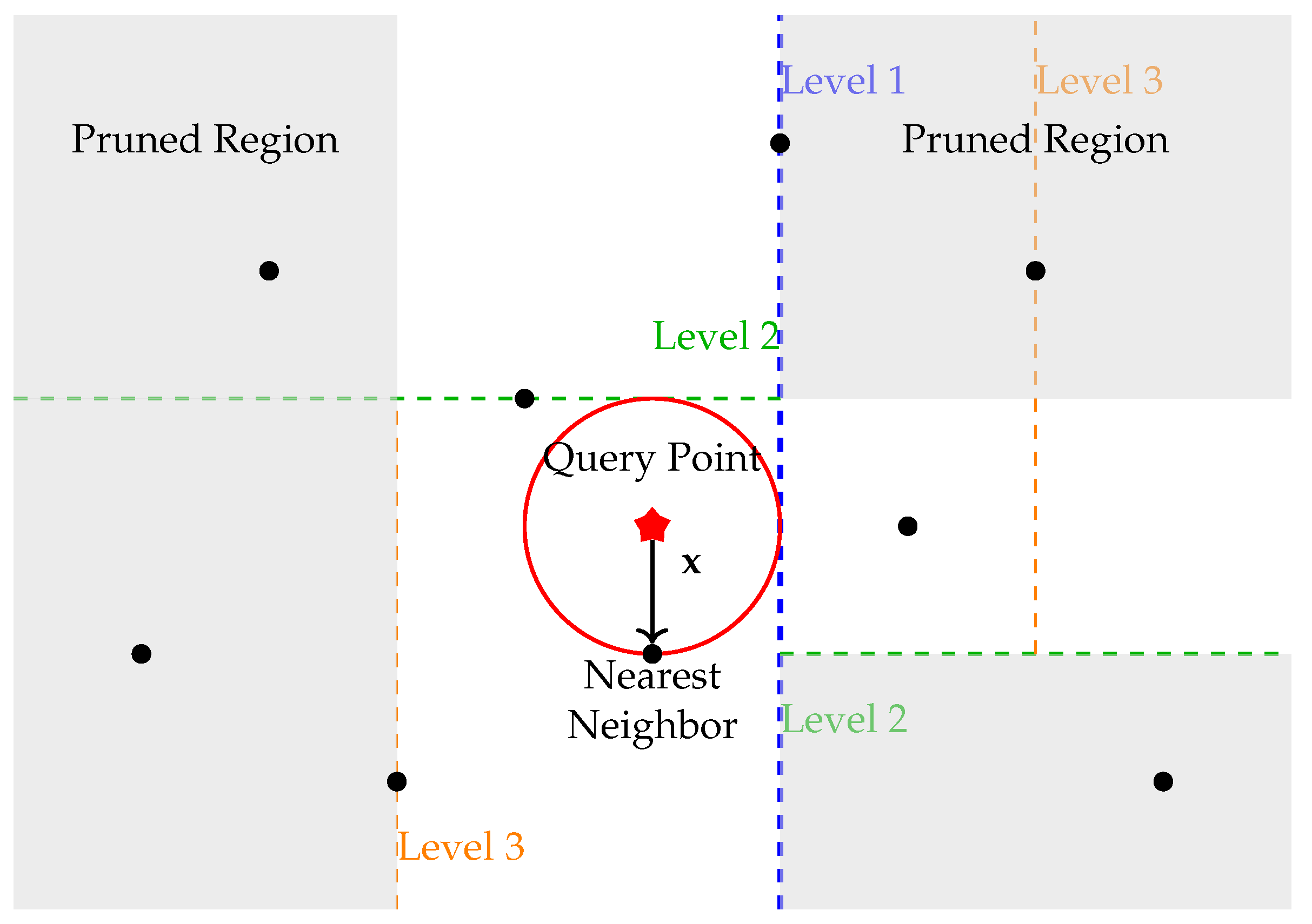
For example, when searching for the nearest neighbor to a query point , the KD-tree first identifies the region where resides. It then compares points within that region before expanding the search to neighboring regions only if necessary. This process avoids the need to compute distances to points in far-away regions, as the Euclidean distance between and points in those distant regions would exceed the distances already found in the current local region. This selective search process dramatically reduces the computational burden, especially in low- and moderate-dimensional spaces.
Figure 2 illustrates how a KD-tree partitions the space and reduces distance computations during nearest neighbor search. The query point
is located in a specific region, and the algorithm only needs to consider data points within that region and nearby regions that intersect the search radius. Pruned regions are shaded, showing how the KD-tree efficiently eliminates the need to compute distances to distant points. Building spatial data structures like KD-trees or Ball Trees can require significant memory, especially with large datasets or higher dimensions.
An alternative approach is the use of Approximate Nearest Neighbors (ANN) algorithms, which trade-off exactness for speed. Techniques such as Locality-Sensitive Hashing (LSH) [
39] enable faster searches by hashing data points into buckets based on random projections, ensuring that nearby points in the original space are more likely to be hashed into the same bucket. Although ANN algorithms do not guarantee the identification of the exact nearest neighbor, they offer significant computational savings and often suffice in practical applications.
Early Exit Strategies
Further optimizations can be achieved by leveraging techniques like early exit strategies in algorithms that do not require exact distances for all points. For instance, the additivity property of Euclidean distance in subspaces allows it to be broken down into the sum of squared differences across individual dimensions. This allows for partial distance calculations to determine if a point can be excluded early [
40]. If the partial sum of squared differences already exceeds a known threshold, further dimensions do not need to be considered. This is an effective optimization in high-dimensional spaces, where early termination of distance computation can save substantial computational effort.
Dimensionality Reduction Techniques
As datasets grow in size and dimensionality, traditional methods like Euclidean distance face increasing computational challenges. The
curse of dimensionality describes how the volume of space increases exponentially with the number of dimensions, causing data points to become sparse and distances less meaningful [
24]. This sparsity complicates tasks such as nearest neighbor searches, clustering, and classification, as computational costs escalate. In high-dimensional spaces, Euclidean distance often fails to effectively differentiate between nearby and distant points, prompting the need for alternative distance measures and mitigation techniques [
41].
To overcome these challenges, dimensionality reduction techniques are among the best options. These techniques aim to find a mapping , where , that preserves the essential geometric properties of the data while reducing the computational cost of distance calculations.
Principal Component Analysis (PCA) [
42] is one of the most widely used linear dimensionality reduction techniques. PCA transforms the original data points into a set of orthogonal components, ranked by the amount of variance they capture from the data. By retaining only the top
d components, where
, PCA effectively reduces the dimensionality of the data while preserving the most significant features, allowing for faster Euclidean distance computations [
43].
Another popular method is the t-Distributed Stochastic Neighbor Embedding (t-SNE) [
44], which is a non-linear technique designed to maintain the local structure of the data in a lower-dimensional space. While t-SNE is primarily used for visualization, it can also facilitate faster distance computations in the lower-dimensional embedding space, although with the trade-off of potentially altering global distances.
Random Projection [
45], grounded in the Johnson-Lindenstrauss Lemma, offers a probabilistic approach to dimensionality reduction. It projects the original data
onto a randomly chosen lower-dimensional subspace
using a random matrix
, where each entry
is independently drawn from a suitable distribution (e.g., Gaussian or sparse distribution):
This projection approximately preserves pairwise Euclidean distances with high probability:
where
is a small distortion parameter. Random Projection is particularly appealing due to its computational efficiency and simplicity, as it requires no prior knowledge of the data distribution and can be implemented with minimal overhead.
Dimensionality reduction techniques offer computational advantages but come with limitations. PCA, though effective for preserving variance, is a linear method and may miss complex, non-linear patterns. Its sensitivity to outliers can distort the data structure, and it may discard low-variance dimensions that are still important. t-SNE, useful for visualizing local structure, is computationally expensive and can distort global relationships, making it unsuitable for large datasets. Random Projection is efficient and easy to implement but introduces distortion in distances, potentially affecting accuracy, and its results can vary due to randomness. These techniques often involve trade-offs between efficiency, accuracy, and data-specific considerations.
Approximation via Clustering and Dimensional Culling
Instead of computing the exact distance matrix, one can use clustering techniques to approximate the distance matrix by grouping similar points together. For example, using cluster centroids as representatives for the points within each cluster, the distance matrix can be computed more efficiently by calculating distances between centroids rather than between individual points, which significantly reduces the number of required distance calculations [
46].
In high-dimensional spaces, not all dimensions contribute equally to the distance between points. Identifying and ignoring dimensions with low variance or limited impact on distance can reduce the number of calculations [
24].
3.2. Low-Level Optimizations
Low-level optimizations focus on improving the efficiency of Euclidean distance computations by optimizing the underlying code at a granular level. These optimizations are crucial when working with large-scale data or real-time systems where every computational cycle counts.
Approximation with Lower Precision
By applying scalar quantization to the individual dimensions of a vector, each component of the vector is approximated using lower precision. For scalar quantization, each component of the vector is mapped to a discrete set of values. This reduces the complexity of the distance calculation by performing operations on smaller, quantized values rather than the original high-precision numbers. For instance, instead of using floating-point arithmetic, the vector components are represented as integers, allowing faster calculations using integer arithmetic, which is typically more efficient in many hardware architectures [
47].
Scalar quantization maps each component of an n-dimensional vector to a quantized value , where is a finite set of levels. The resulting quantized value is defined as . In uniform quantization, the levels in are equally spaced. For L levels over the range , the quantization levels are given by , where and . The quantized value for is . The quantization error is the difference between and its quantized value: . Although this error accumulates in distance calculations, it allows for faster computations using lower precision.
Quantization lowers the precision of vector components, introducing some error in distance calculations. The coarser the quantization, the larger the potential error. This trade-off is acceptable in cases where exact precision is less important, such as approximate nearest neighbor searches or noisy data. It is especially beneficial in large-scale or real-time applications, where faster computation and reduced memory use outweigh the accuracy loss.
Loop Unrolling
Loop unrolling is another low-level optimization technique that can be applied to Euclidean distance calculations. By manually unrolling loops, the number of loop control instructions (such as incrementing indices and checking loop termination conditions) is reduced, allowing the CPU to perform more useful work per cycle [
48].
For example, consider the following loop that computes the squared Euclidean distance:
This loop can be unrolled by manually expanding the loop body for a fixed number of iterations:
While this increases the code size, it reduces the overhead of loop control and increases instruction-level parallelism, leading to faster execution.
Machine Code Optimization
Another avenue for optimizing Euclidean distance computations involves low-level programming and the use of just-in-time (JIT) compilers. Implementing distance calculations in low-level languages like C or C++ allows developers to exploit the full potential of the underlying hardware, using techniques such as assembly-level optimizations, manual loop unrolling, function inlining, instruction reordering, and precise control over memory allocation and access patterns to generate more efficient code [
49]. These optimizations can minimize cache misses and take advantage of specific CPU instructions that are optimized for floating-point arithmetic. By enabling these optimizations, further performance gains can be achieved without requiring manual intervention. In environments where floating-point computation is expensive, using fixed-point arithmetic can additionally reduce the computational load.
In addition to traditional low-level languages, Python developers can achieve similar performance gains by using Numba, a high-performance JIT compiler [
50]. Numba automatically translates Python functions into optimized machine code at runtime using the LLVM compiler library. This approach allows Python programs to reach speeds comparable to those of C or FORTRAN without requiring developers to leave the Python ecosystem. By simply applying a Numba decorator to a Python function, the function is automatically compiled into highly optimized machine code, often resulting in substantial speedups for numerical algorithms. This enables the efficient execution of distance calculations while retaining the flexibility and ease of use that Python offers.
Vectorization
Modern computing architectures offer vectorized instructions that can significantly accelerate distance calculations. Vectorization enables performing the same operation on multiple data elements simultaneously, leveraging the computational power of modern CPUs. Vectorized implementations and the use of advanced linear algebra libraries take advantage of special floating-point hardware, such as SIMD (Single Instruction, Multiple Data) operations and vector registers. By vectorizing the Euclidean distance computation, it is possible to leverage SIMD instructions to compute multiple distances in parallel within a single CPU core, thus speeding up the process [
51].
Libraries such as BLAS (Basic Linear Algebra Subprograms) and NumPy provide highly optimized routines for these vectorized operations, making them readily accessible for optimization. For instance, BLAS library implementations include a set of low-level routines for performing common linear algebra operations—like matrix multiplication, dot products, vector addition, scalar multiplication, norm computation, and sum reduction—which can be directly used to calculate Euclidean pairwise distance matrices.
NumPy is particularly advantageous for vectorizing Euclidean distance computations due to its ability to efficiently handle large arrays and matrices through optimized low-level implementations [
52]. These vectorized operations are built on highly optimized C libraries, allowing NumPy to fully leverage modern CPU architectures. By utilizing vectorization, NumPy can perform element-wise arithmetic across entire arrays simultaneously, significantly reducing the time complexity compared to traditional for-loop-based approaches in Python. This efficiency is further enhanced by the SIMD capabilities of modern CPUs, which enable the same operation to be applied to multiple data points in parallel. Additionally, NumPy’s integration with highly optimized linear algebra libraries, such as BLAS and LAPACK, ensures that operations like matrix multiplication and dot products—crucial for distance calculations—are executed with minimal overhead.
For example, vectorization techniques can be applied to distance calculations by expressing them in terms of matrix operations. The matrix of squared Euclidean distances between two vectors,
and
, is given by:
Here, represents the squared norm of , is the squared norm of , and denotes the dot product between and . Instead of performing full matrix multiplication, the squared norms and are computed more efficiently using row-wise operations. This optimization avoids unnecessary calculations, as only the squared norms for each row are required, significantly reducing the computational complexity.
Listing 1 provides an example of Python function for computing pairwise squared Euclidean distances between two sets of points using vectorization capabilities of NumPy library.
|
Listing 1: Python code for computing pairwise squared Euclidean distances between two sets of points using vectorization capabilities of NumPy
|
 |
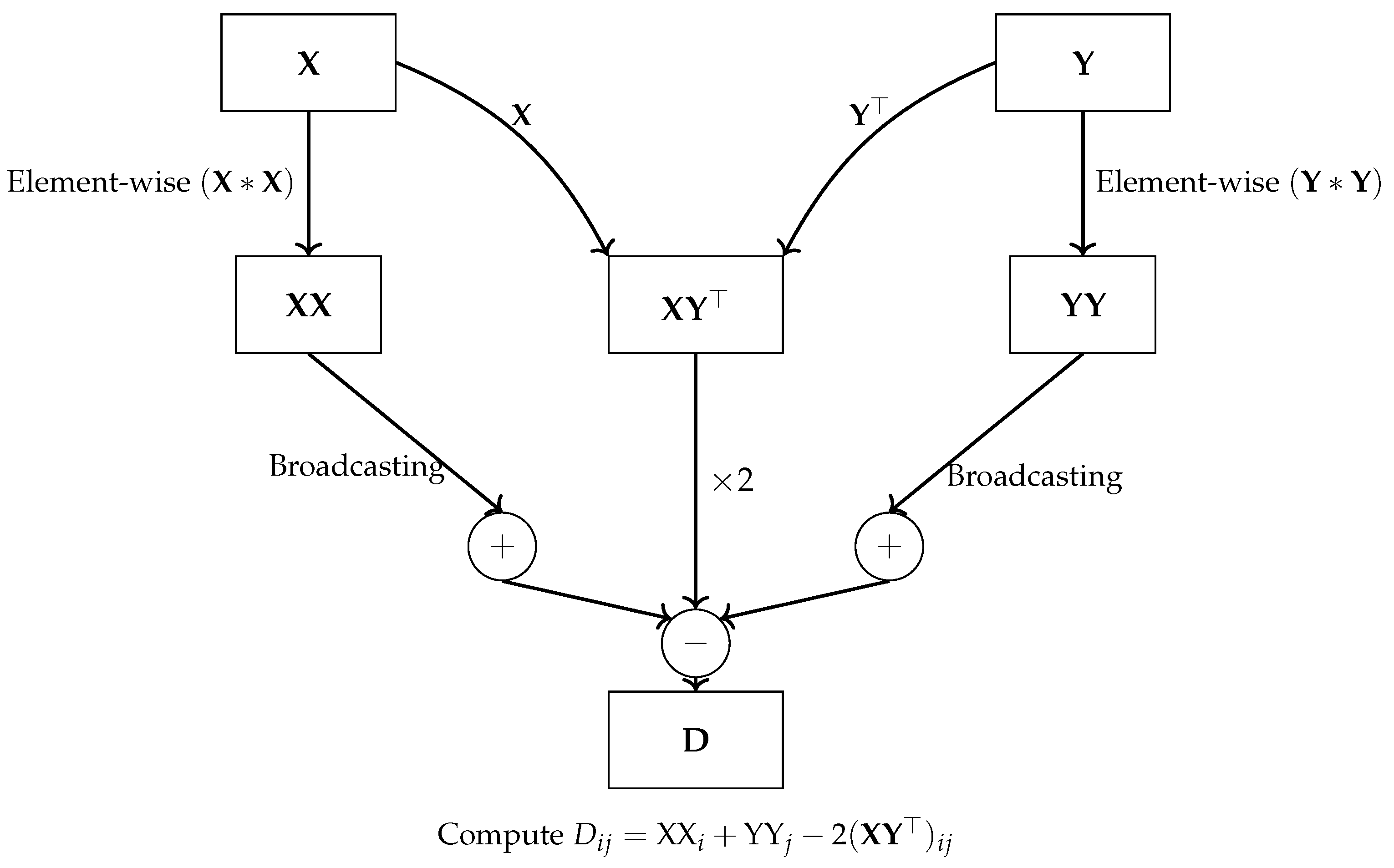
The vectorization capabilities of NumPy, as demonstrated in the code at Listing 1 and at
Figure 3, significantly accelerate the computation of pairwise squared Euclidean distances by avoiding explicit Python loops and leveraging highly optimized matrix operations.
In particular, the dot product between matrices and is computed using the function np.dot(X, Y.T), which takes advantage of NumPy’s efficient linear algebra routines to perform the operation in a single step across all pairs of points. Similarly, the squared norms of the rows in and are computed using SIMD element-wise multiplication operation () and sum reduction along the row dimension (axis=1), fully utilizing vectorized operations to handle entire arrays at once. The operation reshapes the 1D array into a 2D column vector, allowing NumPy to automatically expand the dimensions of and through broadcasting. In NumPy broadcasting enabling efficient element-wise operations with the 2D dot product result without explicitly copying data.
This approach eliminates the need for slow, iterative computations typically found in for-loop-based implementations. Instead, all operations are executed in parallel for each row of the matrices using special vector registers within a single CPU core, significantly boosting performance through SIMD operations. The final distance matrix is assembled by combining squared norms and dot products in a single vectorized expression, further optimizing computational efficiency.
Parallelization
Parallelization involves distributing the workload across multiple cores or processors, enabling simultaneous execution of distance calculations [
3]. This approach is particularly advantageous when dealing with large datasets or when Euclidean distance computation needs to be performed repeatedly, as in iterative algorithms like K-means clustering [
22] or K-nearest neighbors (KNN) [
53]. By breaking down the computation into smaller tasks that can be processed concurrently, parallelization reduces the overall computation time, making it feasible to handle more extensive datasets within a reasonable timeframe.
Parallelization is a powerful strategy for optimizing Euclidean distance calculations, particularly when dealing with large-scale data or computationally intensive algorithms. By effectively utilizing the available hardware resources—whether through multi-threading, multiprocessing, or distributed computing—parallelization can dramatically improve the performance and scalability of algorithms that rely on Euclidean distance measurements.
The main conceptual difference between CPU and GPU parallelism lies in their design: CPUs are optimized for sequential processing with a few powerful cores, focusing on complex tasks that require strong single-thread performance, whereas GPUs are designed for massive parallelism with thousands of smaller, simpler cores that excel at handling many simultaneous tasks, making them ideal for workloads like distance computations across large datasets [
53].
Libraries and frameworks like OpenMP for CPUs, CUDA for GPUs, and Apache Spark for distributed computing facilitate parallel computation by providing interfaces to efficiently utilize multiple cores, threads, and clusters, enhancing the performance of Euclidean distance calculations on various hardware architectures [
54].
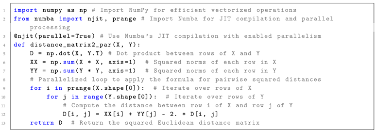
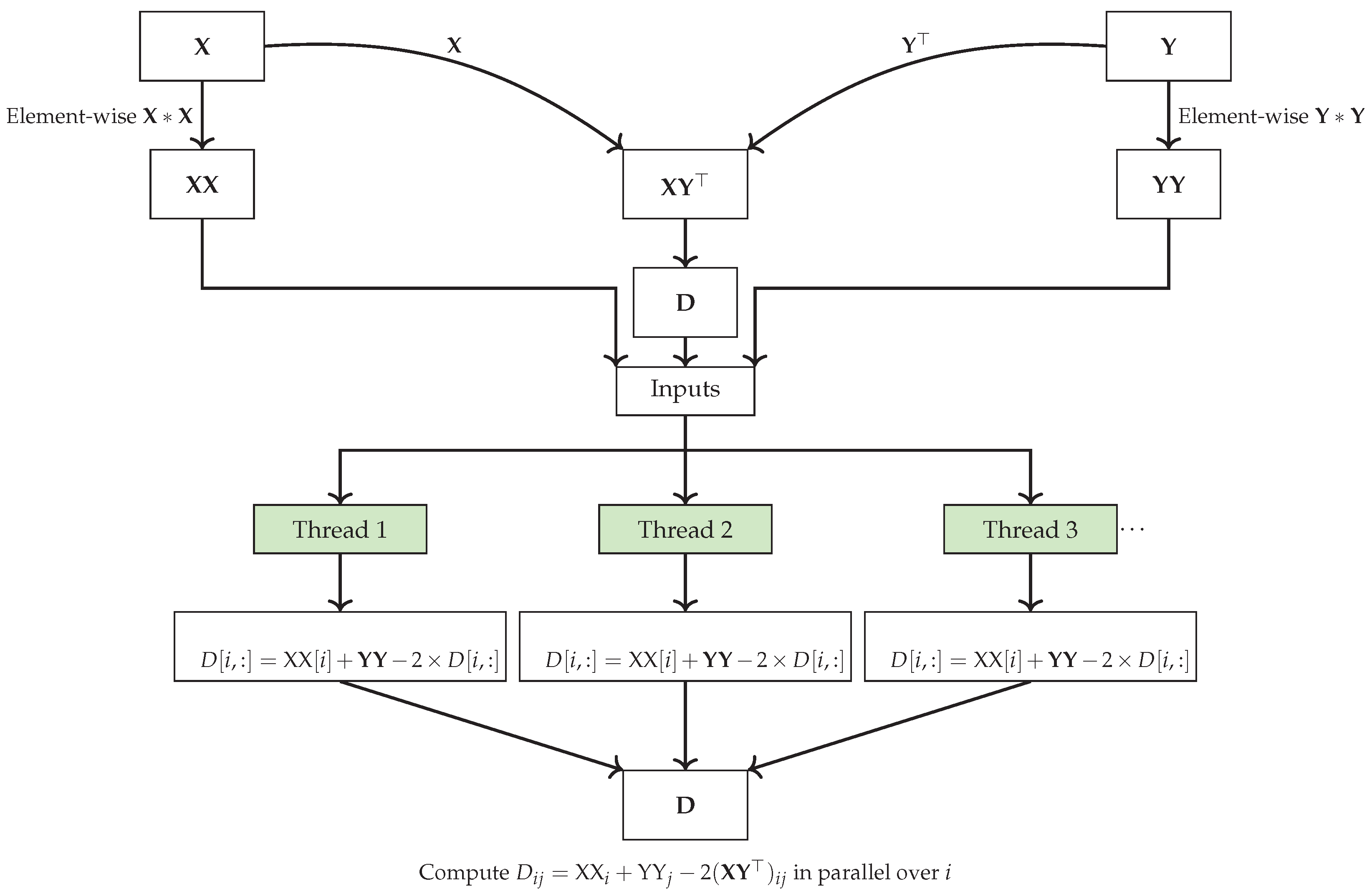
When combined with vectorization and machine code optimization, parallelization offers even greater potential for accelerating computations by leveraging modern hardware capabilities such as SIMD instructions, multi-core processors, and GPUs. By applying vectorized operations within each parallel thread or process, computational efficiency can be further enhanced, leading to significant reductions in processing time. Listing 2 provides an example of Python code for computing pairwise squared Euclidean distances between two sets of points using Numba’s JIT compilation. This approach combines automatic machine code optimization, vectorization, and parallelism across multiple CPU cores to enhance performance.
| Listing 2: Python code for computing pairwise squared Euclidean distances between two sets of points using Numba’s JIT compilation, which combines automatic machine code optimization, vectorization, and parallelism across multiple CPU cores for enhanced performance.
|
 |
In Listing 2, Numba’s JIT (Just-In-Time) compilation is applied to further accelerate the squared Euclidean distance computation compared to Listing 1. The @njit(parallel=True) decorator compiles the Python code into optimized machine code at runtime, allowing for faster execution by utilizing the CPU’s hardware capabilities. Parallelism is achieved through the prange construct, which distributes the workload of iterating over the rows of matrices X and Y across multiple CPU cores. This ensures that each core computes a portion of the pairwise distances, significantly speeding up the overall computation compared to the single-core, vectorized approach in Listing 1.
This parallelism significantly accelerates computation for larger datasets, especially when multiple CPU cores are utilized, as the pairwise distance calculations can be processed concurrently. As a result, the parallelization approach is particularly advantageous for large-scale problems, offering greater performance gains than vectorization alone, particularly when dealing with high-dimensional or large datasets and using multiple CPU or GPU cores. As the problem scale and the number of cores increase, the speedup achieved by parallelization can far exceed that of non-parallel implementations. However, when applied to small datasets, parallelization can increase memory usage due to the overhead of managing multiple threads or processes, as well as potential data duplication. Furthermore, combining vectorization and parallelization can yield extra efficiency by optimizing both individual arithmetic operations and the distribution of workload across cores, resulting in even greater overall acceleration.
Hardware Acceleration
Leveraging specialized hardware, such as multiple core CPUs and Graphics Processing Units (GPUs), can further accelerate Euclidean distance calculations [
53]. Modern GPUs consist of thousands of cores that can execute the same operation on multiple data points simultaneously, making them well-suited for tasks like Euclidean distance calculation where the same operation (distance computation) needs to be applied across many data points. GPUs, with their massively parallel architecture, are particularly beneficial for applications involving large datasets, where the parallel computing power of GPUs can dramatically reduce computation time.
Field-Programmable Gate Arrays (FPGAs) offer a different kind of hardware acceleration by allowing the user to create custom circuits that are optimized for specific tasks, such as Euclidean distance computation [
55]. Unlike GPUs, which are fixed-function devices, FPGAs can be reprogrammed to implement custom logic that executes the distance computations in an optimized fashion. FPGAs are particularly advantageous in applications where power efficiency is critical, as they can provide significant speedup with lower power consumption compared to GPUs or CPUs.
Figure 4.
Vectorized and parallelized computation of pairwise squared Euclidean distances using Numba’s JIT compilation and parallel processing.
Figure 4.
Vectorized and parallelized computation of pairwise squared Euclidean distances using Numba’s JIT compilation and parallel processing.
3.3. Hybrid Approaches
In practice, combining multiple optimization strategies often yields the best results. For instance, using dimensionality reduction to lower the computational burden, followed by squared distance optimization techniques to eliminate the square root operations, and then applying vectorization and parallelization can lead to significant speedups [
39]. Similarly, integrating hardware acceleration with algorithmic optimizations—such as spatial data structures and approximate methods—can maximize performance gains.
These hybrid approaches are particularly effective in large-scale applications, where combining different techniques allows for more scalable and efficient processing of complex datasets. By carefully selecting and integrating these optimization strategies, it is possible to tailor the computation of Euclidean distances to the specific needs of an application, achieving both high performance and accuracy [
56].
4. Comparative Analysis of Optimization Approaches
In this section, we compare the different optimization approaches discussed above in terms of their effectiveness, complexity, and suitability for various applications. The results of comparative analysis of optimization approaches for Euclidean distance computation are given in in
Table 1.
4.1. Computation Speedup
The primary goal of optimization is to reduce the time required to compute Euclidean distances. Techniques like squared Euclidean distance, advanced initialization, and lower-bound methods provide moderate to high speedups by eliminating redundant calculations or improving the initialization phase. Methods like early exit strategies, dimensional culling, and hardware acceleration can achieve very high speedups, particularly in large-scale or real-time applications.
4.2. Complexity
Most low-level techniques, such as loop unrolling, vectorization, and advanced initialization, have low to moderate complexity (ease of implementation) and are relatively straightforward to implement. More advanced strategies, such as recursive distance updating and approximate nearest neighbors, require deeper algorithmic understanding and expertise. Techniques like machine code optimization (e.g., using Numba) are moderately complex but can be automated through libraries, while hardware acceleration and FPGA usage demand specialized knowledge.
4.3. Scalability
Scalability is crucial in large-scale applications. Many of the techniques, like approximate nearest neighbors, vectorization, parallelization, and dimensional culling, scale well with large datasets. Precomputing distance matrices, while providing fast retrieval, may face scalability issues due to high memory usage in very large datasets. Parallelization techniques and spatial data structures (e.g., KD-trees) also scale well but may degrade in performance in high-dimensional data spaces.
4.4. Memory Usage
Techniques such as precomputing distance matrices and clustering involve high memory usage due to storing pairwise distances or intermediate results. In contrast, methods like vectorization, early exit strategies, and loop unrolling have minimal memory requirements, making them suitable for resource-constrained environments.
4.5. Hardware Requirements
Most approaches, such as advanced initialization, lower-bound techniques, and dimensionality reduction, can be implemented without specialized hardware. However, hardware acceleration approaches like GPU and FPGA acceleration require appropriate hardware resources. Similarly, vectorization benefits from SIMD-enabled CPUs, and parallelization thrives with multi-core processors or GPU support.
4.6. Accuracy Impact
Accuracy impact refers to the trade-offs between computational speed and precision. Techniques like squared Euclidean distance, lower-bound methods, triangle inequality, and vectorization maintain exact accuracy while improving efficiency. In contrast, methods such as approximate nearest neighbors (ANN), dimensionality reduction, and lower precision approximations may introduce slight inaccuracies, suitable for cases where faster computation outweighs precision. Techniques like parallelization and hardware acceleration preserve accuracy when properly implemented. The choice depends on the application’s tolerance for accuracy loss versus the need for speed.
4.7. Best Use Cases
The suitability of each approach depends on the specific application. Each technique has ideal use cases. Advanced initialization works best for algorithms like K-means where a good initial guess speeds up convergence. Early exit strategies are highly effective for high-dimensional nearest neighbor searches, while dimensional culling excels in high-dimensional spaces where not all dimensions contribute equally. Loop unrolling and vectorization are best for low-level numerical optimizations, and hardware acceleration is critical for real-time or large-scale processing tasks.
5. Discussion
Selecting the appropriate optimization technique for Euclidean distance computations depends on the specific data characteristics and application requirements. Techniques like squared Euclidean distance, lower-bound methods, and triangle inequality are effective for algorithms such as K-means clustering and K-nearest neighbors, where exact distance calculations are crucial. These methods provide significant speedups without sacrificing accuracy, making them ideal for large datasets that demand precision.
Spatial data structures like KD-trees and Ball Trees efficiently partition space to accelerate nearest neighbor searches in low to moderate-dimensional data. However, their performance diminishes in high-dimensional spaces due to the curse of dimensionality. For high-dimensional data, dimensionality reduction techniques and clustering with dimensional culling become more appropriate. Methods like Principal Component Analysis or Random Projection reduce data to a lower-dimensional space, preserving significant variance while decreasing computation time, suitable for exploratory data analysis or preprocessing in machine learning pipelines.
Approximate methods, including Locality-Sensitive Hashing, are advantageous when exact nearest neighbor searches are computationally infeasible due to dataset size. They offer substantial speedups with acceptable accuracy loss, making them suitable for applications like recommendation systems or real-time search where response time is critical. Hardware acceleration techniques, such as GPU and FPGA implementations, leverage parallel processing capabilities to significantly reduce computation times while maintaining accuracy, making them effective for real-time processing and handling large-scale data in environments like deep learning and big data analytics.
A critical consideration in selecting an optimization approach is balancing computation speed and potential loss of accuracy. Techniques that introduce approximations—such as approximate nearest neighbors, dimensionality reduction, and approximation with lower precision—may impact accuracy. While these methods offer high speedups, they may not be suitable for applications where precise distance calculations are essential, such as in medical imaging or security-sensitive domains. Conversely, methods like vectorization, parallelization, and machine code optimization provide significant computational benefits without compromising accuracy, making them ideal for applications requiring both high performance and precise results.
When employing clustering and dimensional culling, there’s a trade-off between reducing computational load and the risk of losing important information in the omitted dimensions. This can impact accuracy, particularly if the discarded dimensions are relevant to the analysis. Assessing the significance of each dimension is crucial in the context of the specific application.
The choice of optimization technique also depends on available computational resources. Hardware acceleration methods require specialized hardware like GPUs or FPGAs, which may not be feasible in all settings due to cost or infrastructure limitations. In such cases, software-based optimizations like vectorization or loop unrolling can still provide substantial speedups on standard CPUs. Parallelization offers high scalability and is effective for large datasets but may increase memory usage due to overhead from managing multiple threads or processes. Applications with limited memory resources need to consider this trade-off. For static datasets where repeated distance computations are required, precomputing and caching distances can significantly speed up retrieval times, but this approach demands high memory usage, which might not be suitable for extremely large datasets or memory-constrained environments.
Ultimately, selecting the most appropriate optimization strategy requires understanding the application’s specific needs and constraints. For applications where accuracy is paramount and computational resources are ample, methods that preserve exact distances while optimizing computation—such as vectorization and parallelization—are preferable. In scenarios where computational speed is critical and some accuracy loss is acceptable, approximate methods and dimensionality reduction techniques may be more suitable. Evaluating the impact of potential inaccuracies on the application’s outcomes is essential. Combining multiple optimization approaches can yield tailored solutions that align closely with specific requirements and limitations.
6. Conclusion
As data sizes and algorithmic complexity continue to grow, advancements in optimization techniques will be crucial for improving the performance of algorithms that rely on Euclidean distance calculations. Although Euclidean distance computation is simple in its formulation, it can become a significant computational bottleneck in large-scale applications. Optimizing this operation can greatly improve the overall efficiency of various analytical processes. By reducing the time and computational resources required for distance calculations, these optimizations will improve the scalability and responsiveness of data-driven applications. Additionally, increased computational efficiency directly translates to lower energy consumption, making these optimizations essential for minimizing the environmental impact of large-scale data processing. As energy efficiency is a key component of sustainable development, the reduction in power usage achieved through optimizing Euclidean distance calculations supports global efforts toward more eco-friendly and sustainable technological solutions.
This paper has reviewed and compared various optimization techniques aimed at accelerating Euclidean distance computations. These techniques span algorithm-specific optimizations, low-level code optimizations, and hardware acceleration, each offering different trade-offs in terms of speed, complexity, and resource requirements.
Applying these optimization techniques provides distinct advantages depending on the specific use case. Algorithm-specific methods, like squared Euclidean distance and lower-bound techniques, allow for immediate reductions in computation time without significant changes in implementation complexity, making them well-suited for standard machine learning tasks. Low-level optimizations such as vectorization, loop unrolling, and parallelization exploit modern CPU architectures for rapid computations, particularly useful in high-throughput environments. Meanwhile, hardware acceleration using GPUs or FPGAs offers the most significant speedups for real-time applications or large datasets, although they come with higher development and hardware costs. Together, these techniques allow practitioners to tailor solutions that maximize performance based on available resources, dataset size, and application demands. By comparing the effectiveness, complexity, and scalability of various optimization techniques, our findings guide practitioners in selecting the most suitable methods for improving Euclidean distance computations in their specific contexts.
This comparative analysis highlights that no single optimization technique is universally superior. The best optimization strategy depends on dataset size, dimensionality, memory constraints, and the availability of hardware resources. Combining multiple techniques often offers the most efficient and scalable solution for improving Euclidean distance computations, particularly in large-scale machine learning and data analysis applications.
As data sizes continue to grow and applications become more demanding, the importance of efficient Euclidean distance computation will only increase. Future research may focus on developing hybrid methods that combine multiple optimization strategies or on leveraging emerging hardware technologies, such as quantum computing, to further accelerate these computations. The continued development of efficient Euclidean distance computation techniques will remain a critical area of research, enabling advancements across numerous scientific and engineering disciplines.
Funding
This research was funded by the Science Committee of the Ministry of Science and Higher Education of the Republic of Kazakhstan (grant no. BR21882268).
Data Availability Statement
Conflicts of Interest
The authors declare no conflicts of interest.
Abbreviations
The following abbreviations are used in this manuscript:
| ANN |
Approximate Nearest Neighbors |
| BLAS |
Basic Linear Algebra Subprograms |
| CPU |
Central Processing Unit |
| CUDA |
Compute Unified Device Architecture |
| FPGA |
Field-Programmable Gate Array |
| GPU |
Graphics Processing Unit |
| JIT |
Just-In-Time |
| KNN |
K-Nearest Neighbors |
| KD-tree |
K-Dimensional Tree |
| LSH |
Locality-Sensitive Hashing |
| MSSC |
Minimum Sum-of-Squares Clustering |
| OpenMP |
Open Multi-Processing |
| PCA |
Principal Component Analysis |
| SIMD |
Single Instruction, Multiple Data |
| t-SNE |
t-Distributed Stochastic Neighbor Embedding |
References
- Deza, M.M.; Deza, E. Encyclopedia of Distances, 4 ed.; Springer: Berlin, Heidelberg, 2016; p. 756. [Google Scholar] [CrossRef]
- Bottesch, T.; Bühler, T.; Kächele, M. Speeding up k-means by approximating Euclidean distances via block vectors. International conference on machine learning; PMLR, 2016; pp. 2578–2586. [Google Scholar]
- Mussabayev, R.; Mussabayev, R. Superior Parallel Big Data Clustering Through Competitive Stochastic Sample Size Optimization in Big-Means. Intelligent Information and Database Systems; Nguyen, N.T., Chbeir, R., Manolopoulos, Y., Fujita, H., Hong, T.P., Nguyen, L.M., Wojtkiewicz, K., Eds.; Springer Nature Singapore: Singapore, 2024; pp. 224–236. [Google Scholar] [CrossRef]
- Liberti, L.; Lavor, C. Euclidean distance geometry; Springer, 2017; Volume 3. [Google Scholar]
- Croom, F.H. Principles of topology; Courier Dover Publications, 2016. [Google Scholar]
- Braga-Neto, U. Fundamentals of pattern recognition and machine learning; Springer, 2020. [Google Scholar]
- Oyewole, G.J.; Thopil, G.A. Data clustering: application and trends. Artificial Intelligence Review 2023, 56, 6439–6475. [Google Scholar] [CrossRef] [PubMed]
- Varoquaux, G.; Buitinck, L.; Louppe, G.; Grisel, O.; Pedregosa, F.; Mueller, A. Scikit-learn: Machine learning without learning the machinery. GetMobile: Mobile Computing and Communications 2015, 19, 29–33. [Google Scholar] [CrossRef]
- Burger, W.; Burge, M.J. Digital image processing: An algorithmic introduction; Springer Nature, 2022. [Google Scholar]
- Tolebi, G.; Dairbekov, N.S.; Kurmankhojayev, D.; Mussabayev, R. Reinforcement learning intersection controller. 2018 14th International Conference on Electronics Computer and Computation (ICECCO); IEEE, 2018; pp. 206–212. [Google Scholar]
- Fischer, M.M.; Scholten, H.J.; Unwin, D. Geographic information systems, spatial data analysis and spatial modelling: an introduction. In Spatial analytical perspectives on GIS; Routledge, 2019; pp. 3–20. [Google Scholar]
- Tang, Y.; Zhao, L.; Zhang, S.; Gong, C.; Li, G.; Yang, J. Integrating prediction and reconstruction for anomaly detection. Pattern Recognition Letters 2020, 129, 123–130. [Google Scholar] [CrossRef]
- Eiselt, H.A.; Sandblom, C.L. Decision analysis, location models, and scheduling problems; Springer Science & Business Media, 2013. [Google Scholar]
- Carter, C.R.; Rogers, D.S.; Choi, T.Y. Toward the theory of the supply chain. Journal of supply chain management 2015, 51, 89–97. [Google Scholar] [CrossRef]
- Perfilyeva, A.; Bespalova, K.; Kuzovleva, Y.; Mussabayev, R.; et al. . Genetic diversity and origin of Kazakh Tobet Dogs. Scientific Reports 2024, 14, 23137. [Google Scholar] [CrossRef]
- van den Belt, M.; Gilchrist, C.; Booth, T.J.; Chooi, Y.H.; Medema, M.H.; Alanjary, M. CAGECAT: The CompArative GEne Cluster Analysis Toolbox for rapid search and visualisation of homologous gene clusters. BMC bioinformatics 2023, 24, 181. [Google Scholar] [CrossRef]
- Mussabayev, R. Colour-based object detection, inverse kinematics algorithms and pinhole camera model for controlling robotic arm movement system. 2015 Twelve International Conference on Electronics Computer and Computation (ICECCO); IEEE, 2015; pp. 1–9. [Google Scholar]
- Mukhamediev, R.I.; Yakunin, K.; Aubakirov, M.; Assanov, I.; Kuchin, Y.; Symagulov, A.; Levashenko, V.; Zaitseva, E.; Sokolov, D.; Amirgaliyev, Y. Coverage path planning optimization of heterogeneous UAVs group for precision agriculture. IEEE Access 2023, 11, 5789–5803. [Google Scholar] [CrossRef]
- Bojanowski, P.; Grave, E.; Joulin, A.; Mikolov, T. Enriching word vectors with subword information. Transactions of the association for computational linguistics 2017, 5, 135–146. [Google Scholar] [CrossRef]
- Li, J.; Wu, L.; Hong, R.; Hou, J. Random walk based distributed representation learning and prediction on social networking services. Information Sciences 2021, 549, 328–346. [Google Scholar] [CrossRef]
- Altman, N.; Krzywinski, M. The curse (s) of dimensionality. Nat Methods 2018, 15, 399–400. [Google Scholar] [CrossRef]
- Mussabayev, R.; Mladenovic, N.; Jarboui, B.; Mussabayev, R. How to use K-means for big data clustering? Pattern Recognition 2023, 137, 109269. [Google Scholar] [CrossRef]
- Uddin, S.; Haque, I.; Lu, H.; Moni, M.A.; Gide, E. Comparative performance analysis of K-nearest neighbour (KNN) algorithm and its different variants for disease prediction. Scientific Reports 2022, 12, 6256. [Google Scholar] [CrossRef]
- Aggarwal, C.C.; Hinneburg, A.; Keim, D.A. On the surprising behavior of distance metrics in high dimensional space. Database theory—ICDT 2001: 8th international conference, 2001 proceedings 8. London, UK, 4-6 January 2001; Springer, 2001; pp. 420–434. [Google Scholar]
- Maitrey, S.; Jha, C. MapReduce: simplified data analysis of big data. Procedia Computer Science 2015, 57, 563–571. [Google Scholar] [CrossRef]
- Qi, Z.; Xiao, Y.; Shao, B.; Wang, H. Toward a distance oracle for billion-node graphs. Proceedings of the VLDB Endowment 2013, 7, 61–72. [Google Scholar] [CrossRef]
- Elkan, C. Using the triangle inequality to accelerate k-means. In Proceedings of the 20th international conference on Machine Learning (ICML-03); 2003; pp. 147–153. [Google Scholar]
- Contreras, P.; Murtagh, F. Hierarchical clustering; 2015; pp. 103–124. [Google Scholar] [CrossRef]
- Bentley, J.L. Multidimensional binary search trees used for associative searching. Commun. ACM 1975, 18, 509–517. [Google Scholar] [CrossRef]
- Omohundro, S.M. Five Balltree Construction Algorithms. Technical Report TR-89-063; International Computer Science Institute, 1989. [Google Scholar]
- Bock, H.H. Origins and extensions of the k-means algorithm in cluster analysis. Electronic journal for history of probability and statistics 2008, 4, 1–18. [Google Scholar]
- Ying, Y.; Li, P. Distance metric learning with eigenvalue optimization. The Journal of Machine Learning Research 2012, 13, 1–26. [Google Scholar]
- Cormen, T.H.; Leiserson, C.E.; Rivest, R.L.; Stein, C. Introduction to algorithms; MIT press, 2022. [Google Scholar]
- Fränti, P.; Sieranoja, S. How much can k-means be improved by using better initialization and repeats? Pattern Recognition 2019, 93, 95–112. [Google Scholar] [CrossRef]
- Hamerly, G. Making k-means even faster. In Proceedings of the 2010 SIAM International Conference on Data Mining (SDM); SIAM, 2010; pp. 130–140. [Google Scholar] [CrossRef]
- Jeon, Y.; Yoon, S. Multi-Threaded Hierarchical Clustering by Parallel Nearest-Neighbor Chaining. IEEE Transactions on Parallel and Distributed Systems 2015, 26, 2534–2548. [Google Scholar] [CrossRef]
- Arthur, D.; Vassilvitskii, S. k-means++: The advantages of careful seeding. In Proceedings of the eighteenth annual ACM-SIAM symposium on Discrete algorithms; SIAM, 2007; pp. 1027–1035. [Google Scholar]
- Park, H.S.; Jun, C.H. A simple and fast algorithm for K-medoids clustering. Expert systems with applications 2009, 36, 3336–3341. [Google Scholar] [CrossRef]
- Indyk, P.; Motwani, R. Approximate nearest neighbors: towards removing the curse of dimensionality. Proceedings of the Thirtieth Annual ACM Symposium on Theory of Computing; Association for Computing Machinery: New York, NY, USA, 1998; STOC’98; pp. 604–613. [Google Scholar] [CrossRef]
- McNames, J. Rotated partial distance search for faster vector quantization encoding. IEEE Signal Processing Letters 2000, 7, 244–246. [Google Scholar] [CrossRef]
- Beyer, K.; Goldstein, J.; Ramakrishnan, R.; Shaft, U. When is “nearest neighbor” meaningful? Database Theory—ICDT’99: 7th International Conference Jerusalem, Israel, 10-12 January 1999; Proceedings 7. Springer, 1999; pp. 217–235. [Google Scholar]
- Jolliffe, I.T.; Cadima, J. Principal component analysis: a review and recent developments. Philosophical Transactions of the Royal Society A: Mathematical, Physical and Engineering Sciences 2016, 374, 20150202. [Google Scholar] [CrossRef]
- Gewers, F.L.; Ferreira, G.R.; Arruda, H.F.D.; Silva, F.N.; Comin, C.H.; Amancio, D.R.; Costa, L.d.F. Principal component analysis: A natural approach to data exploration. ACM Computing Surveys (CSUR) 2021, 54, 1–34. [Google Scholar] [CrossRef]
- van der Maaten, L.; Hinton, G. Visualizing Data using t-SNE. Journal of Machine Learning Research 2008, 9, 2579–2605. [Google Scholar]
- Bingham, E.; Mannila, H. Random projection in dimensionality reduction: applications to image and text data. Knowledge Discovery and Data Mining 2001. [Google Scholar] [CrossRef]
- Borodin, A.; Ostrovsky, R.; Rabani, Y. Subquadratic approximation algorithms for clustering problems in high dimensional spaces. Machine Learning 2004, 56, 153–167. [Google Scholar] [CrossRef]
- Rodriguez, A.; Segal, E.; Meiri, E.; Fomenko, E.; Kim, Y.J.; Shen, H.; Ziv, B. Lower numerical precision deep learning inference and training. Intel White Paper 2018, 3, 1–19. [Google Scholar]
- Lee, S.; Gerstlauer, A. Data-dependent loop approximations for performance-quality driven high-level synthesis. IEEE Embedded Systems Letters 2017, 10, 18–21. [Google Scholar] [CrossRef]
- Pikus, F.G. The Art of Writing Efficient Programs: An advanced programmer’s guide to efficient hardware utilization and compiler optimizations using C++ examples; Packt Publishing Ltd, 2021. [Google Scholar]
- Lam, S.K.; Pitrou, A.; Seibert, S. Numba: A llvm-based python jit compiler. In Proceedings of the Second Workshop on the LLVM Compiler Infrastructure in HPC; 2015; pp. 1–6. [Google Scholar]
- Patterson, D.A.; Hennessy, J.L. Computer Architecture: A Quantitative Approach, 5th ed.; The Morgan Kaufmann Series in Computer Architecture and Design, Elsevier Science & Technology; 2011. [Google Scholar]
- Harris, C.R.; Millman, K.J.; Van Der Walt, S.J.; Gommers, R.; Virtanen, P.; Cournapeau, D.; Wieser, E.; Taylor, J.; Berg, S.; Smith, N.J.; others. Array programming with NumPy. Nature 2020, 585, 357–362. [Google Scholar] [CrossRef]
- Masek, J.; Burget, R.; Karasek, J.; Uher, V.; Dutta, M.K. Multi-GPU implementation of k-nearest neighbor algorithm. 2015 38th International Conference on Telecommunications and Signal Processing (TSP); IEEE, 2015; pp. 764–767. [Google Scholar]
- Dean, J.; Ghemawat, S. MapReduce: simplified data processing on large clusters. Commun. ACM 2008, 51, 107–113. [Google Scholar] [CrossRef]
- Boikos, K.; Bouganis, C.S. A scalable fpga-based architecture for depth estimation in slam. International Symposium on Applied Reconfigurable Computing; Springer, 2019; pp. 181–196. [Google Scholar]
- Gribel, D.; Vidal, T. HG-means: A scalable hybrid genetic algorithm for minimum sum-of-squares clustering. Pattern Recognition 2019, 88, 569–583. [Google Scholar] [CrossRef]
Short Biography of Authors
 |
Rustam Mussabayev is an Associate Professor and the Head of the AI Research Lab at Satbayev University, Kazakhstan. He holds a Candidateof Engineering Sciences degree(equivalent to a PhD in Computer Science) with expertise in datascience, high-performance computing, and operations research. His research interests span a wide range of topics, including clustering, natural language processing, machine learning, and optimization. He has received numerous awards, including the StatePrize “Best Researcher 2023” of the Republic of Kazakhstan and the Best Paper Award at ACIIDS 2024. His work is widely published in top-tier journals and conferences, contributing to advancements in data analysis, algorithm development, and high-performance computing solutions. |
|
Disclaimer/Publisher’s Note: The statements, opinions and data contained in all publications are solely those of the individual author(s) and contributor(s) and not of MDPI and/or the editor(s). MDPI and/or the editor(s) disclaim responsibility for any injury to people or property resulting from any ideas, methods, instructions or products referred to in the content. |
© 2024 by the authors. Licensee MDPI, Basel, Switzerland. This article is an open access article distributed under the terms and conditions of the Creative Commons Attribution (CC BY) license (http://creativecommons.org/licenses/by/4.0/).
