Aggressive Monetary and Fiscal Policy Impact on Household Wealth: A Comparative Analysis of China and Japan

Preprint

Article

Aggressive Monetary and Fiscal Policy Impact on Household Wealth: A Comparative Analysis of China and Japan

Altmetrics

Downloads

Views

Comments

RUIZHE HU^*

This version is not peer-reviewed

Submitted:

10 October 2024

Posted:

11 October 2024

You are already at the latest version

Alerts

Abstract

This paper uses a Vector Autoregression (VAR) model and linear regression to analyze the effects of aggressive monetary policies (such as RRR cuts and interest rate reductions) and fiscal measures (like government bond issuance) on household wealth in China, with a focus on housing assets. A comparative analysis with Japan is conducted to explore the transmission mechanisms and the policies’ impacts on housing prices, wealth distribution, and economic growth. The findings highlight the significant role of monetary and fiscal interventions in shaping the housing market dynamics across different economic contexts.

Keywords:

Subject: Business, Economics and Management - Economics

1. Introduction

Many economists recognize the crucial role of real estate markets in economic growth, as they influence capital and land—key production factors. In recent years, China has adopted aggressive monetary and fiscal measures to counter economic slowdown. For instance, on September 27, 2024, the People’s Bank of China (PBoC) cut the reserve requirement ratio by 0.5 percentage points, injecting around 1 trillion yuan in liquidity, and reduced the 7-day reverse repo rate by 0.2 percentage points to lower financing costs and stimulate the real economy. Additionally, long-term government bonds issued in May were allocated to national infrastructure projects to support growth.

Household wealth in China is primarily composed of financial assets and housing, with housing making up a significant portion. Research indicates that housing wealth significantly affects household consumption and wealth distribution. By influencing financial and real estate markets, monetary and fiscal policies directly impact household wealth dynamics.

This paper uses a Vector Autoregression (VAR) model and linear regression to analyze the effects of aggressive monetary policies (such as RRR cuts and interest rate reductions) and fiscal measures (like government bond issuance) on household wealth in China, focusing on housing assets. A comparative analysis with Japan is conducted to explore the transmission mechanisms and the policies’ impacts on housing prices, wealth distribution, and economic growth.

2. Literature Review

The housing market’s cyclical factor is one of major factor that decide the housing price. There were many research paper studied the cyclical effect. Pyhrr et al. (1999) explored various real estate cycle models and their strategic importance, emphasizing that understanding the dynamics of these cycles is essential for achieving above-average market returns [1]. Kaiser (1997) analyzed long-term cycles spanning 50 to 60 years, identifying inflation and overbuilding as key drivers, and suggested that understanding these long cycles could help optimize investment timing [2]. Other than the cyclical factor, the housing price also has significant relationship with macroeconomic factor. Ewing and Payne (2005) provided empirical evidence showing that macroeconomic shocks, such as changes in monetary policy, inflation, and output fluctuations, significantly impact the returns of real estate investment trusts (REITs) [3]. For regional study and asian countries, Nguyen et al. (2019) analyzed the relationship between the real estate market and economic growth in Vietnam [4]. Cellmer et al. (2019) investigated the dynamic interactions between housing prices and macroeconomic variables such as inflation, unemployment, and GDP in Poland. Using VAR and Granger causality tests, the study found that housing prices do strongly react to economic shocks [5].Not only moneatry policy will affect the real estate market, fiscal policy also has strong influence. According to Ju Fang et al. (2013), regional differences significantly influence how land transfer revenue and fiscal expenditure affect housing prices. In economically developed areas, higher land transfer revenue tends to drive up housing prices.[6]. However, still most of the article discuss from monetary policy side, and this article will introduce the newly issued government bond as one factor affect housing price.

3. Research Methodology

VAR (Vector Autoregression) models have become a fundamental tool in macroeconomic analysis due to their flexibility and ability to model the dynamic relationships among multiple time series without imposing strict causal assumptions. Introduced by Sims (1980), VAR models allow all variables in the system to be treated as endogenous, capturing the interdependencies and feedback mechanisms among them [7]. Nakajima (2011) emphasized that advanced versions of VAR, such as the Time-Varying Parameter VAR (TVP-VAR) with stochastic volatility, enhance the model’s ability to account for changes in economic structures over time, making it suitable for analyzing economies undergoing significant structural shifts [8]. The stochastic volatility component allows for the accommodation of fluctuations in shock variances, improving estimation accuracy through Bayesian methods like Markov Chain Monte Carlo (MCMC).

Jacobson et al. (1999) further demonstrated the practical application of VAR models in analyzing monetary policy within small open economies. By applying long-run restrictions and cointegration techniques, VAR models can distinguish between short-term and long-term impacts of monetary policy shocks on variables such as exchange rates, interest rates, and inflation. This approach provides insights into how economic policies propagate through different channels, making VAR models crucial for policy analysis and forecasting [9].

Building on these methodologies, this research utilizes macroeconomic time series data sourced from the CEIC website, covering variables such as housing prices, interest rates, SHIBOR, and new government bond issuances for China and Japan from 2000 to 2023. The time series data is tested for stationarity using the Augmented Dickey-Fuller (ADF) test, and the Johansen cointegration test is applied to identify any long-run equilibrium relationships. For cointegrated series, Vector Error Correction Models (VECM) are used to capture short-term dynamics. Additionally, a TVP-VAR model is employed to reflect the evolving economic structure and analyze the dynamic interactions more accurately. Impulse response functions are then utilized to assess the effects of shocks on macroeconomic variables, providing a comprehensive understanding of the interactions between macroeconomic indicators and housing markets.

Now We can define the total household wealth function which is:

W = F + H + C + R

(1)

Where:

W is the total household wealth,
F is the financial assets (including cash, stocks, bonds, etc.),
H is the real estate assets (including housing and commercial property),
C represents other constant assets,
R represents the residual, capturing other variables not explicitly studied.

We can also build a equation for house price base on the theory:

H_{t} = H_{t - 1} + C + α_{1} * I + β_{1} * Δ * B + ϵ_{1}

(2)

Where:

$H_{t}$ is the housing today price,
B is government bonds,
$Δ * B$ is the newly issued government bond,
I is the market interest,
C represents constant number,
$ϵ$ represents the residual.
$H_{t - 1}$ represents the housing price from the previous period.

We can also build a equation for financial asset price base on the theory:

4. Housing

Housing is the most important part of people’s wealth in East Asia. The fluctuation of Housing price will significantly affect Household’s pattern of consumption and investment. The boost in real estate market will improve leverage which have positive effect on Household consumption. The consumption will also improve the National Economy. Base on the economic datas and articles, the real estate market shows the cyclical phenomenon and a general trend which has a fix direction. We assume the price of the housing is composed by two part: Cyclical Factor and General Trend.

H = κ + C + T + ϵ_{H}

(3)

Where:

H is housing price,
C is Cyclical Factor,
T is General Trend,
$ϵ_{H}$ is residual,
$κ$ is constant,

4.1. Cyclical Phenomenon of Housing Price

The Cyclical Phenomenon of real estate market are well recognized. Most of the asian country (PRC, ROC, Singapore and Japan) all shows the cylical in their price. This article will re-studied the Housing price in China and Japan with newer data. Depend on the figures below, We can set a cyclical function for cyclical real estate market:

C_{t} = c + α * sin (w * T + ϕ) + ϵ_{c}

(4)

Where:

c is the constant,
$α$ is amplitude,
w is Angular frequency,
T is the period,
$ϕ$ is the Propagation constant,
$ϵ_{c}$ represents the residual.

Figure 1. Cyclical effect in Japan.

Figure 2. Cyclical Effect in China.

Figure 3. General Trend for JP housing price.

Figure 4. General Trend for CN housing price.

4.2. VAR model of Housing Price for Interest rate ( $Δ$ Trend)

The Vector Autoregression (VAR) model is a popular tool used to study the dynamic relationships between multiple macroeconomic variables, such as housing prices, leverage, and consumption. It allows for the analysis of how changes in one variable, like monetary policy adjustments or housing prices, influence other factors over time. In recent studies, this method has been applied to explore the interaction between housing prices and economic conditions in various markets. For instance, fluctuations in China’s housing prices have been closely linked to changes in consumer behavior and leverage [10]. Additionally, adjustments to policies like reserve requirements have shown significant impacts on financial stability and liquidity [11]. By applying a VAR model, this section examines how these macroeconomic factors influence the housing market, leveraging dynamic interactions to uncover the cyclical nature of these relationships [8].

4.2.1. Data Table

For Japan interest rate, the ADF test yields a p-value of 0.4483, and for Japan housing index, the ADF test yields a p-value of 0.5206, Both Japan interest rate and Japan housing price are identified as non-stationary time series based on the ADF test results. In order to perform VAR test, We need perform Johansen-Procedure.

Table 1. ADF Test Results for JP_rate and JP_housing.

Variable	Dickey-Fuller	Lag order	p-value	Stationary
JP_rate	-2.3053	5	0.4483	No
JP_housing	-2.1326	5	0.5206	No

Table 2. Johansen Cointegration Test Results (Trace Statistic with Linear Trend).

Hypothesis	Test Statistic	10%	5%	1%
$r \leq 1$	0.49	6.50	8.18	11.65
$r = 0$	24.10	15.66	17.95	23.52

The Johansen cointegration test results, using the trace statistic with a linear trend, indicate the presence of one cointegration relationship between the variables. For the hypothesis

r = 0

, the test statistic is 24.10, which exceeds the 5% critical value of 17.95, allowing us to reject the null hypothesis and confirm at least one cointegrating vector. However, for the hypothesis

r \leq 1

, the test statistic is 0.49, which is below the 5% critical value of 8.18, indicating no evidence for a second cointegration relationship. This suggests a stable long-term relationship between the variables, confirming that they move together over time while potentially deviating in the short term.

Table 3. Regression Results for JP_housing.d.

Coefficient	Estimate	Std. Error	t value	Pr(>\|t\|)
ect1	-1.83865	0.49378	-3.724	0.000263 ***
constant	-0.29043	0.17140	-1.694	0.091911 .
JP_rate.dl1	8.40506	5.40208	1.556	0.121490
JP_housing.dl1	-0.43953	0.07431	-5.915	1.63e-08 ***
JP_rate.dl2	-7.70035	5.43806	-1.416	0.158501
JP_housing.dl2	-0.03692	0.07916	-0.466	0.641448
JP_rate.dl3	-7.14858	5.35508	-1.335	0.183590
JP_housing.dl3	-0.21229	0.08099	-2.621	0.009517 **
JP_rate.dl4	-9.02194	6.86725	-1.314	0.190598
JP_housing.dl4	-0.01061	0.07677	-0.138	0.890244
Significance codes: 0 ‘*’ 0.001 ‘’ 0.01 ‘*’ 0.05 ‘.’ 0.1 ‘ ’ 1

8cm Multiple R-squared: 0.2799, Adjusted R-squared: 0.2398

The regression results for the model explaining changes in housing prices reveal that the error correction term has a negative coefficient, suggesting that deviations from the long-term equilibrium relationship between housing prices and other factors tend to be corrected over time, indicating a gradual adjustment process. Among the lagged variables, the coefficient for the first lag of interest rate changes is positive, though not statistically significant, suggesting a potential influence on housing prices that warrants further exploration. This indicates that while the immediate effect may not be strong, changes in interest rates could still play a role in shaping housing market dynamics over time. So, we can build the regression equation is as follows:

\begin{matrix} {JP_housing . d}_{t} = & β_{0} + β_{1} {ECT 1}_{t} + β_{2} {JP_housing . d l 1}_{t - 1} + β_{3} {JP_housing . d l 1}_{t - 1} \\ + β_{4} {JP_rate . d l 2}_{t - 2} + β_{5} {JP_housing . d l 2}_{t - 2} + \dots \\ + β_{10} {JP_housing . d l 4}_{t - 4} + ϵ_{t} \end{matrix}

(5)

${JP_housing . d}_{t}$ represents the current change in housing prices.
${ECT 1}_{t}$ is the error correction term, indicating the deviation from the long-term equilibrium.
${JP_rate . d l 1}_{t - 1}$ and ${JP_housing . d l 1}_{t - 1}$ are the first lagged values of interest rate and housing price changes, respectively.
${JP_rate . d l 2}_{t - 2}$ and ${JP_housing . d l 2}_{t - 2}$ represent the second lagged values.
… indicates that higher lag terms follow in a similar pattern.
$ϵ_{t}$ is the random error term.

Now we can discuss the Chinese scenario

Table 4. ADF Test Results for CN_rate and CN_housing.

Variable	Dickey-Fuller	Lag order	p-value	Stationary
SHIBOR	-2.3142	5	0.4442	No
CN_Housing	-2.4436	5	0.39	No

For Chinese interest rate, the ADF test yields a p-value of 0.4442, and for Chinese housing index, the ADF test yields a p-value of 0.39, Both Japan interest rate and Japan housing price are identified as non-stationary. So we need Johansen-Procedure

Table 5. Johansen Cointegration Test Results (Trace Statistic Without Linear Trend and Constant).

Hypothesis	Test Statistic	10%	5%	1%
$r \leq 1$	7.53	7.52	9.24	12.97
$r = 0$	17.38	17.85	19.96	24.60

The Johansen cointegration test results, using the trace statistic without linear trend and constant, suggest that there is no significant evidence of a cointegration relationship between the variables. For the hypothesis

r \leq 1

, the test statistic of 7.53 is close to the 10% critical value of 7.52 but below the 5% critical value of 9.24, indicating insufficient evidence to reject the null hypothesis of no more than one cointegration relationship. For the hypothesis

r = 0

, the test statistic of 17.38 is below both the 5% critical value of 19.96 and the 10% critical value of 17.85, suggesting that we cannot reject the null hypothesis of no cointegration at these significance levels. This implies that, without considering linear trend and constant, there is no stable long-term relationship between the variables over the observed period.

Table 6. Regression Results for CN_housing.d.

Coefficient	Estimate	Std. Error	t value	Significance
ect1	-39.0398	21.1481	-1.846	.
SHIBOR.dl1	45.9456	38.9067	1.181
CN_housing.dl1	-0.0053	0.0729	-0.073
SHIBOR.dl2	-26.4299	39.3145	-0.672
CN_housing.dl2	-0.2511	0.0720	-3.489	***
⋮	⋮	⋮	⋮	⋮
SHIBOR.dl8	-49.3840	37.2156	-1.327
CN_housing.dl8	-0.0027	0.0817	-0.033

8cm Multiple R-squared: 0.1512, Adjusted R-squared: 0.07443

Although the coefficients for the lagged SHIBOR (Shanghai Interbank Offered Rate) terms are not statistically significant, they still provide some insights into the potential impact of interest rates on housing prices. The positive coefficient for the first lag of SHIBOR (45.95) suggests that an increase in the interbank rate could be associated with higher housing prices, potentially indicating a delayed adjustment in the market’s response to interest rate changes. This could be due to the initial expectation that rising interest rates signal a stronger economic outlook, which may encourage investment in real estate despite higher borrowing costs.

For some of the later lags, the negative coefficients (e.g., SHIBOR.dl2 and SHIBOR.dl5) hint that over time, higher interest rates might exert downward pressure on housing prices as the cost of financing becomes more burdensome for homebuyers and investors. This suggests a more complex and potentially nonlinear relationship, where the initial response to rising rates could be positive, but the longer-term effects might gradually dampen housing demand. And now we can try to build equation.

\begin{matrix} {CN_housing . d}_{t} = & β_{1} {ECT 1}_{t} + β_{2} {SHIBOR . dl 1}_{t - 1} + β_{3} {CN_housing . dl 1}_{t - 1} \\ + β_{4} {SHIBOR . dl 2}_{t - 2} + β_{5} {CN_housing . dl 2}_{t - 2} + \dots \\ + β_{16} {SHIBOR . dl 8}_{t - 8} + β_{17} {CN_housing . dl 8}_{t - 8} + ϵ_{t} \end{matrix}

(6)

${CN_housing . d}_{t}$ represents the change in housing prices at time t.
${ECT 1}_{t}$ is the error correction term, indicating the deviation from the long-term equilibrium.
${SHIBOR . dl 1}_{t - 1}$ and ${CN_housing . dl 1}_{t - 1}$ are the first lagged values of SHIBOR and housing price changes, respectively.
${SHIBOR . dl 2}_{t - 2}$ and ${CN_housing . dl 2}_{t - 2}$ represent the second lagged values.
… indicates that additional lag terms follow in a similar pattern.
$ϵ_{t}$ is the error term, capturing the unexplained variation in the model.

4.2.2. Figures

We can start to build VECM model and plot graph:

Figure 5. Impulse Response of Japan housing to Market Interest Rate

Figure 6. Impulse Response of China housing to Market Interest Rate

The impulse response analysis reveals distinct dynamics in housing prices in Japan and China following interest rate shocks. In Japan (Figure 1), a positive shock to the market interest rate initially leads to a peak in housing prices, followed by a rapid and prolonged decline, indicating the market’s sensitivity to interest rate adjustments. The long-lasting downward trend, still evident after 20 periods, suggests a persistent lag effect where the impact of higher borrowing costs on housing demand does not dissipate quickly. The 95% confidence intervals show that the response is statistically significant, especially in the initial periods. In contrast, in China (Figure 2), housing prices react more sharply in the early periods, quickly rising before transitioning to a gradual and widening decline. This indicates that while initial expectations may buffer the immediate impact, the rising cost of borrowing eventually suppresses housing demand, causing prices to fall. The confidence intervals confirm the significance of the price response across multiple periods, particularly in the early stages.

4.3. VAR Model of Housing Price for New Issued Government Bond ( $Δ$ Trend)

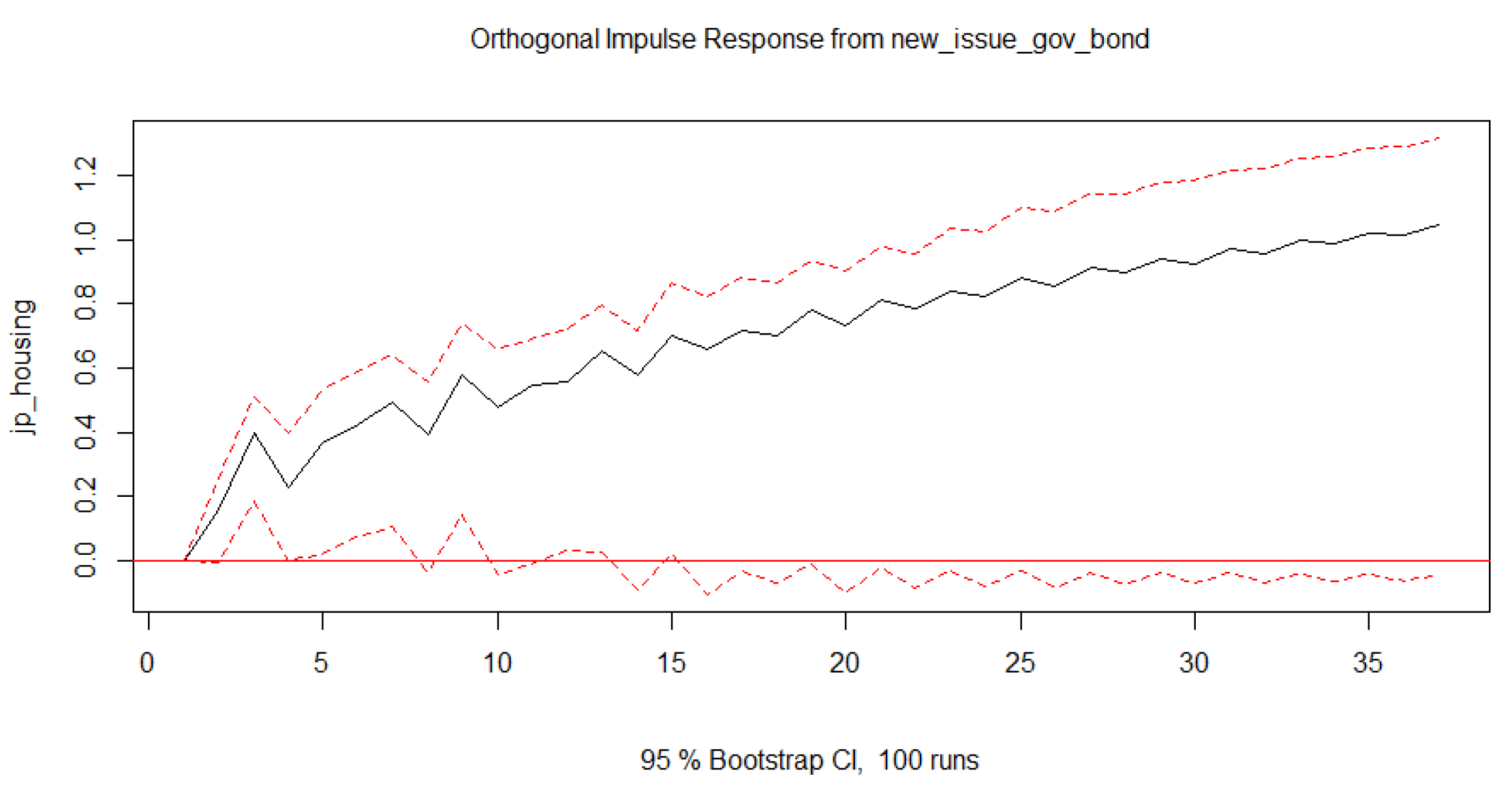
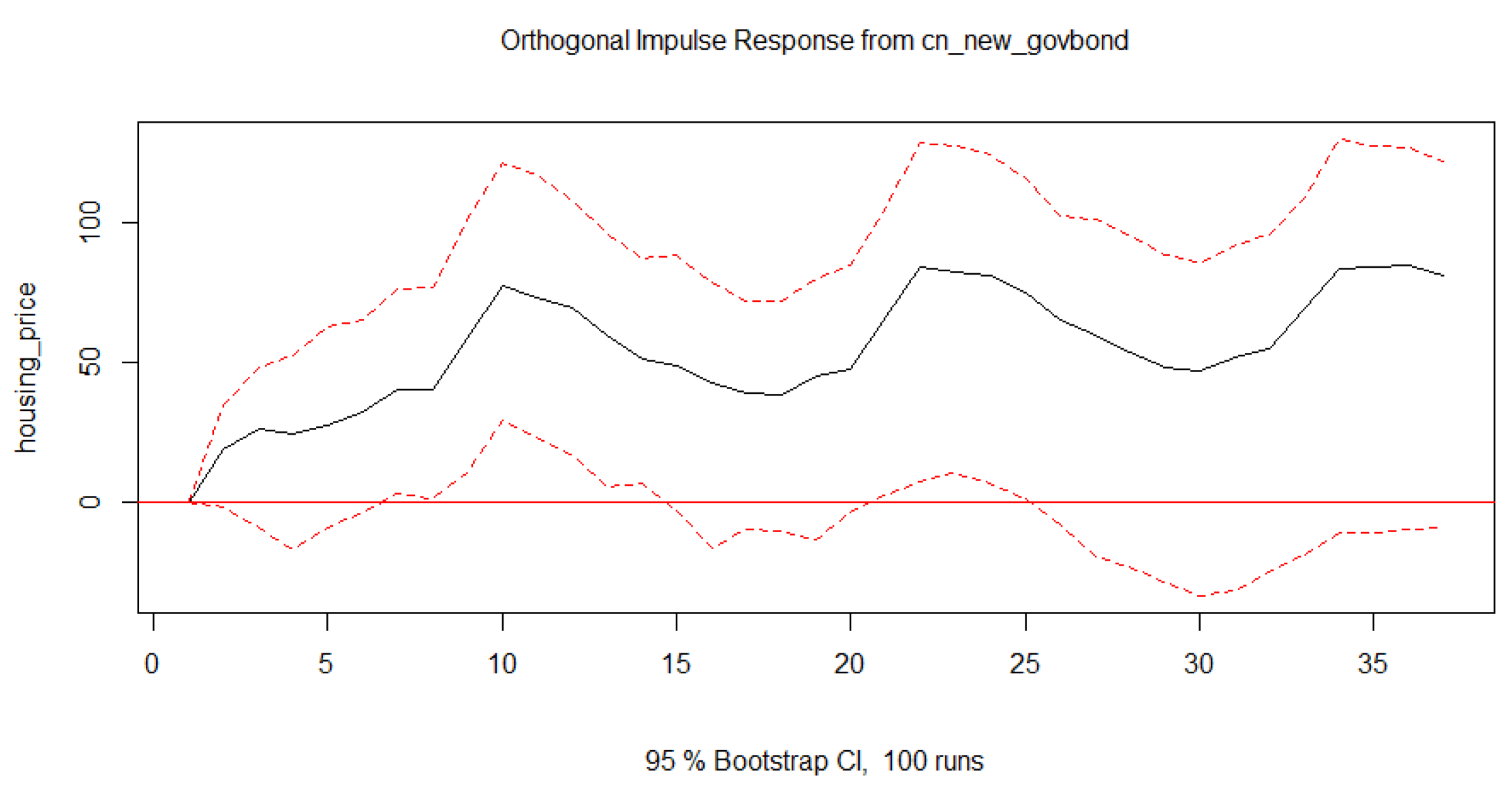
Current academic research primarily focuses on the impact of interest rates and the yield curve on housing prices, while studies investigating the effects of open market operations and new issuances of government bonds on housing prices are relatively scarce. Existing literature that addresses the influence of open market operations on asset prices, such as housing prices and exchange rates, generally does so within the broader framework of monetary policy. Specifically, This article will explore how the quantity of newly issued government bonds affects housing prices, providing insights to help central banks manage financial risks and maintain economic stability more effectively.

4.3.1. Data Table

Table 7. ADF Test Results for JP_housing and New_issue_gov_bond.

Variable	Dickey-Fuller	Lag Order	p-value
JP_housing	-2.1326	5	0.5206
New_issue_gov_bond	-2.2493	5	0.4718

The ADF test results indicate that both JP_housing and New_issue_gov_bond are likely non-stationary. For JP_housing, the Dickey-Fuller statistic is -2.1326 with a p-value of 0.5206, which is well above the 0.05 significance level, indicating that we cannot reject the null hypothesis of a unit root. This suggests that the housing price series exhibits characteristics of a random walk and may have trends or volatility. Similarly, for New_issue_gov_bond, the Dickey-Fuller statistic is -2.2493 with a p-value of 0.4718, also failing to reject the null hypothesis of non-stationarity. These results imply that both time series may need to be differenced or otherwise transformed to achieve stationarity before further analysis can be performed reliably. Given that both variables are non-stationary, it is appropriate to conduct a Johansen cointegration analysis

Table 8. Johansen Cointegration Test Results (Trace Statistic with Linear Trend).

Hypothesis	Test Statistic	15%	10%	5%	1%
$r \leq 1$	0.53	4.82	6.50	8.18	11.65
$r = 0$	15.01	14.82	15.66	17.95	23.52

The table presents the Johansen cointegration test results based on the Trace statistic, which evaluates whether there is a cointegration relationship among the time series. For the hypothesis

r \leq 1

, the Trace statistic is 0.53, which is significantly lower than all critical values at the 15%, 10%, 5%, and 1% significance levels (4.82, 6.50, 8.18, and 11.65, respectively). This indicates that the null hypothesis of no additional cointegration relationship cannot be rejected, suggesting that the data does not support the existence of more than one cointegration relationship under this setting. For the hypothesis

r = 0

, the Trace statistic is 15.01, which falls slightly below the 10% critical value (15.66) but exceeds the 15% critical value (14.82). This implies that at the 15% significance level, the null hypothesis of no cointegration can be rejected, suggesting a potential cointegration relationship. However, at more stringent significance levels (10%, 5%, or 1%), there is insufficient evidence to support this conclusion. It is important to note that the 15% critical values in the table were estimated using linear interpolation.

Table 9. Regression Results for jp_housing.d.

Coefficient	Estimate	Std. Error	t value
ect1	-0.00897	0.00286	-3.141 **
constant	-2.57761	0.88980	-2.897 **
jp_housing.dl1	-0.42266	0.07607	-5.556 ***
new_issue_gov_bond.dl1	0.00032	0.00017	1.891 .
jp_housing.dl2	-0.12502	0.08195	-1.526
new_issue_gov_bond.dl2	0.00080	0.00020	4.067 ***
jp_housing.dl3	-0.22129	0.08251	-2.682 **
new_issue_gov_bond.dl3	0.00038	0.00021	1.781 .
⋮	⋮	⋮	⋮
new_issue_gov_bond.dl7	0.00036	0.00019	1.953 .

8cm Multiple R-squared: 0.3864, Adjusted R-squared: 0.3290

The regression results for jp_housing.d show several significant factors influencing housing price changes in Japan. The error correction term (ect1) is statistically significant with a negative coefficient (-0.00897), indicating that deviations from the long-term equilibrium are corrected over time. The lagged value of housing prices (jp_housing.dl1) also shows a significant negative effect, suggesting that past increases in housing prices are associated with decreases in the current period, possibly reflecting a correction mechanism in the housing market.

The coefficients for new_issue_gov_bond lag terms indicate mixed effects. For example, new_issue_gov_bond.dl2 is highly significant (p < 0.001), suggesting that an increase in newly issued government bonds may have a positive impact on housing prices with a lag. Other lags of new_issue_gov_bond show varying levels of significance, implying that the effect of new bond issuances on the housing market may not be consistent across different time lags.

Overall, the model explains about 38.6% of the variance in housing price changes, indicating a moderate fit. The significant F-statistic suggests that the model as a whole is statistically significant. Now, we can build a equation.

\begin{matrix} {jp_housing . d}_{t} = & β_{1} {ect 1}_{t} + β_{2} constant + β_{3} {jp_housing . dl 1}_{t - 1} + β_{4} {new_issue_gov_band . dl 1}_{t - 1} \\ + β_{5} {jp_housing . dl 2}_{t - 2} + β_{6} {new_issue_gov_band . dl 2}_{t - 2} + \dots \\ + β_{15} {jp_housing . dl 7}_{t - 7} + β_{16} {new_issue_gov_band . dl 7}_{t - 7} + ϵ_{t} \end{matrix}

(7)

Where

${jp_housing . d}_{t}$ : The change in housing prices at time t.
${ect 1}_{t}$ : The error correction term, indicating deviations from long-term equilibrium.
constant: A constant term capturing fixed effects in the model.
${jp_housing . dl 1}_{t - 1}, \dots, {jp_housing . dl 7}_{t - 7}$ : The lagged values of housing price changes, representing the past values up to seven periods.
${new_issue_gov_band . dl 1}_{t - 1}, \dots, {new_issue_gov_band . dl 7}_{t - 7}$ : The lagged values of new government bond issuances, indicating the impact of government bond issuance over the past seven periods.
$ϵ_{t}$ : The error term, capturing the unexplained variation in the model.

For Chinese scenario:

Table 10. ADF Test Results for Housing Price and CN_New_Govbond.

Variable	Dickey-Fuller	Lag Order	p-value
Housing Price	-2.8278	6	0.2274
CN_New_Govbond	-1.2624	6	0.8876

The table presents the results of the Augmented Dickey-Fuller (ADF) test for two variables: housing prices and CN_New_Govbond (Chinese new government bond issuances). The ADF test checks whether a time series is stationary or not. For housing prices, the Dickey-Fuller statistic is -2.8278 with a p-value of 0.2274, indicating that we cannot reject the null hypothesis of a unit root, suggesting the series is likely non-stationary. Similarly, for CN_New_Govbond, the Dickey-Fuller statistic is -1.2624 with a p-value of 0.8876, also failing to reject the null hypothesis, indicating that this series is likely non-stationary as well.Since both variables are non-stationary, it is appropriate to conduct a Johansen cointegration test to determine whether there exists a long-term equilibrium relationship between them. The Johansen test will help identify any cointegrating vectors that may suggest a stable relationship over the long run despite the individual series being non-stationary.

Table 11. Johansen Cointegration Test Results (Trace Statistic Without Linear Trend and Constant).

Hypothesis	Test Statistic	10%	5%	1%
$r \leq 1$	11.29	7.52	9.24	12.97
$r = 0$	44.58	17.85	19.96	24.60

The Johansen cointegration test results provide evidence of a cointegration relationship between the variables. The trace statistic, without considering a linear trend and constant, indicates that for the hypothesis

r \leq 1

, the test statistic is 11.29, which exceeds the 5% critical value of 9.24. This allows us to reject the null hypothesis of at most one cointegration relationship, suggesting the existence of at least one cointegrating vector. Additionally, for the hypothesis

r = 0

, the test statistic is 44.58, which is well above the critical values at the 10%, 5%, and 1% levels (17.85, 19.96, and 24.60, respectively). This confirms the presence of a cointegration relationship. Overall, these findings imply that the variables exhibit a stable long-term equilibrium relationship, moving together over time even though they may be individually non-stationary. So, now we can build VECM model.

Table 12. Regression Results for Housing Price Changes.

Coefficient	Estimate	Std. Error	t value
ect1	-0.00129	0.00128	-1.007
housing_price.dl1	-0.03682	0.05081	-0.725
cn_new_govbond.dl1	0.00018	0.00009	1.933 .
housing_price.dl2	-0.15202	0.05029	-3.023 **
cn_new_govbond.dl2	0.00021	0.00012	1.824 .
⋮	⋮	⋮	⋮
housing_price.dl12	0.5343	0.05407	9.882 ***
cn_new_govbond.dl12	0.00022	0.00010	2.229 *

8cm Multiple R-squared: 0.412, Adjusted R-squared: 0.3613

The regression results show that some lagged variables have a significant impact on housing price changes. The error correction term (ect1) is not statistically significant, indicating that deviations from the long-term equilibrium may not have a strong correction effect. Some lagged terms of housing prices (e.g., housing_price.dl2 and housing_price.dl12) are significant, suggesting that past values influence current changes.

Lagged terms of the new government bond issuances (e.g., cn_new_govbond.dl12) are also significant, implying that the issuance of new bonds can affect housing prices. The model explains about 41.2% of the variation in housing prices, with an overall significant F-statistic, indicating a good fit for the data.

\begin{matrix} {housing_price . d}_{t} = & β_{1} {ect 1}_{t} + β_{2} {housing_price . dl 1}_{t - 1} + β_{3} {cn_new_govbond . dl 1}_{t - 1} \\ + β_{4} {housing_price . dl 2}_{t - 2} + β_{5} {cn_new_govbond . dl 2}_{t - 2} + \dots \\ + β_{24} {housing_price . dl 12}_{t - 12} + β_{25} {cn_new_govbond . dl 12}_{t - 12} + ϵ_{t} \end{matrix}

(8)

Where:

${housing_price . d}_{t}$ : Change in housing prices at time t.
${ect 1}_{t}$ : Error correction term, representing deviations from the long-term equilibrium.
${housing_price . dl 1}_{t - 1}, \dots, {housing_price . dl 2}_{t - 12}$ : Lagged values of housing price changes, capturing the impact of past housing price variations.
${cn_new_govbond . dl 1}_{t - 1}, \dots, {cn_new_govbond . dl 12}_{t - 12}$ : Lagged values of new government bond issuances, reflecting the influence of bond issuance on housing prices.
$ϵ_{t}$ : Error term, representing unexplained variations in the model.

4.3.2. Figures

We can start to build VECM model and plot graph:

We can see Figure 7 shows the impulse response of Japan’s housing market to a shock in newly issued government bonds. The response starts with a small positive effect, gradually increasing over time and becoming more pronounced after 10 periods. This suggests that newly issued government bonds have a delayed impact on the housing market, potentially boosting housing prices as the market reacts to increased government spending or liquidity.

Figure 8 illustrates the impulse response of China’s housing market to a similar shock in newly issued government bonds. Unlike Japan, the initial response in China is more volatile, with significant fluctuations in the early periods. The effect stabilizes after approximately 15 periods, with an overall upward trend.

5. Robustness Checks

Table 13. VECM Model Results for Early and Late Subsamples (JP_housing.d Equation).

Variable	Early Estimate	Early p-value	Late Estimate	Late p-value
Error correction term (ect1)	-1.0830	0.0001***	-0.3300	0.0018**
JP_rate lag 1 (JP_rate.dl1)	3.6908	0.5267	12.6900	0.1101
JP_housing lag 1 (JP_housing.dl1)	-0.7755	0.00001***	-0.3950	0.00002***
JP_rate lag 2 (JP_rate.dl2)	3.4453	0.5329	-12.9519	0.1063
JP_housing lag 2 (JP_housing.dl2)	-0.2967	0.1074	-0.0312	0.7410
JP_housing lag 3 (JP_housing.dl3)	-0.2226	0.2224	-0.2491	0.0104*

Significance levels: * p <0.05, ** p <0.01, *** p <0.001

The VECM model shows partial robustness, with the error correction term (ect1) and JP_housing lag 1 significant in both subsamples, indicating consistent long-term adjustment and inertia effects in housing prices. However, the varying significance of other lags, such as JP_housing lag 3 being significant only in the late subsample, suggests potential changes in market dynamics over time, affecting the model’s stability.

Table 14. VECM Model Results for Early and Late Subsamples (CN_housing.d Equation).

Variable	Early Estimate	Early p-value	Late Estimate	Late p-value
Error correction term (ect1)	-38.16	0.197	-81.88	0.045*
SHIBOR lag 1	57.94	0.273	12.13	0.792
CN_housing lag 1	-0.08	0.519	0.01	0.887
SHIBOR lag 2	-31.30	0.555	-22.59	0.638
CN_housing lag 2	-0.37	0.005**	-0.18	0.050 .
...	...	...	...	...

Significance levels: * p <0.05, ** p <0.01, *** p <0.001

The robustness of the VECM model is assessed through subsample analysis, comparing early and late periods. The error correction term (ect1) being significant only in the late subsample suggests that the adjustment towards long-term equilibrium strengthens over time, indicating changes in market behavior. The consistent significance of CN_housing lag 2 across both subsamples supports the model’s robustness, as it demonstrates a persistent short-term effect. However, variations in the magnitude and significance of other coefficients, such as the decreasing impact of CN_housing lag 2, indicate that the model’s stability may vary depending on the time period, pointing to partial robustness.

Table 15. VECM Model Results for Early and Late Subsamples (JP_housing.d Equation).

Variable	Early Estimate	Early p-value	Late Estimate	Late p-value
Error correction term (ect1)	-4.84e-05	0.0005***	4.04e-04	1.98e-05***
New_issue_gov_bond lag 1	-1.09e-04	0.6284	2.32e-04	0.2657
JP_housing lag 1	-0.71	2.24e-05***	-0.44	3.26e-06***
New_issue_gov_bond lag 2	4.38e-04	0.0578 .	9.11e-04	0.0004***
JP_housing lag 2	-0.25	0.1434	-0.14	0.1325
JP_housing lag 3	-0.25	0.1130	-0.28	0.0028**
...	...	...	...	...

Significance levels: * p <0.05, ** p <0.01, *** p <0.001

The VECM results show differences in the adjustment dynamics for JP_housing between the early and late subsamples. The error correction term (ect1) is significant in both subsamples but changes signs, indicating shifts in the adjustment process over time. The consistent significance of JP_housing lag 1 in both periods suggests a robust short-term effect, while the increased significance of higher lags (e.g., JP_housing lag 3) in the late subsample implies evolving market dynamics. Overall, while the model exhibits some consistency across periods (such as the significance of JP_housing lag 1), the changes in the error correction term and higher-order lags reflect potential shifts in market dynamics. This indicates that the model demonstrates partial robustness, but certain dynamic characteristics may affect its stability over time.

Table 16. VECM Model Results for Early and Late Subsamples (CN_new_govbond.d Equation).

Variable	Early Estimate	Early p-value	Late Estimate	Late p-value
Error correction term (ect1)	-0.67315	3.19e-06***	-0.12449	0.0333*
CN_new_govbond lag 1	-0.91807	<2e-16***	-0.49365	6.26e-07***
Housing_price lag 1	-14.00163	0.6509	-43.73220	0.5095
CN_new_govbond lag 2	-0.92062	3.81e-16***	-0.30517	0.0040**
Housing_price lag 2	-18.76892	0.5453	-1.26694	0.9847
CN_new_govbond lag 3	-0.88209	1.91e-11***	-0.24048	0.0284*
Housing_price lag 4	52.98381	0.0861 .	5.94665	0.9272
...	...	...	...	...

Significance levels: * p <0.05, ** p <0.01, *** p <0.001

The VECM results for the early and late subsamples show some differences in the adjustment dynamics of CN_new_govbond. The error correction term (ect1) is significant in both periods, indicating a consistent adjustment towards the long-term equilibrium, although the effect weakens in the later subsample. The consistent significance of CN_new_govbond lag 1 and lag 2 across both subsamples supports the model’s robustness, suggesting a persistent short-term effect. However, the reduced significance of lag 3 and the changing signs of coefficients for Housing_price lags imply potential changes in market behavior over time, indicating that while the model demonstrates partial robustness, some variations may affect its stability.

6. Conclusions

The study examines the dynamic relationships between macroeconomic policies and household wealth, with a focus on housing prices in China and Japan. By utilizing advanced econometric techniques such as VAR, VECM, and impulse response analysis, the research finds that both monetary and fiscal policies significantly impact housing market dynamics. Aggressive monetary policies, such as interest rate cuts and reserve requirement reductions, tend to stimulate housing demand and increase prices. Similarly, the issuance of new government bonds positively influences housing prices by injecting liquidity into the economy. However, the effects differ across countries; for example, Japan’s housing market shows a more persistent response to interest rate shocks compared to China’s. These findings highlight the importance of accounting for country-specific factors and policy effects when analyzing the housing market and designing economic interventions.

References

Pyhrr, S.; Roulac, S.; Born, W. Real estate cycles and their strategic implications for investors and portfolio managers in the global economy. Journal of Real Estate Research 1999, 18, 7–68. [Google Scholar] [CrossRef]
Kaiser, R. The long cycle in real estate. Journal of Real Estate Research 1997, 14, 233–257. [Google Scholar] [CrossRef]
Ewing, B.T.; Payne, J.E. The response of real estate investment trust returns to macroeconomic shocks. Journal of Business Research 2005, 58, 293–300. [Google Scholar] [CrossRef]
Nguyen, M.L.T.; Bui, T.N.; Nguyen, T.Q. Relationships between real estate markets and economic growth in Vietnam. The Journal of Asian Finance, Economics and Business 2019, 6, 121–128. [Google Scholar] [CrossRef]
Cellmer, R.; Bełej, M.; Cichulska, A. Identification of cause-and-effect relationships in the real estate market using the VAR model and the Granger test. Real Estate Management and Valuation 2019, 27, 85–95. [Google Scholar] [CrossRef]
Ju, F.; Lin, H.; Zhou, J. Regional differences in the impact of land transfer revenue and local fiscal expenditure on housing prices in China. Theory and Practice of Finance and Economics 2013, 1, 77–81. [Google Scholar]
Sims, C.A. Macroeconomics and reality. Econometrica: Journal of the Econometric Society, 1980; 1–48. [Google Scholar]
Nakajima, J. Time-varying parameter VAR model with stochastic volatility: An overview of methodology and empirical applications 2011.
Jacobson, T.; others. A VAR model for monetary policy analysis in a small open economy. Sveriges Riksbank Working Paper Series 1999. [Google Scholar]
Wang, Y.; Haili, D.; Cuiqing, C. The relationship between household leverage, real estate, and consumption growth in China. Finance and Economy 2021. [Google Scholar]
Meng, P.; Fei, L.; Gao, C.; Wu, L.; Sun, X. The impact of reserve requirement ratio changes on the liquidity of commercial banks in China: An empirical study based on the VAR model and impulse response function. Modern Finance 2024, 3, 26–32, CNKI:SUN:LCJR.0.2024-03-004. [Google Scholar]

Figure 7. Impulse Response of Japan housing to Newly issued government bond

Figure 8. Impulse Response of China housing to Newly issued government bond

Disclaimer/Publisher’s Note: The statements, opinions and data contained in all publications are solely those of the individual author(s) and contributor(s) and not of MDPI and/or the editor(s). MDPI and/or the editor(s) disclaim responsibility for any injury to people or property resulting from any ideas, methods, instructions or products referred to in the content.

© 2024 by the authors. Licensee MDPI, Basel, Switzerland. This article is an open access article distributed under the terms and conditions of the Creative Commons Attribution (CC BY) license (http://creativecommons.org/licenses/by/4.0/).

Copyright: This open access article is published under a Creative Commons CC BY 4.0 license, which permit the free download, distribution, and reuse, provided that the author and preprint are cited in any reuse.

MDPI Initiatives

Important Links

Choose an area of interest and we will send you notifications of new preprints at your preferred frequency.

Disclaimer

Aggressive Monetary and Fiscal Policy Impact on Household Wealth: A Comparative Analysis of China and Japan

Abstract

1. Introduction

2. Literature Review

3. Research Methodology

4. Housing

4.1. Cyclical Phenomenon of Housing Price

4.2. VAR model of Housing Price for Interest rate ( Δ Trend)

4.2.1. Data Table

4.2.2. Figures

4.3. VAR Model of Housing Price for New Issued Government Bond ( Δ Trend)

4.3.1. Data Table

4.3.2. Figures

5. Robustness Checks

6. Conclusions

References

MDPI Initiatives

Important Links

Subscribe

4.2. VAR model of Housing Price for Interest rate ( $Δ$ Trend)

4.3. VAR Model of Housing Price for New Issued Government Bond ( $Δ$ Trend)