1. Introduction
Dynamic response prediction of structural systems plays a pivotal role in both the design and evaluation of individual buildings and the reliability assessment of infrastructure and large urban areas [
1]. Conventionally, this process entails the creation of numerical models for dynamic systems, with response prediction facilitated by numerical differential equation solvers like the Newmark-β method [
2]. The finite element method (FEM) stands out as a prominent technique in this domain, extensively employed across various engineering disciplines such as civil, mechanical, and aeronautical engineering [
3]. Despite significant advancements in computational capabilities, the escalating complexity of numerical models poses formidable challenges, especially in dealing with large-scale engineering problems characterized by nonlinear hysteretic behaviors under dynamic loads [
4]. The computational burden becomes particularly onerous when addressing optimization tasks and handling stochastic uncertainties associated with external loads. Techniques like Monte Carlo simulations and incremental dynamic analysis (IDA) are indispensable in accounting for these uncertainties, but they significantly augment the computational cost [
5].
When assessing structures under seismic excitation, it is crucial to account for the variability in frequency content across different recorded earthquakes [
6]. Each earthquake has unique characteristics, and relying on a single record may not capture the full range of possible seismic responses. Therefore, in order to perform a thorough evaluation, it is advisable to use a large set of records, for instance 80 different earthquake recordings [
2]. Additionally, to understand the structure’s performance under increasing seismic demand, the intensity of each earthquake record should be scaled multiple times, for example, ten intensity levels per record. This process helps capture how a structure behaves under a wide spectrum of seismic intensities. For instance, consider an earthquake record that lasts 50 seconds and is sampled at a time step of 0.005 seconds. This results in 10,000 data points for that single record. When performing an (IDA) using 80 earthquake records and scaling each record 10 times, the total number of data points grows significantly. Specifically, the analysis will involve 80 × 10 × 10,000 = 8,000,000 data points[
7].
In addition to the large number of data points generated from the earthquake records, the structural models themselves involve complex equations that include large matrices representing stiffness, mass, damping, and other dynamic properties [
8]. These matrices are essential for accurately capturing the behavior of structures under seismic loads. For example, the stiffness matrix defines how resistant a structure is to deformation, while the mass matrix accounts for how inertia affects the structure’s response to motion. The damping matrix, meanwhile, represents energy dissipation mechanisms within the structure. This challenge persists despite the availability of high-performance computing clusters or facilities. Consequently, the quest for efficient computational methodologies to tackle these complexities remains a pressing concern in the realm of structural dynamic analysis and design [
9].
In response to the computational challenges posed by complex engineering simulations, researchers have delved into the realm of metamodeling as a means to alleviate the computational burden [
10]. Metamodels serve as reduced-fidelity surrogate models of high-fidelity simulations, aiming to capture the input-output relationships of systems while significantly reducing computational costs [
10]. Traditionally, techniques such as regression and response surface methodology (RSM) have been prevalent in metamodeling, relying on polynomial least-square fitting [
11]. However, the simplicity of these methods and their dependence on second-order polynomials often lead to insufficient accuracy, particularly in capturing highly nonlinear system behaviors [
11]. To address these limitations, alternative metamodeling approaches have emerged, including Kriging, support vector machine, and polynomial chaos expansions, among others [
12,
13,
14]. These methods offer promising avenues for uncertainty quantification and have found applications in various engineering domains.
However, the calibration of high-fidelity models, especially those with numerous parameters, demands significant computational resources [
15]. To mitigate this challenge, model order reduction techniques have been developed [
15]. These techniques enable the creation of reduced-fidelity metamodels that approximate the behavior of complex systems while substantially reducing computational costs. Despite these advancements, current methodologies often struggle to address highly nonlinear structures under non-stationary conditions [
15]. This limitation underscores the ongoing need for innovative approaches to metamodeling, particularly in the context of complex engineering systems subjected to dynamic loads and nonlinear behaviors. Efforts to bridge this gap are vital for advancing the efficiency and accuracy of computational simulations in engineering design and analysis. To extend the applicability and accuracy of dynamic response predictions, ongoing research endeavors are exploring innovative methodologies. These include leveraging machine learning (ML) techniques to refine model updating processes and enhance the predictive capabilities of numerical simulations.
Zhanga et al. [
15] have developed an approach to metamodeling nonlinear structural systems with limited data by integrating partial physics knowledge into deep long short-term memory (LSTM) networks. Their framework ensures precise model training by incorporating physics constraints into the loss function, effectively capturing system nonlinearity. Tailored for dynamic structures, the framework considers equations of motion, state dependence, and hysteretic constitutive relationships. The embedded physics mitigate overfitting, reduce dependency on extensive training datasets, and enhance model robustness, surpassing that of traditional data-driven neural networks. Eshkevari et al. [
16] present a physics-informed recurrent neural network (RNN) model designed to predict the dynamics of multi-degree-of-freedom systems subjected to diverse ground motions. The model predicts displacement, velocity, acceleration, and internal forces, outperforming existing models with improved predictive accuracy and fewer parameters. Inspired by differential equation solvers, the recurrent block architecture aims for more generalized solutions. Innovative training techniques such as hard sampling, trajectory loss function, and trust-region optimization expedite learning with limited datasets. Zhang et al. [
17] present a novel approach using a physics-guided convolutional neural network (PhyCNN) for data-driven modeling of structural seismic responses. Their method integrates physics constraints into deep learning models, allowing for accurate prediction of structural responses with limited seismic datasets. Numerical simulations and experiments confirm PhyCNN’s acceptable performance in predicting seismic responses.
Xu et al. [
18] introduce an innovative physics-informed ML approach leveraging Convolutional Neural Networks (CNNs) to accurately reconstruct both dynamic and static displacements of plate-beam composite structures. Integrating past acceleration-related physics knowledge into the deep learning framework is the core concept. To improve physics-based training efficiency, a dual-branch network architecture is developed to extract extensive details from inputs. Multi-task weights are adjusted using carefully selected scales and punishment factors. A comparison of their suggested methodology with computer simulations and empirical validations in the statics and structural dynamics domains demonstrates its superior performance. Incorporating acceleration data improves the trained model’s robustness for more accurate displacement predictions while also drastically lowering measurement costs. Hu et al. [
19] presented a new neural network, merging physics-informed neural networks with model-based transfer learning, for better seismic response predictions with limited data. Integrating physics knowledge, represented by a new solver, enhances the network’s ability to capture structural nonlinearities. Model-based transfer learning improves generalization by transferring features from a source to target buildings. Their model outperforms data-driven networks in predicting seismic responses across target buildings from numerical models to physical shaking table tests.
There are persistent challenges in training a dependable deep learning model for estimating the response of nonlinear structures subjected to seismic excitation. Notably, the process of solving partial differential equations (PDEs) or governing equations within Physics-Informed Neural Networks (PINNs) often entails iterative numerical methods, which incur significant computational costs, particularly for large-scale structural configurations. Consequently, this computational overhead can impede real-time applications and the execution of extensive simulations crucial for comprehensive seismic risk evaluation. Moreover, the application of physics-informed neural networks to intricate and inherently chaotic systems, such as those governed by soil-structure interaction or characterized by rocking behavior [
20], remains arduous due to the inherent limitations in handling the heightened complexity of the data, surpassing the capabilities of current physics-guided models [
19]. In addition, while previous studies introduced techniques that excel in generating intricate reconstructions of the time-history response based on their training datasets, they primarily cater to relatively straightforward structures. These structures typically include single-degree-of-freedom systems, shear-type multi-degree-of-freedom structures with hysteresis modeled numerically, or low-rise buildings with fewer than three stories. However, their applicability may be limited when it comes to capturing the intricate behaviors arising from material and geometric nonlinearities across a spectrum of building heights.
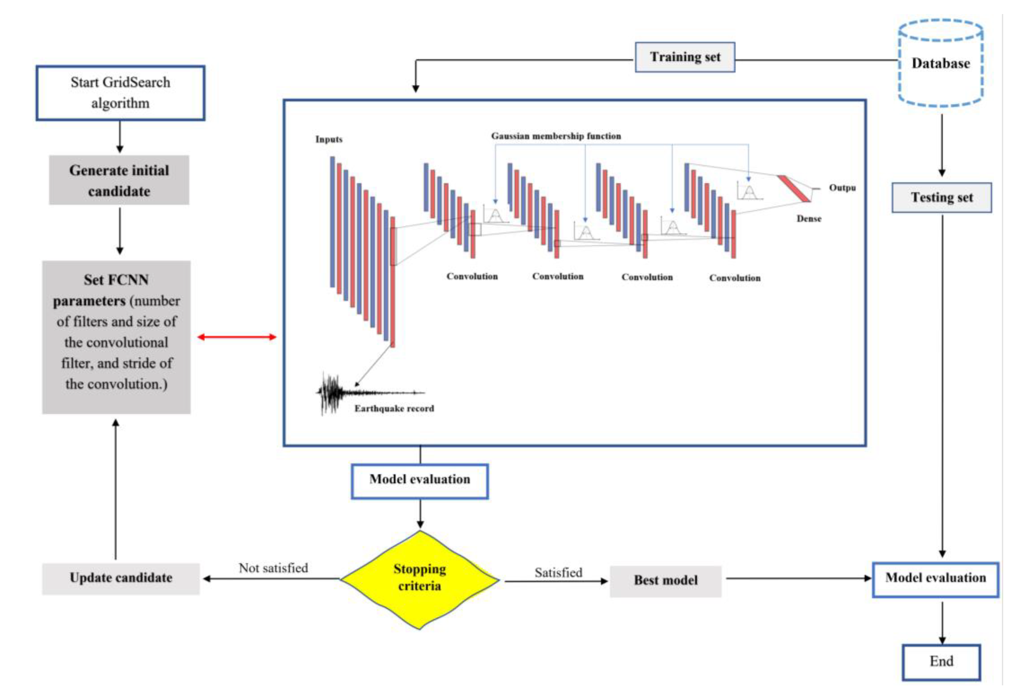
In this study, a novel approach is proposed by integrating fuzzy logic principles into a CNN framework, termed FuzzyCNN, to effectively model and predict the dynamic behavior of soil-structure systems under seismic excitations. The FuzzyCNN model is designed to handle the uncertainties and complexities inherent in such systems, leveraging the interpretability of fuzzy logic combined with the robust feature extraction capabilities of CNNs. The primary objectives of this research are to develop a FuzzyCNN model capable of accurately predicting the responses of structures subjected to earthquake loads and to compare its performance against traditional physics-informed CNN (PhyCNN) models. Specifically, we aim to address the following research questions: How does the integration of fuzzy logic into a CNN affect the model’s accuracy and robustness? Can the FuzzyCNN model outperform existing PhyCNN models in terms of prediction accuracy and handling of uncertainties? The remainder of this paper is structured as follows:
Section 2 details the methodology, including the development of the FuzzyCNN model and the numerical techniques employed for its validation.
Section 3 presents the results and discussion, providing a comparative analysis of the FuzzyCNN and PhyCNN models based on various performance metrics. Finally,
Section 4 concludes the paper, highlighting the key findings and potential future research directions.
2. Problem Definition
Dynamic equilibrium equations considering soil-structure interaction and seismic excitation typically involve accounting for the behavior of both the structure and the underlying soil medium. These equations describe the balance of forces acting on the system while considering the dynamic response to seismic loading. They can be expressed in matrix form as [
21]:
where
and
represent the mass and damping matrices of the system, respectively.
is the stiffness matrix of the structure,
is the interaction stiffness matrix between the structure and the soil,
denotes the displacement vector of the structure, and
denotes the relative displacement vector between the structure and the soil.
and
denote the acceleration and velocity vectors, while
signifies the vector of reactions from the time-dependent springs and dampers that have replaced the soil or the external force vector due to seismic excitation. It’s possible to merge
and
into a single term, representing the total stiffness effect on the system. This combined stiffness term accounts for both the intrinsic stiffness of the structure and the stiffness due to interaction with the soil. It simplifies the dynamic equilibrium equations for a system subjected to seismic excitation, depicted in
Figure 1 [
22]:
where
represents the total stiffness matrix, combining both the structural stiffness and the interaction stiffness.
The dimensions of these matrices and vectors correspond to the total degrees of freedom in the system. Notably, the coefficients of the springs and dampers are analogous to the support’s flexibility concerning vibration frequency. Hence, a transformation from the time domain to the frequency domain facilitates an easier solution of Equation (1). This transformation can be achieved through the use of the Fourier transform (
), as depicted in Equation (3) [
23]:
Moreover, leveraging the properties of the Fourier transform, Equation (4) emerges [
24]:
where
represents the dynamic stiffness matrix of the structure. In addition, Rayleigh damping is commonly assumed, where damping is proportional to both velocity and stiffness, formulated as [
25]:
Here,
and
are constant coefficients derived from the system’s dynamic characteristics. In the domain of structural-soil interaction, a mixed stiffness matrix is employed in the frequency domain, comprising both real and imaginary components [
25,
26]. This mixed stiffness matrix signifies a phase discrepancy between the applied load and the resulting reaction, indicating a delay in the reaction relative to the applied load due to system damping. Upon comparing equations (1) and (3), it becomes apparent that solving the dynamic equilibrium equation of the system in the frequency domain, i.e., is notably more straightforward using fundamental principles of algebraic equations [
25,
26]. However, a significant challenge lies within these equations: besides the unknown displacements
, the Fourier transform of the reaction vector
is also unknown, as
represents the forces acting on the flexible support, inherently ambiguous. Consequently, the system presents one equation with two unknowns, resulting in an indeterminate problem [
25,
26].
4. Results and Discussion
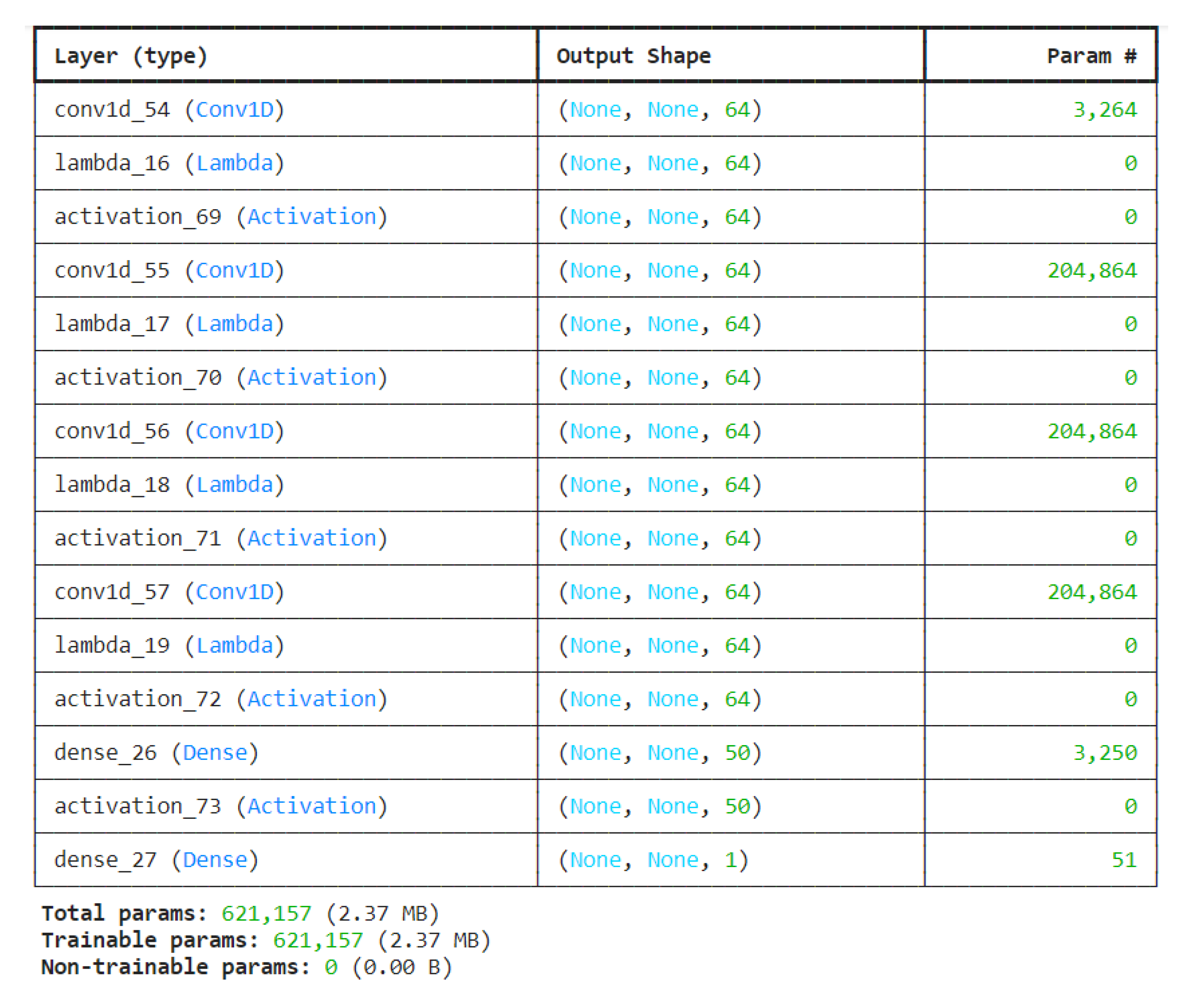
Figure 4 and
Figure 5 show the architecture of the FuzzyCNN and PhyCNN models. The number of parameters in a neural network model is a critical factor that can affect the model’s complexity, training time, and risk of overfitting. The proposed model (FuzzyCNN) has 621,157 parameters, while PhyCNN has 828,571 parameters. The PhyCNN model has approximately 207,414 more parameters than the FuzzyCNN model. This larger parameter count suggests that PhyCNN incurs increased computational costs and carries a potentially higher risk of overfitting, particularly when dealing with limited data [
36].
Figure 6 illustrates the predicted behavior of the SDOF structural system using the FuzzyCNN model. The plot represents the displacement of the structural response. The figure demonstrates the model’s ability to capture the nuanced responses of an SDOF system under various conditions.
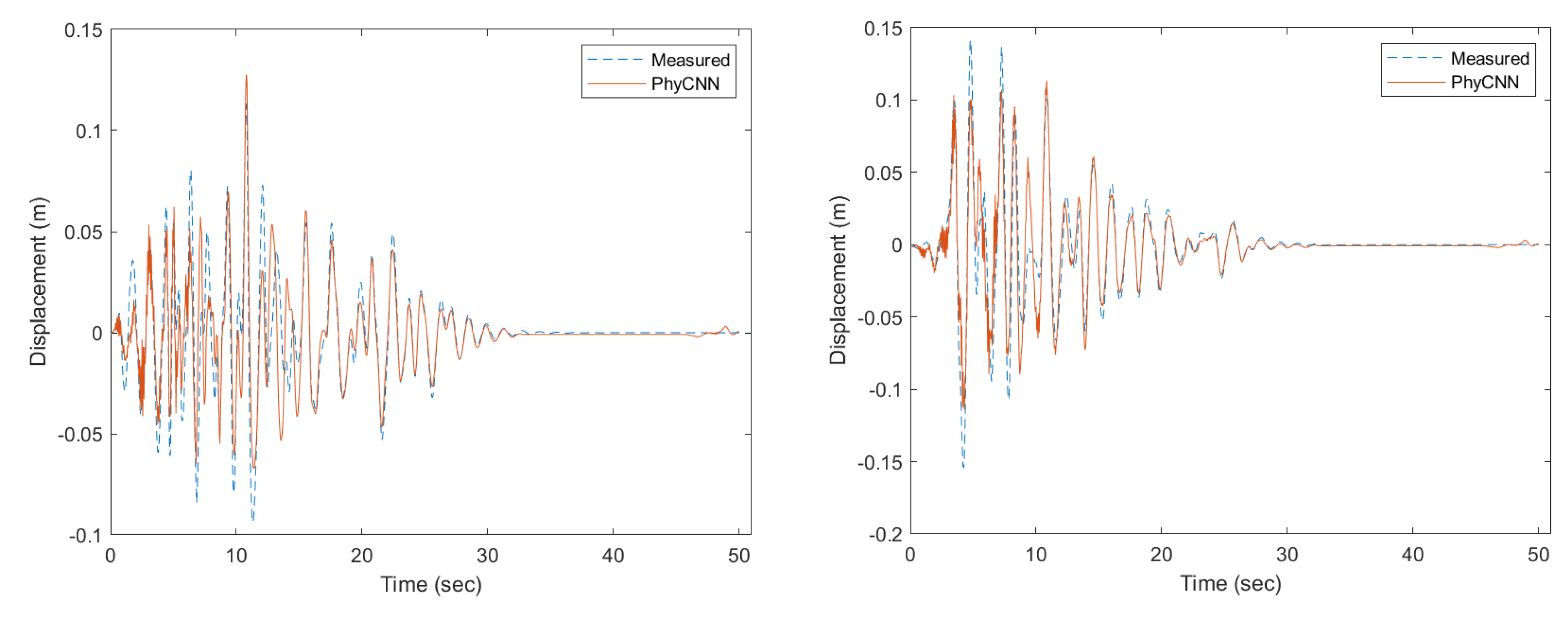
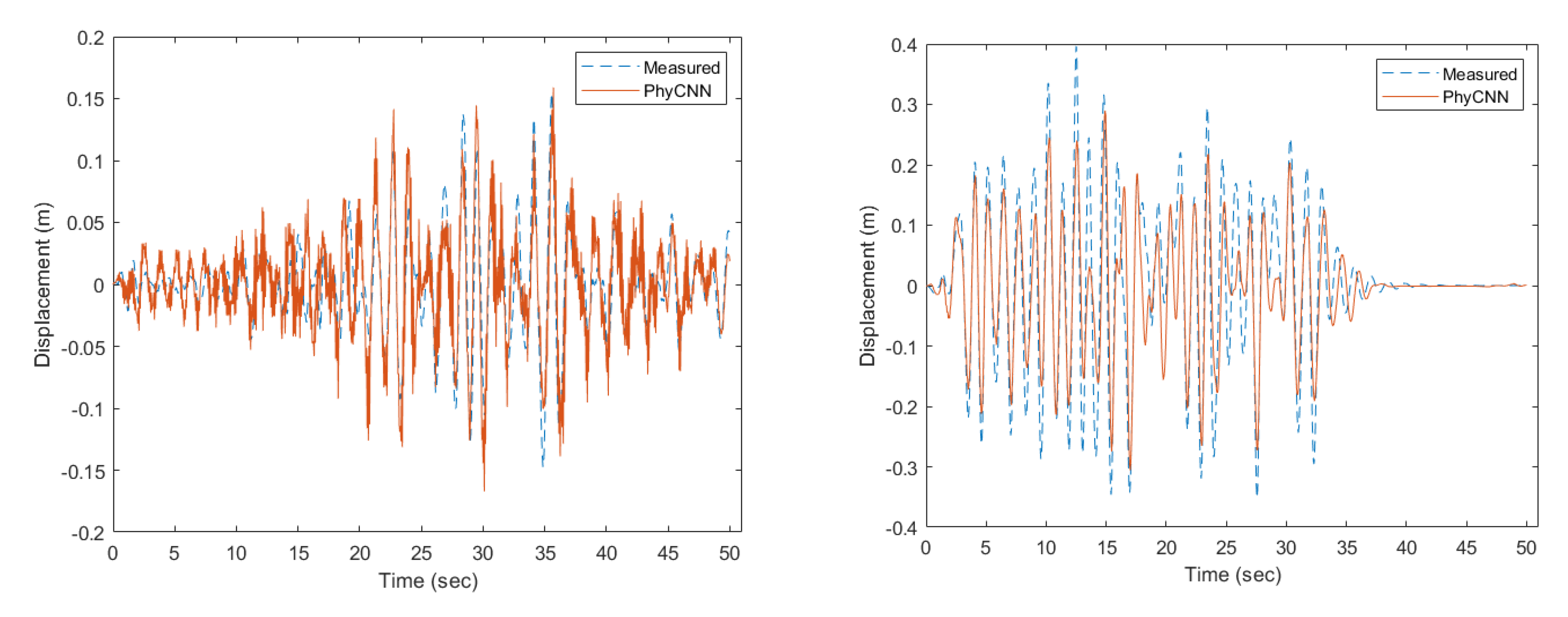
Figure 7 presents the prediction results of the PhyCNN model by Zhuang and colleagues [
17] for the same SDOF structural system as in
Figure 6. It provides a comparative basis for evaluating the performance of the FuzzyCNN model. The PhyCNN model is another neural network-based approach that focuses on leveraging physical principles in the prediction process. The comparison between FuzzyCNN and PhyCNN predictions is essential to understand the advantages and limitations of each model. While the PhyCNN might excel in scenarios where physical laws are well-defined and can be directly incorporated, it may struggle with uncertainties or data-driven nuances that the FuzzyCNN can address through its fuzzy logic components.
To facilitate a more robust comparison of the results between two models, the correlation coefficient has been employed. The correlation coefficient is a statistical measure used to assess the strength and direction of a linear relationship between two variables.
where
represents the number of data points,
is the recorded values,
is the computed values, and
is the mean of the recorded values. In this context, it measures the correlation between predicted and actual values for the structural system’s response.
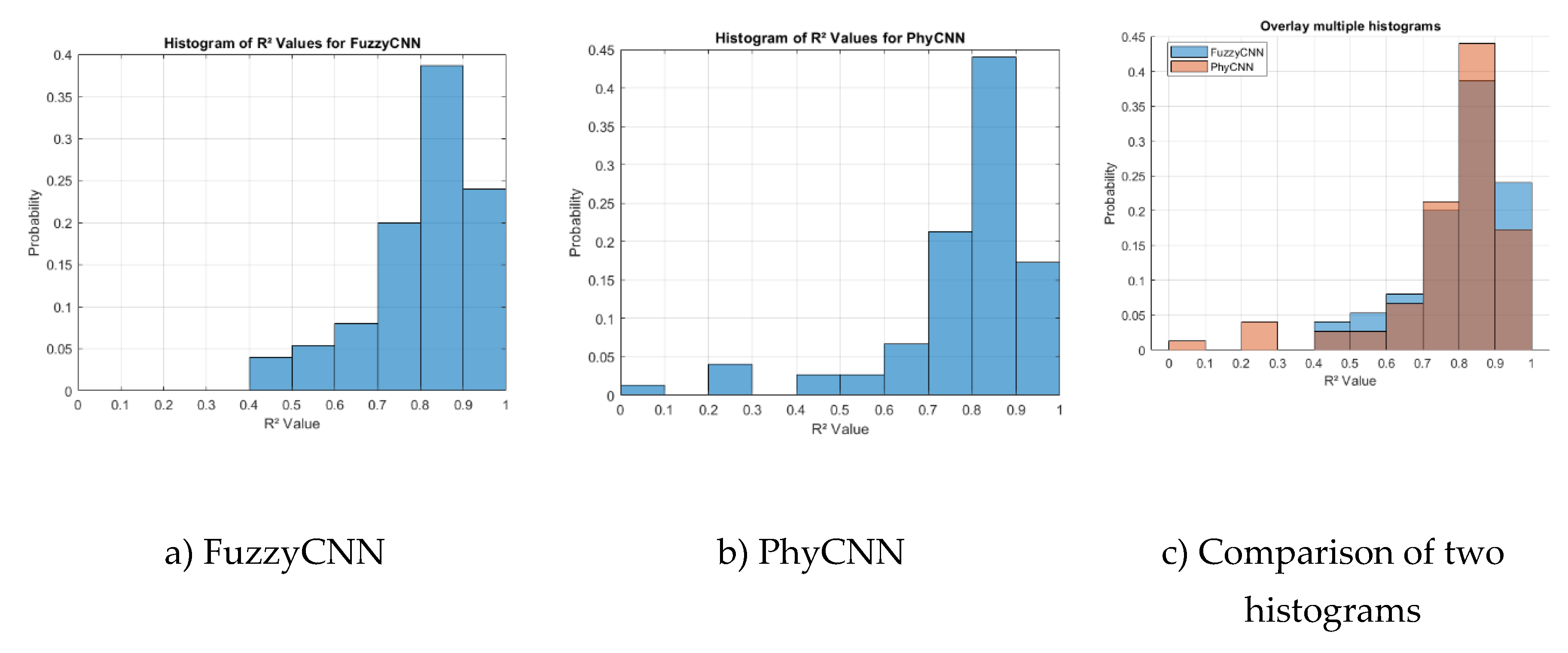
The histograms (
Figure 8) provide a visual representation of the distribution of correlation coefficients obtained from various predictions made by the models. The histogram for the FuzzyCNN model (
Figure 8a) shows how well this model’s predictions correlate with actual data. A peak towards higher correlation values indicates better model accuracy. The PhyCNN model’s histogram (
Figure 8b) serves a similar purpose.
Figure 8c allows for a direct comparison between the two models, highlighting any differences in performance. For instance, a broader distribution in one histogram might suggest that a model performs inconsistently across different scenarios (like PhyCNN), while a tighter distribution with higher correlation values would indicate consistent and accurate predictions (like FuzzyCNN). It appears that nearly 5% of the predictions made by the PhyCNN model have an R² value lower than 0.4. An R² value of 0.4 or lower signifies that the model explains less than 40% of the variance in the dependent variable based on the independent variables. In practical terms, this means that the model’s predictions are not closely aligned with the actual outcomes for those specific cases. Such a low R² indicates a weak predictive power, suggesting that the model’s performance is inconsistent across the dataset. The PhyCNN model’s dependence on directly integrating physical concepts into the neural network can be advantageous and disadvantageous at the same time [
37]. This method guarantees that forecasts follow established physical rules, but if the physics is not precise or complete for all possible circumstances, it might not fully represent the complexity of the data. The PhyCNN model’s overall dependability and credibility may be impacted if a subgroup of predictions has such low R
2 values. Even a tiny fraction of inaccurate forecasts can have a big impact on crucial applications like safety evaluations or structural engineering, sometimes resulting in dangerous choices or wrong conclusions [
38].
Based on
Figure 8, it appears that for the PhyCNN model, almost 17 percent of predictions have an R² higher than 0.9, while for the FuzzyCNN model, almost 24 percent of predictions have an R² higher than 0.9. The higher percentage of predictions with R² values above 0.9 in the FuzzyCNN model suggests it has a more flexible architecture, capable of adapting to a wider variety of data patterns. This flexibility may be attributed to the integration of fuzzy logic, which helps manage uncertainties and non-linearities in the data. One reason for the poorer performance of PhyCNN could be its sensitivity to noise present in earthquake records [
38]. Noise in earthquake recordings can significantly impact the performance and reliability of PhyCNN models. These models are designed to leverage physical principles, making them sensitive to data quality. Earthquake data, however, is often contaminated with various types of noise, including ambient environmental noise, instrument noise, and interference from human activities or other seismic events [
38]. This noise can obscure critical features within the seismic waveforms, such as amplitude, frequency content, and phase, which are essential for accurate modeling and interpretation [
38]. Consequently, when the PhyCNN model encounters noisy data, it may struggle to extract meaningful patterns, leading to reduced accuracy in its predictions [
38].
Additionally, the PhyCNN model contains approximately 207,414 more parameters than the FuzzyCNN model. This significantly larger parameter count suggests that PhyCNN may have a higher capacity for learning complex patterns, but it also carries a potentially increased risk of overfitting, particularly when dealing with limited datasets. The trade-off between model complexity and generalization ability should be carefully considered in the context of the available training data and the specific task at hand [
36]. In other words, the PhyCNN may unintentionally learn to identify noise patterns as meaningful features if the training set contains noisy recordings. This overfitting weakens the model’s robustness in real-world applications, where noise characteristics can differ greatly, as well as its capacity to generalize to new, unseen data [
39].
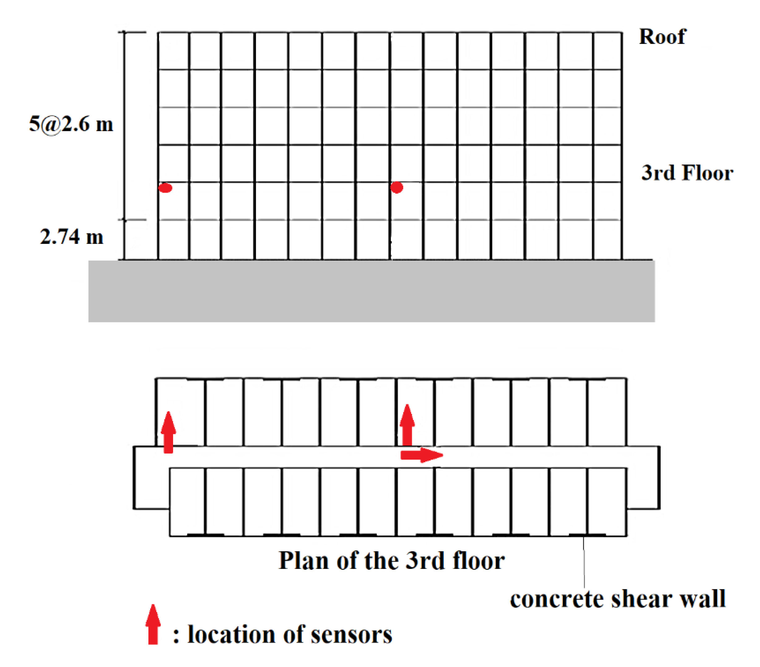
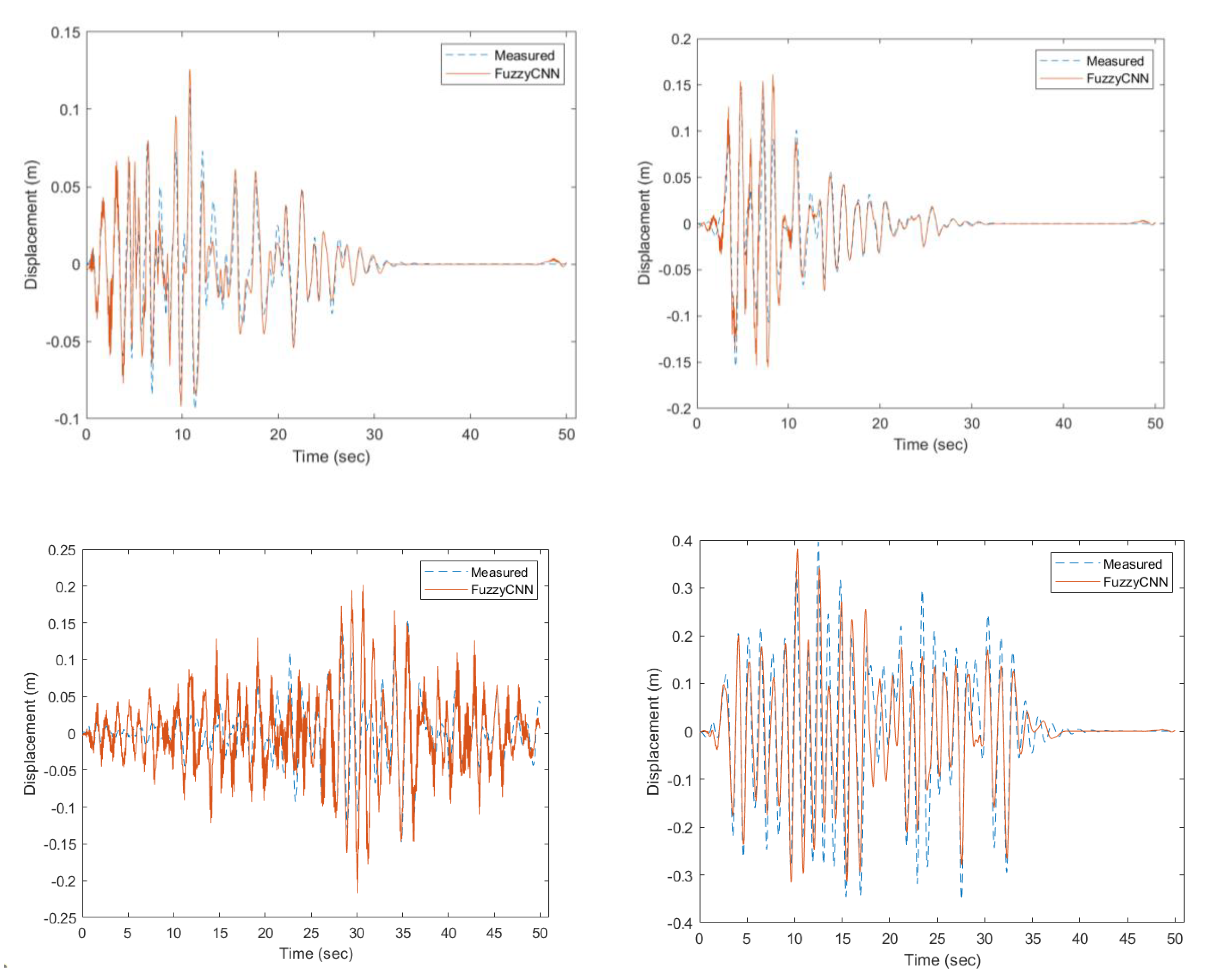
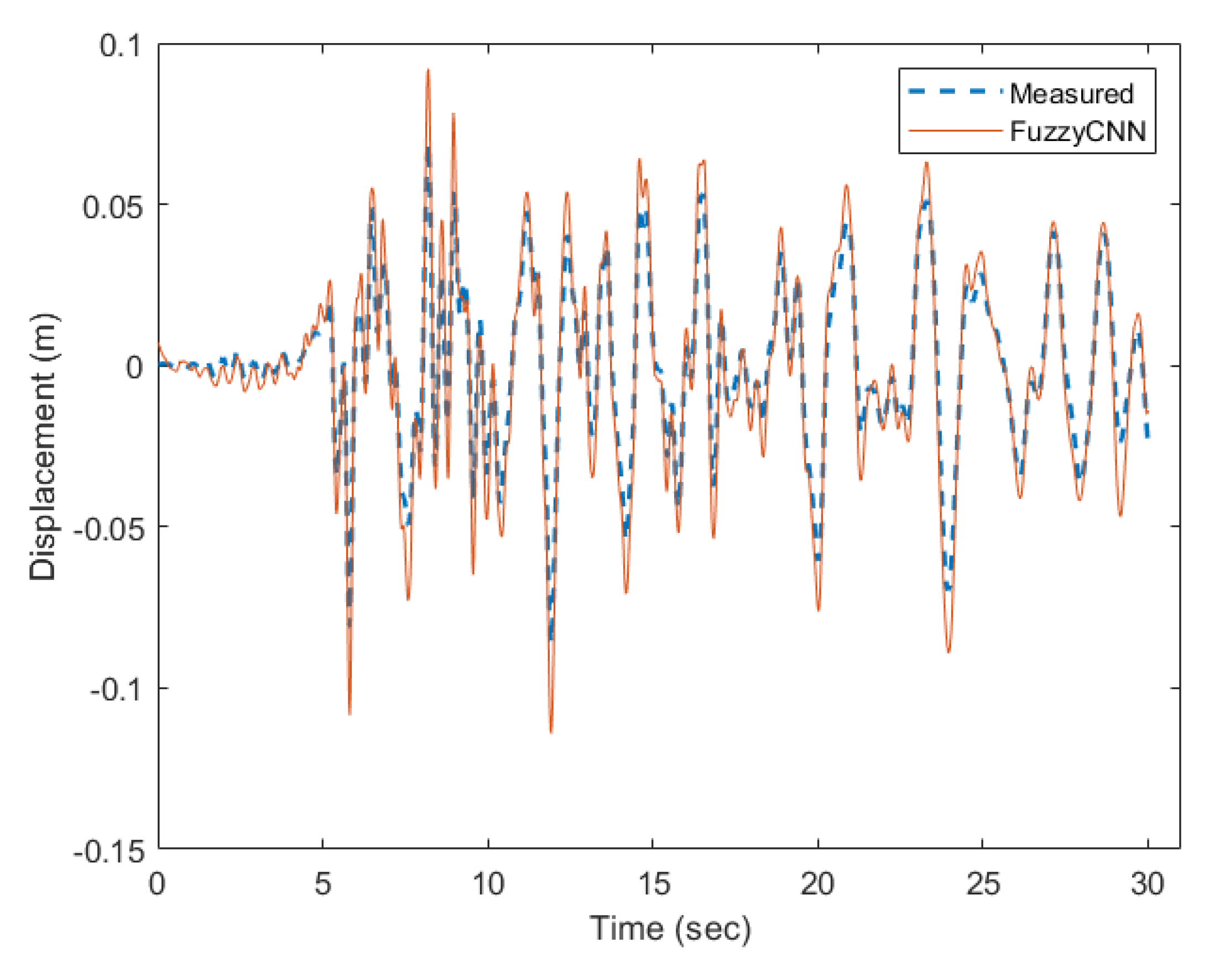
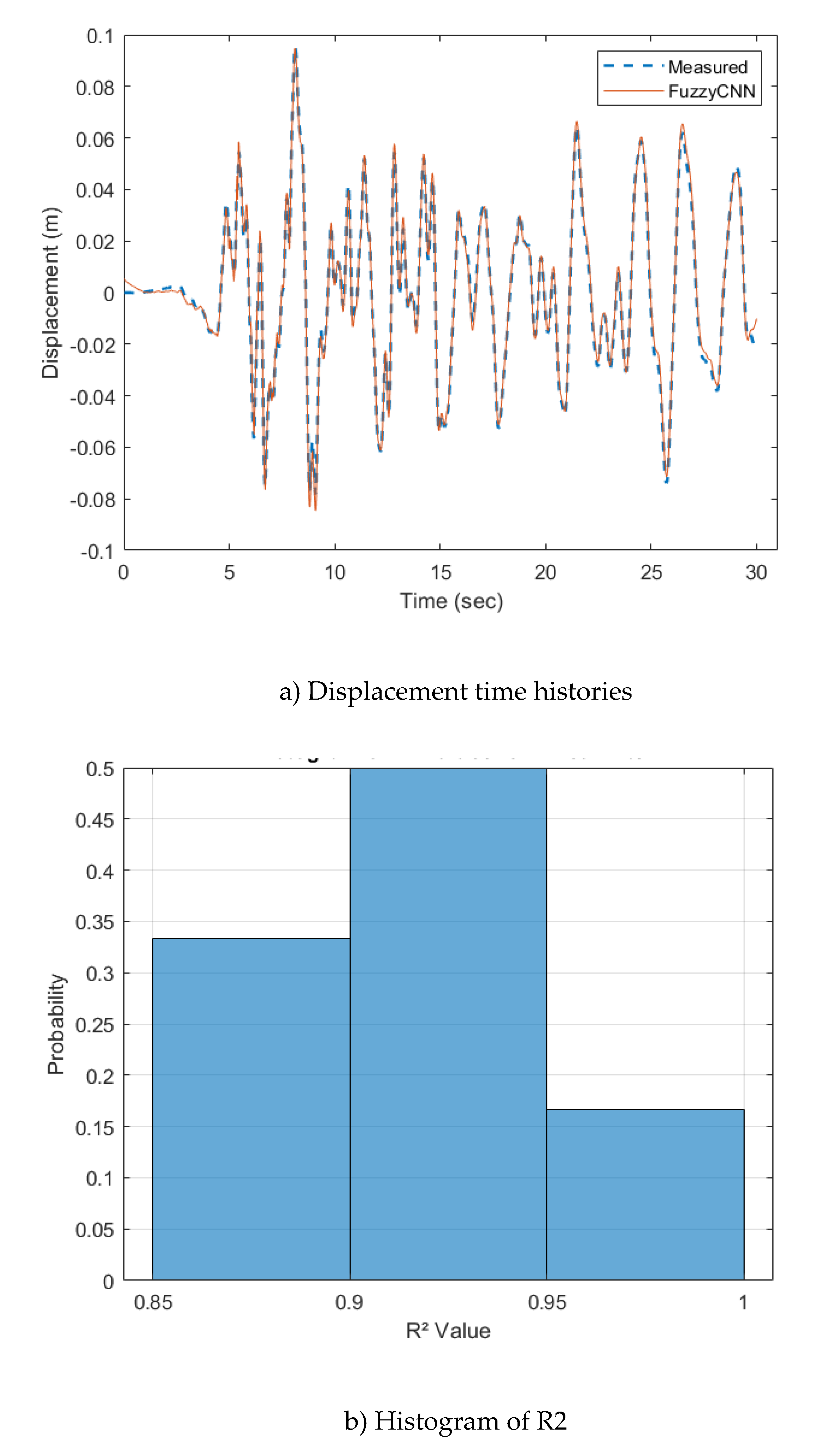
Figure 9 shows the performance of FuzzyCNN for the prediction of the displacement of the six-story mid-rise hotel building.
Figure 9a displays examples of the estimated displacement time histories on the 3rd floor. The predictions made by the FuzzyCNN show good agreement with the reference data in terms of residual displacement suggestive of plastic deformation, phase alignment, and amplitude. These characteristics of the model’s capturing accuracy indicate that it is a good emulation of the underlying physical phenomena and structural reactions. Moreover, as
Figure 9b illustrates, the correlation coefficients primarily surpass 0.85, highlighting the strong prediction model precision. This high degree of accuracy shows that the FuzzyCNN is a reliable tool for sophisticated structural analysis and simulations because it can accurately predict the complicated, nonlinear behaviors that are inherent in materials undergoing plastic deformation. The model’s resilience and dependability in real-world applications are highlighted by the consistency in both magnitude and phase as well as the rarely observed differences in residual drifts.
5. Conclusions
This study addresses the critical challenge of accurately predicting the dynamic response of nonlinear structural systems to seismic events. Traditional methods often struggle with computational intensity and the ability to generalize from limited datasets, necessitating the development of more efficient and robust approaches. The research introduced the Fuzzy Convolutional Neural Network (FuzzyCNN) model, which integrates fuzzy logic with convolutional neural networks to enhance the prediction accuracy of structural responses under seismic loading. Compared to the PhyCNN model, FuzzyCNN demonstrated superior performance, achieving higher correlation coefficients and greater robustness to noise in seismic data. Specifically, 24% of FuzzyCNN predictions had coefficient of determination (R²) values above 0.9, indicating a strong predictive capability, while only 17% of PhyCNN predictions reached the same threshold.
Additionally, about 5% of the predictions from the PhyCNN model had R² values lower than 0.4, highlighting its comparative underperformance in certain scenarios. The FuzzyCNN model’s integration of fuzzy logic enables it to manage uncertainties and nonlinearities more effectively than traditional physics-informed neural networks. This adaptability allows FuzzyCNN to provide more consistent and accurate predictions across diverse seismic events, highlighting its potential as a valuable tool in structural engineering. The study’s findings suggest that incorporating fuzzy logic principles into neural network architectures can significantly enhance their performance in modeling complex dynamic systems. Also, the field measurements of the six-story concrete structure in San Bernardino used in this research indicate that the predictions align closely with historical sensing data for earthquakes of varying magnitudes and frequency. This suggests a strong correlation between the modeled predictions and actual seismic activity observed in the area, demonstrating the effectiveness of the predictive models employed in the study.
In conclusion, the FuzzyCNN model represents a significant advancement in predicting structural responses under seismic loading. By effectively combining fuzzy logic with convolutional neural networks, it offers a robust and adaptable solution for structural engineers. Ongoing refinements aim to ensure its practical application in mitigating seismic risks, highlighting the potential of advanced machine learning techniques integrated with traditional engineering principles for the future of structural dynamics.

