1. Introduction
The functionality and longevity of components in technical systems are significantly influenced by their lubricated tribological contacts, such as those found in seals. Understanding the tribological interactions is challenging due to the complex phenomena involved. Dynamic friction, primarily governed by fluid dynamics, is crucial for accurately describing these interactions. Analytical models often require simplifications that exclude some phenomena, leading to inaccuracies. Experimental methods for understanding tribological behavior are typically costly and time-intensive. A commonly used approach is modeling the system with elastohydrodynamic lubrication (EHL) simulations, which employ the Reynolds equation to compute pressure distribution and contact surface deformation. [
1]
At the Institute for Fluid Power Drives and Systems (ifas) of RWTH Aachen University, an EHL simulation model for reciprocating seals, known as ifas-DDS (Dynamic Description of Sealings), was developed [
2,
3,
4,
5]. This model calculates friction by solving the hydrodynamic equations within the sealing contact using the Reynolds equation while also accounting for contact mechanics and seal deformation [
6]. Previous studies have validated this EHL model against experimental data [
7]. This approach’s significant drawback is the computational time required to solve the equations numerically. While increasing computational resources could alleviate this issue, it is often not practical, significantly as the complexity of simulations increases, and real-time computation is needed for applications like control systems.
Machine learning algorithms, such as neural networks (NNs), offer a promising substitution for traditional EHL simulations due to their rapid computation capabilities following initial training. The primary goal of using an NN, usually in regression tasks, is to minimize the deviation between the network’s predictions and the desired outcomes. This purely data-driven approach might yield good predictions for the training data. Still, it may result in overfitting, causing high errors for new data points within and especially outside the training domain due to a lack of physical understanding. An advancement in the field of NNs is the development of physics-informed neural networks (PINNs), which address this issue by incorporating physical laws into the network’s training process, thereby improving predictive accuracy across unfamiliar data. PINNs are a class of machine learning solvers for partial differential equations (PDEs). Unlike traditional NNs, their training process is not solely data-driven. The optimal parameters of a given network structure are determined by a loss function, which, in the case of PINNs, includes physical laws described by the residuals of the PDEs and the initial and boundary conditions.
Several studies have concentrated on the hydrodynamic aspect of EHL simulations, excluding deformation and friction. Recent developments, such as the studies by Almqvist [
1,
8,
9,
10,
11], highlight the potential of PINNs to combine the precision of distributed simulation models with the computational efficiency of NNs, ensuring robust, accurate, and faster computations. However, these studies have primarily modeled hydrodynamics involving either stationary cavitation or geometry changes without cavitation. There remains a gap in research on applying PINNs to transient cavitation scenarios, both with and without geometry changes.
This study explores the capability of PINNs in addressing the Reynolds equation under conditions of sliding and squeezing motions, as well as in modeling transient cavitation within sealing contacts, building on a previously successful application of the hydrodynamic-PINN (HD-PINN) framework for stationary cases without cavitation [
9], this research extends the framework to two specific scenarios: a curved sealing geometry with a flat counter surface with a dynamic change in the gap height and a fixed sealing geometry. Furthermore, the framework is extended by two features, which are soft constraints and collocation point updates, to enhance the accuracy of the PINN. Consistent with earlier studies, the focus here is on the hydrodynamic aspects of elastohydrodynamic lubrication (EHL), with pressure and cavitation distributions being calculated while omitting considerations of friction and contact mechanics [
1]. Deformation is artificially modeled by a constant seal movement, ignoring any pressure dependencies.
The subsequent section outlines the model used for hydrodynamic lubrication.
Section 4 offers a general overview of PINNs, while
Section 5 delves into the HD-PINN framework, the implemented modifications, the specific scenarios analyzed, and the physical loss terms. The results, discussed in
Section 6, are validated using a modified variant of the ifas-DDS, known as the rigid DDS, which excludes the earlier mentioned EHL factors. The final section,
Section 7, summarizes the results and provides a conclusion.
3. Hydrodynamic Lubrication Reynolds Equation with transient Cavitation Modeling
Friction and wear are significant factors in tribological systems. They can be analyzed with EHL simulations, which examine the dynamic interactions within lubricated contacts by modeling surface deformations and calculating hydrodynamic pressure within the gap. The results of these simulations are often utilized to design and optimize tribological contacts such as those found in dynamic seals or, more specifically, in valves. [
1]
The ifas-DDS is a sophisticated simulation tool designed to solve the hydrodynamic interactions between a seal and its counter surface in small gaps. Using the Reynolds equation, a finite solver computes the pressure distribution within the lubricating film. Abaqus, a finite element software, is utilized to simulate the deformation of the seal. Dependencies between pressure and deformation are seamlessly integrated into Abaqus through custom user subroutines. Previous studies have validated these simulation results against experimental data. [
7]
This study describes hydrodynamics as defined by the Reynolds equation, excluding contact mechanics, pressure-dependent surface deformation, and friction. The primary objective is to investigate lubricated contacts and assess how the PINN handles the constant movement of the seal, which will be modeled as pressure-dependent deformation in the next phase of the study. Furthermore, the study examines the potential of PINNs to model transient cavitation, which has not been explored in existing research, where cavitation studies, such as Rom’s work [
10], have focused on stationary cases.
The prediction of the PINN framework is compared to the rigid DDS. This model does not incorporate the Abaqus integration and thus neglects deformation, friction, and contact mechanics, focusing exclusively on lubrication dynamics. Both PINN and rigid DDS solve the same underlying equations, allowing for direct validation of the PINN’s predicted outputs. Cavitation in the fluid film is modeled according to the Jakobsson-Floberg-Olsson cavitation model. This model assumes the gaseous phase formation due to vaporization or the air dissolution in the fluid if the local pressure drops below a certain threshold (in this study
). Cavitation is characterized by the cavity fraction
[
6], which represents the local gaseous volume fraction, ranging from 0 (no cavitation) to 1 (full cavitation).
The investigated Reynolds equation is an extension of the original version by integrating the cavity fraction
as follows [
6]:
The Reynolds equation is used to describe the hydrodynamic pressure
p within a small lubricated gap. The pressure, as a function of position
x and time
t, depends on numerous additional parameters: the relative velocity
v between the contact surfaces, the fluid’s density
the gap height
h, the viscosity
, and the derivatives of pressure with respect to time and position,
and
. The pressure flow factor
and the shear flow factor
represent the surface roughness according to the averaged flow model by Patir and Cheng [
12,
13]. Further parameters are the root mean square roughness of the contact surfaces
and the density
, which is neglected since the fluid is assumed to be incompressible, changes in
are considered to be zero, allowing the Reynolds equation (Equation
1) to be simplified by dividing by
.
The cavity fraction
denotes the extent of cavitation within the lubricated contact and occurs when the pressure drops below the vaporization threshold. The vaporization threshold is set to zero in this research. To obtain a relationship between pressure and cavity fraction, according to the implementation by Woloszynski et al. [
14] the Fischer-Burmeister Equation is used:
Since the JFO cavitation model and its implementation make little assumptions about the physical mechanisms causing the cavity fraction
to become non-zero, the model can also be used for tracking the distribution of the lubricant in tribological contacts with only a limited amount of lubricant supply (starved lubrication), e.g., grease lubricated sealing contacts in pneumatic spool valves. In this case, a non-zero value of the cavity fraction does not necessarily denote the occurrence of cavitation but rather a partial filling of the sealing gap at the corresponding location. For a better interpretation of the partial filling, the lubricant film height
is introduced. The lubricant film height is defined as the local film height and computed as follows:
Further details about the implementation of this model for describing contacts with starved lubrication in the EHL model will be published in a subsequent paper.
4. Physics-Informed Neural Network
The pressure distribution in narrow lubricated contacts is characterized by the Reynolds equation (eq.
1) described in the prior section. In its complete form, no analytical solution of this equation exists. It necessitates using computationally demanding numerical methods such as finite element or finite volume methods to simulate hydrodynamic and tribological issues.
In the field of tribology, machine learning has gained popularity in the last few years due to substantial progress [
15,
16]. In fault detection, NNs have been successfully applied in systems like slipper bearings, journal bearings, and ball bearings [
17,
18,
19]. Regarding EHL simulations, Hess et al. determined the elastohydrodynamic pressure distribution with a convolutional neural network within journal bearings [
20]. Two main reasons for the advancements of machine learning algorithms applied to tribological interfaces are the vast availability of open-source machine learning libraries, e.g., PyTorch and TensorFlow, and the algorithms’ adaptability. However, one drawback of these data-driven models is their black-box characteristics and lack of transparency. Hybrid models that combine physical rules with data-driven methods have been developed to address this issue. These models benefit from reduced data requirements and an implementation based on physics described by mathematical equations [
21]. The structure of these hybrid models can be implemented in a sequential, a parallel, and a structured configuration [
22,
23,
24].
Integrating data and mathematical physics models in machine learning algorithms, known as physics-informed machine learning (PIML), enhances traditional models by increasing their accuracy and robustness for applications in lubrication, friction, and wear prediction [
25]. Embedding physical rules into NNs, alongside the classical data-driven approach, results in implementing hybrid PINNs. These often provide more robust and precise solutions compared to purely data-driven networks. Physical laws are incorporated through residual terms that describe the underlying equations of the investigated systems. These terms are included in the loss function by solving them with the output of the PINN and, if applicable, the derivatives of the output [
26].
Following the work of Hornik and Cybenko, who derived that deep NNs can approximate any continuous function to a certain level of accuracy [
27,
28], Hyuk extended this theory to include Borel measurable functions [
29]. The early contributions to physics-based regularization in NNs were made by [
29,
30]. Although Lagaris and Hyuk did not explicitly utilize the term "physics-informed," their research closely reflects the core concepts of what is now recognized as PINNs. Hyuk’s key innovation was to modify the NN’s loss function to integrate the governing differential equation, laying the groundwork for developing PINNs. This concept of embedding physical laws into NN training has significantly influenced the evolution of PIML, which combines traditional machine learning with domain-specific knowledge. Due to the limited computational resources and the early state of computational algebra techniques, this approach did not gain widespread attention. Recent progress in gradient calculation methods (e.g. (AD)), and significant improvements in hardware processing power, opened up new potential.
A decade ago, Owhadi incorporated prior physical knowledge into the solving process of an NN, causing the resurgence of PIML. He formulated the solution of PDEs as Bayesian inference tasks, improving the algorithms with problem-dependent knowledge [
31]. Next, Raissi et al. developed a probabilistic machine learning algorithm to solve general linear equations via the Gaussian process, refining it for integro-differential or partial differential equations [
32,
33]. Furthermore, this algorithm was upgraded to compute nonlinear partial differential equations [
34,
35].
A significant advancement was the development of PINNs, which, compared to finite element solvers, can be described as mesh-free models that transform the solving process of PDEs into an optimization task dictated by loss function [
36]. Raissi utilized PINNs as a new class of hybrid solvers, capable of determining solutions to various forward and inverse problems described by PDEs with high accuracy [
37,
38,
39]. Antonello et al. continued the previous research and extended the PINN concept to control tasks by adding control inputs into the network, building an algorithm capable of solving control applications [
40].
Figure 1 demonstrates a PINN with two inputs and one output. With the gradients calculated by automatic differentiation (AD), a hybrid loss is computed using physics-informed and data-based information.
PINNs process inputs, such as parameters and variables like spatial coordinates x and time t, like traditional NNs: The input values are passed through multiple layers, each consisting of neurons that are interconnected with those in both the preceding and subsequent layers. Within each neuron, the input is multiplied by a weight, a bias term is added, and the resulting value is then passed through an activation function. This series of operations across the network layers culminates in generating complex, nonlinear functions representing the network’s output.
For PINNs, the residual loss corresponds to the residual of the underlying physical equation, aligning with the principles of unsupervised learning [
41]. The spatial and temporal evaluation points, where these residuals are calculated, are called collocation points. PINNs leverage AD to compute gradients of any order [
42] for complex differential equations with machine-level accuracy, utilizing the chain and product rules. Unlike traditional NNs, where AD is primarily used for parameter updates during training, PINNs also employ it to calculate the necessary derivatives of the physical equations.
In addition to the residual loss, PINNs can incorporate boundary condition (BC) and initial condition (IC) losses, which are implemented as supervised losses. As illustrated in
Figure 1, additional types of losses may arise depending on the specific problem setup. An example of this is the hybrid PINN approach, where existing data is integrated to accelerate and enhance the accuracy of the solution, resulting in a data loss term.
The following section provides a brief overview of the application of PINNs in the field of hydrodynamics.
The first publication utilizing PINNs in the field of hydrodynamics addressed the solution of a simplified Reynolds equation [
8]. Subsequent research by Yadav et al., Li et al., and Zhao et al. refined this approach, expanding the method to solve two-dimensional equations for tackling more complex problems [
43,
44,
45]. Notable progress was made by Rom, who successfully applied PINNs to solve the Reynolds equation incorporating the Jakobsson–Floberg–Olsson (JFO) cavitation model for stationary problems. Rom further enhanced the methodology by introducing soft constraints and adding collocation points during training, significantly improving the accuracy of the predicted cavitation distribution, particularly in regions with high gradient variations [
10].
Further progress in the application of PINNs to hydrodynamics was made by Cheng et al., who solved the Reynolds equation incorporating both the JFO and Swift-Stieber (SS) cavitation models [
46]. Building on this work, Xi et al. enhanced the solution by implementing a combination of hard and soft constraints [
47]. In the previous publication, we demonstrated that PINNs are capable of predicting solutions to the stationary Reynolds equation across a wide range of parameters [
9].
Rimon et al. utilized PINNs to model the deformation of rotary shaft seals, applying a simplified Reynolds equation in conjunction with the Lamé equation to account for material dependencies [
11]. This approach allowed for a more comprehensive description of the interactions between fluid dynamics and material deformation, highlighting the potential of PINNs in solving complex, coupled physical problems.
While these contributions have demonstrated considerable advances in addressing the Reynolds equation through the use of PINNs, it is crucial to recognize that most studies have primarily concentrated on the implementation of PINNs. However, a comprehensive hydrodynamic lubrication PINN framework extends beyond the PINN itself. Such a framework encompasses a broader set of components including the automated tuning of hyperparameters, strategic initialization of weights tailored to the specific activation functions employed, and sophisticated loss balancing. These elements are pivotal in the learning process and are often underemphasized in existing literature, where hyperparameter tuning and loss balancing frequently involve substantial manual experimentation.
4.1. Physics-Informed Neural Network for Solving the Reynolds Equation
The original study utilizing PINNs to address a simplified form of the Reynolds equation was conducted by [
8]. Subsequent investigations have further refined this approach by developing more sophisticated algorithms that tackle the 2D Reynolds equation in various applications such as gas bearings, linear sliders, and journal bearings, respectively [
43,
44,
45]. Rom made a notable contribution by being the first to apply PINNs to the stationary Reynolds equation, integrating the JFO cavitation model. Furthermore, Rom enhanced the model’s adaptability to variable geometrical setups by incorporating relative eccentricity into the PINN’s input parameters [
10].
Building on these developments, Cheng et al. developed a PINN that can solve the Reynolds equation using either the JFO or SS cavitation models [
46]. Xi et al. have investigated the stationary Reynolds equation with cavitation, integrating both soft and hard constraints in their loss to improve the accuracy of their solutions [
47]. Brumand-Poor et al. successfully applied their HD-Framework to solve stationary cavitation and dynamic height changes of a sealing gap [
48]. Moreover, Rimon et al. have assessed the potential of PINNs for complete EHL simulations, solving a simplified variant of the Reynolds equation and modeling the deformation of seals via the Lamé equation [
11]. The previously mentioned research focused on smooth surfaces, in most recent times Brumand-Poor et al. investigated the Reynolds equation with rough surfaces [
49].
Table 1.
Overview of different NNs used in the literature for solving the Reynolds equation. Nomenclature: eccentricity , angle of attack , velocity in and leakage rate Q.
Table 1.
Overview of different NNs used in the literature for solving the Reynolds equation. Nomenclature: eccentricity , angle of attack , velocity in and leakage rate Q.
| Author |
Inputs |
Layers |
Layer Size |
Output |
| Almqvist [8] |
x |
1 |
10 |
p |
| Cheng et al. [46] |
x, y
|
6 |
20 |
p |
| Hess et al. [20] |
|
6 |
three-dim, see paper |
p |
| Ramos et al. [50] |
|
7 |
(4, 12, 50, 50, 25, 12, 1) |
p |
| |
|
6 |
(6, 15, 60, 60, 15, 1) |
p |
| Rimon et al. [11] |
x |
4 |
30 |
|
| Rom [10] |
|
6 |
20 |
|
| |
|
6 |
20 |
|
| Xi et al. [47] |
x |
3 |
64 |
|
| Zhao et al. [45] |
|
and 4 |
|
p |
5. HD-PINN Framework
This section will provide an overview of the later simulated test cases and then present the NN’s structure and functions.
5.1. Test Cases: Physics-Informed Loss and Conditions
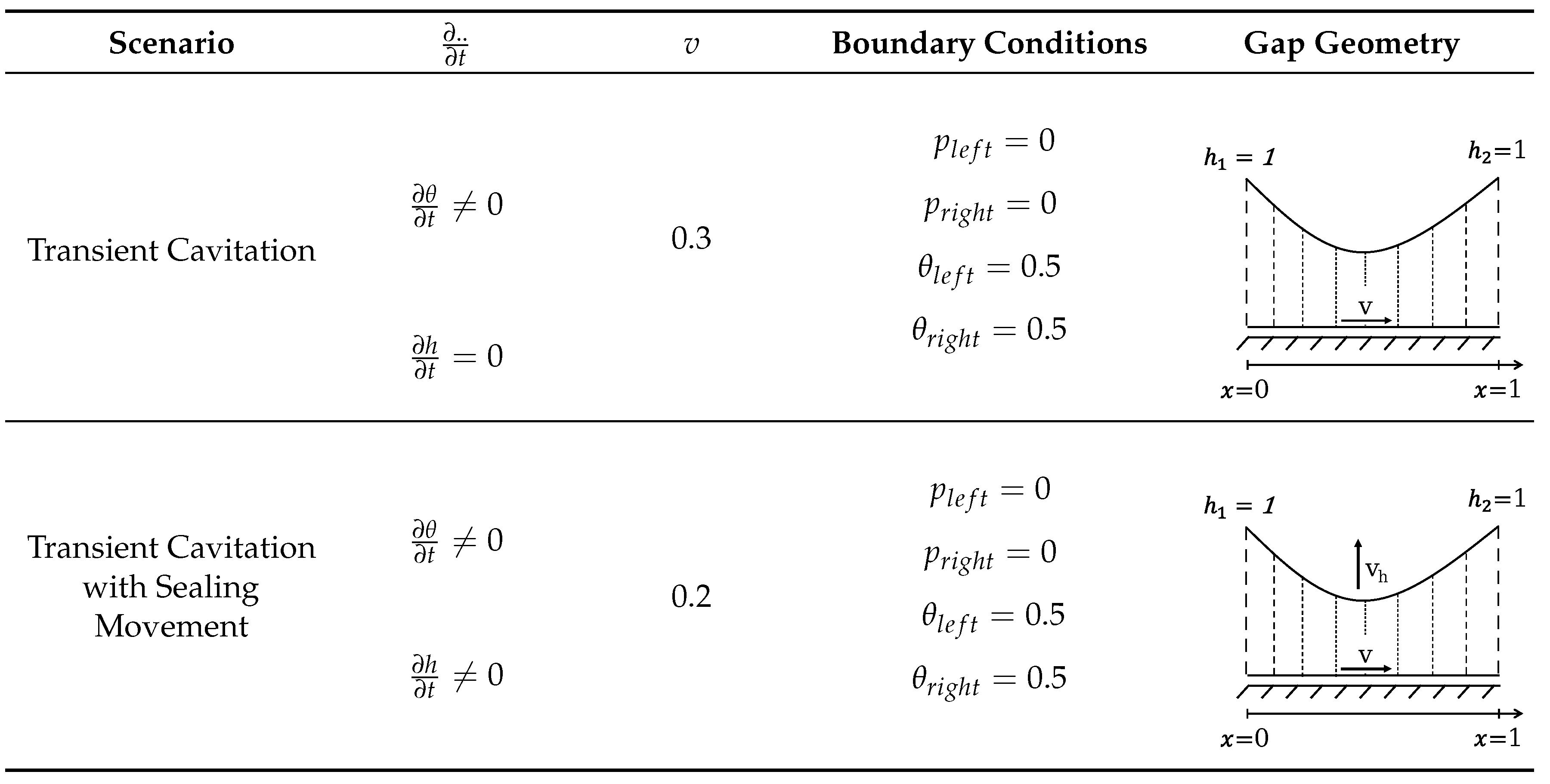
For this study, two different test cases are analyzed. The system consists of a curved rigid sealing geometry and a flat counter surface for both test cases. At
the film height is
at all positions where the gap height is higher than
. For all positions with smaller gap heights, film height and gap height are equal (i.e.,
). The boundary condition is 0 for the pressure and
for the cavity fraction at both boundaries. For the first test case, the seal (upper part of the gap) is kept stationary, with only the counter surface (lower part) moving horizontally. For the second test case, the seal is additionally moved vertically from the counter surface to model an inverse squeezing motion.
Table 2 gives an overview of the test cases.
To make an evaluation with the DDS possible, a test case with insufficient lubrication, meaning that the seal is only partly lubricated, is chosen. Hydrodynamic and surface parameters like
and
are set to one since they get normalized internally. Shear and pressure flow factors are neglected with
and
.
Table 3 and
Table 4 show all other simulation parameters.
5.2. PINN Structure
The network consists of 7 layers with 20 neurons, each with 17 inputs, including
x and
t and the different parameters and variables of the Reynolds equation. It outputs predictions for pressure
p and cavitation
.
Figure 2 provides a schematic illustration of the implemented PINN structure with the investigated loss terms.
The geometry describing the height profile between the sealing and counter surface is characterized by four coefficients over the position interval
as follows [
1]:
Five different losses, shown in
Figure 3 are used during training: The residual loss computes the extended Reynolds equation, needing an initial condition on the whole domain and boundary conditions for pressure and cavitation. Boundary and initial conditions are implemented as second and third losses. The Fischer-Burmeister equation is the fourth loss to model the relation between
p and
. Its loss alone has shown to be insufficient to predict transition areas where the cavitation approaches zero while the pressure approaches non-zero values or vice versa precisely. Therefore, a soft constraints loss is implemented, first used by Rom (see
Section 5.4).
Since different losses can vary in magnitude, they must be prioritized. A loss balancing is implemented inspired by previous work by Bischof and Kraus [
51]. This loss balancing algorithm, shown in
Figure 4 weights the five losses and adds them up to build the final loss for optimizing the NN.
5.3. Training Procedure
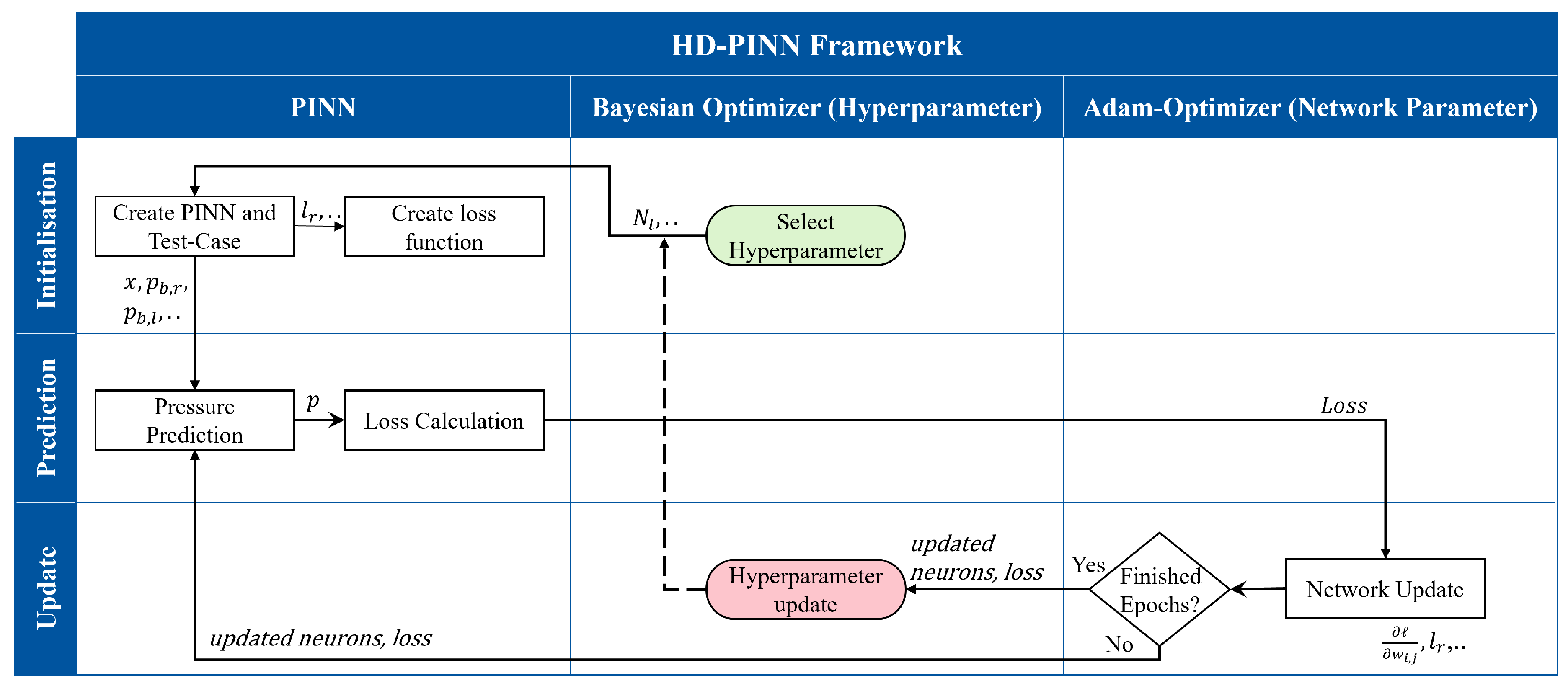
Bayesian optimization is used to find adequate hyperparameters (hp). This probabilistic finding of coherence between multiple unknown parameters returns a starting point for further optimization. An overview is shown in
Figure 5. Multiple training trials run in an outer loop until promising hps are found. For each training, a PINN and the corresponding loss functions are initialized. In the inner loop, predictions of
p and
are evaluated with the current neurons’ weights and biases for a predefined number of epochs. Consequently, the five losses are calculated. Adam optimizer then updates all neurons. Once all epochs are finished, a new trial is started. After finding promising hps, these can be further finetuned manually or a longer training session can be started to train a final NN.
Training runs are executed on a stand-alone computer with the following specifications: Intel I9 13th-generation processor, 128 GB RAM DDR5, and Nvidia RXT 4090.
5.4. Methods of Refinement
As mentioned in
Section 5.2, transition areas of cavitated to non-cavitated locations (or vice versa) need special treatment to predict pressure distributions accurately. Losses that are returned by the Fischer-Burmeister equation alone are usually not high enough to optimize the NN appropriately due to the small magnitude of
p and
in these areas. The soft constraints loss, first introduced by Rom [
10], solves this issue by putting extra emphasis on areas below a predefined threshold: Once either
or
are exceeded, the corresponding other value must be zero (see Equation
2) and therefore the predicted non-zero value is returned as loss. Furthermore, the loss is only normed over previously mentioned transition areas ignoring sectors below the threshold.
With the soft constraints implemented, training trials have sometimes been shown to predict distributions of both
p and
being zero. Though this satisfies the constraints of the Fischer-Burmeister equation (Equation
2), it does not satisfy the Reynolds equation. Therefore, the NN’s residual loss is increased by a factor of four in areas where the sum of
p and
falls below a threshold
.
High gradients have also been shown to be hard to predict. This is especially true for . Therefore, new collocation points are added to the domain in case absolute values of the -gradient exceed a certain threshold. These updates are triggered after a primary training period, and the NN can predict qualitative distributions. The process can be repeated every n epoch.
6. Results
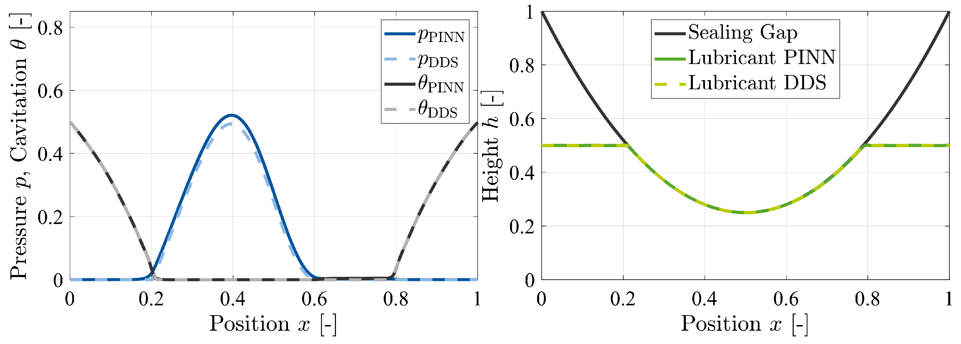
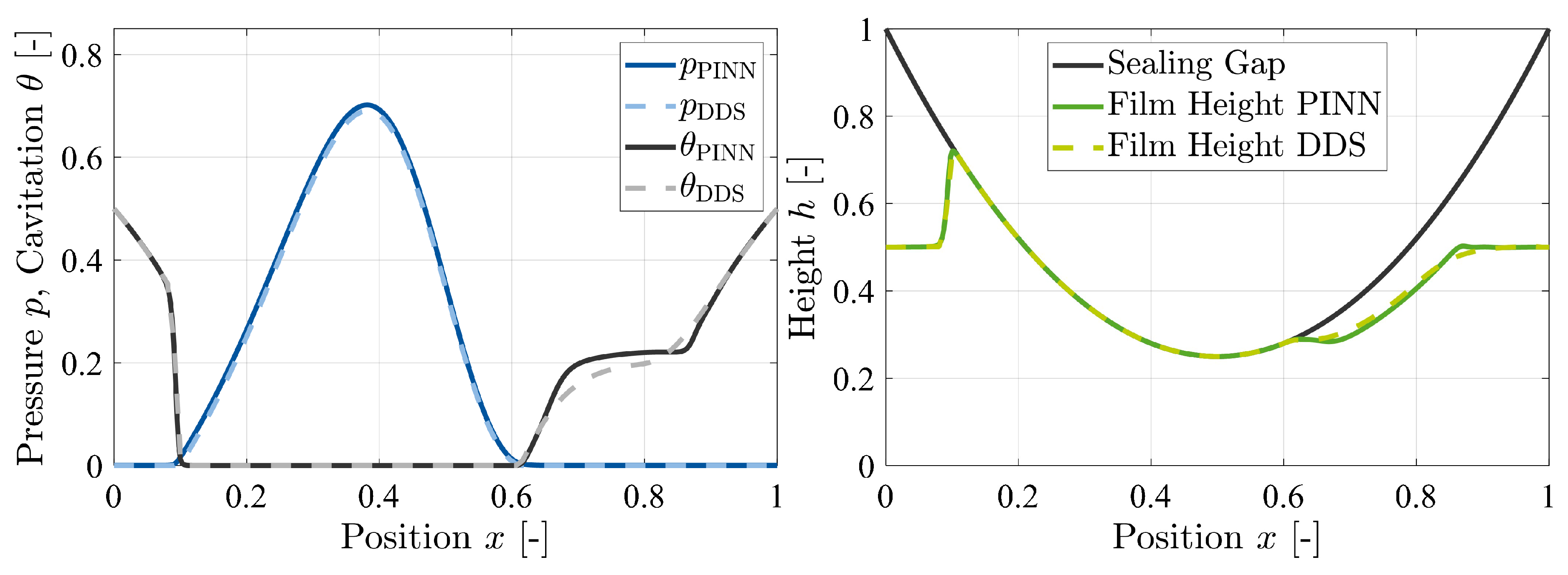
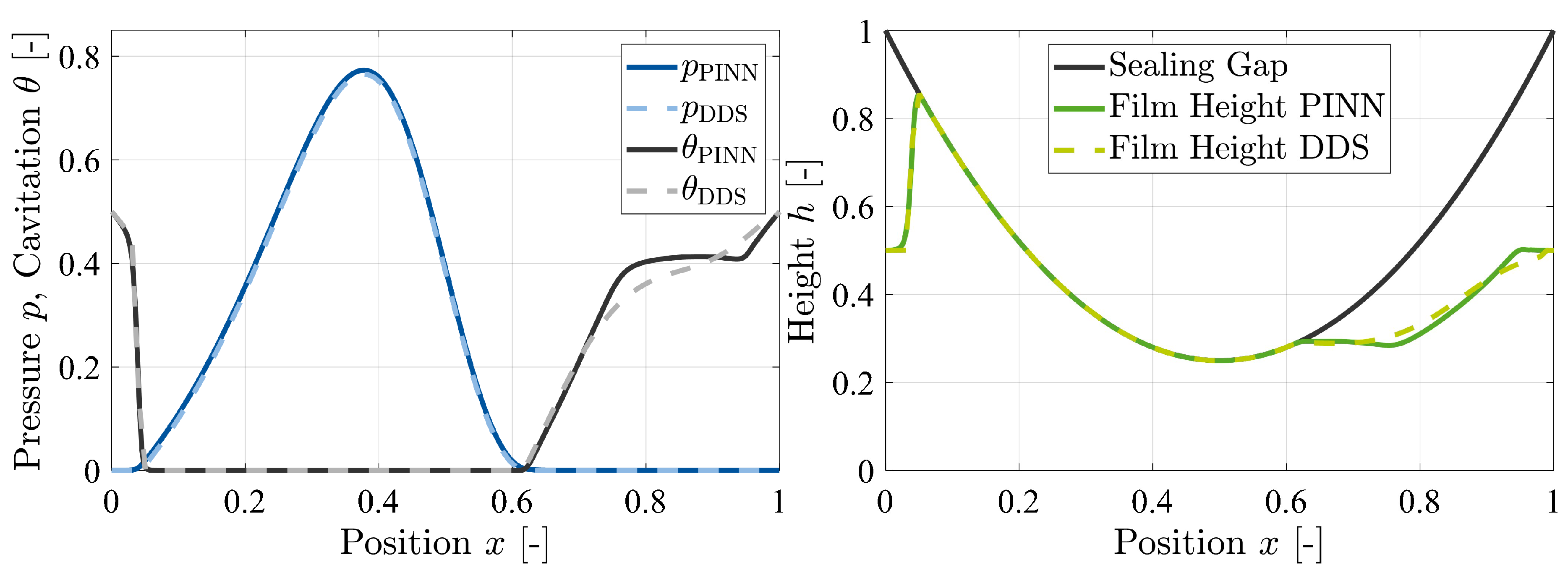
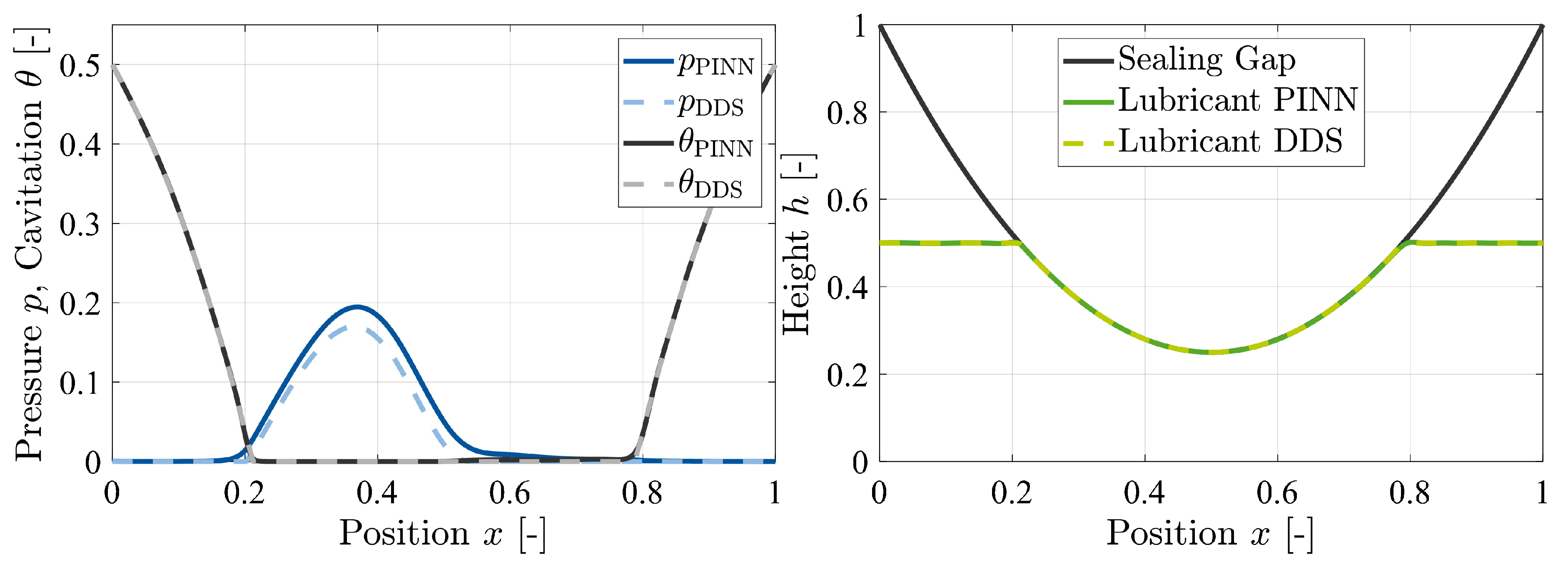
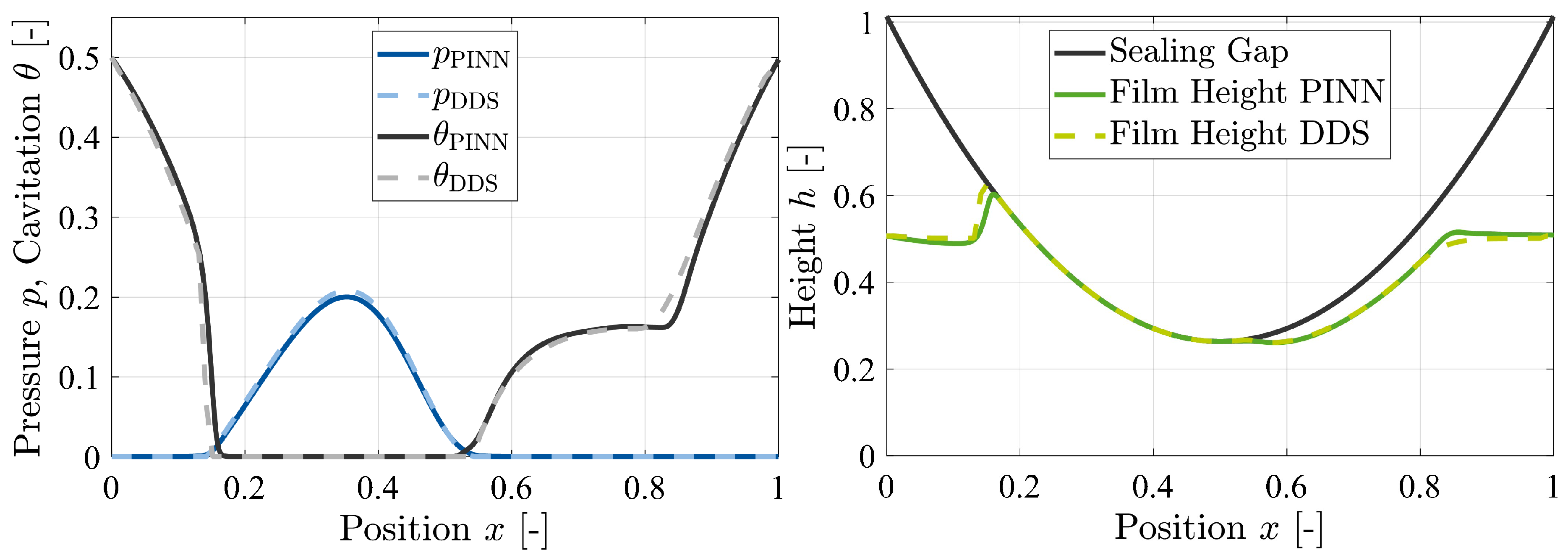
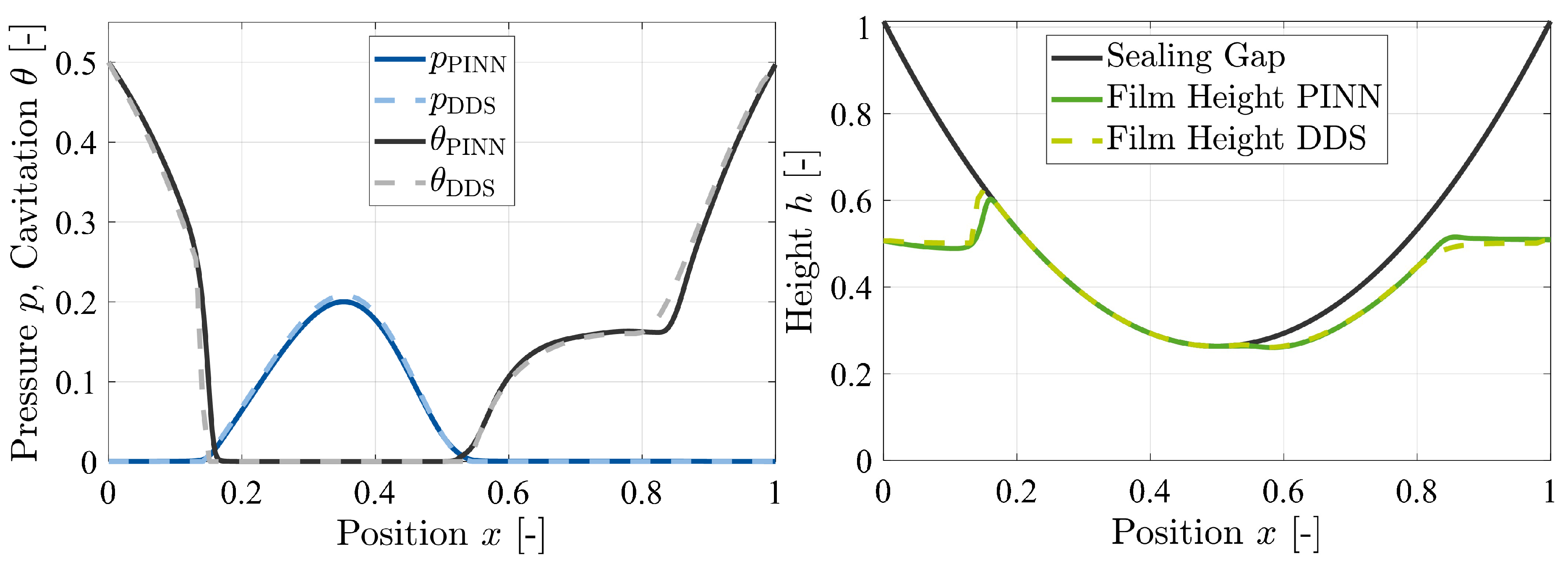
The following chapter presents predictions for the two test cases. As mentioned earlier, the cavity fraction is equal to at both domain boundaries for both cases and pressure, therefore, is supposed to be zero at these locations. Plots of predicted pressure and cavity fraction with the validation data from the DDS are shown for the three different time steps . For each time step, the position of the seal and the film height are plotted as well. Note that the film height is not an individually predicted output of the NN but rather the result of .
Ranges of the computed domain are and . The seal’s geometry is kept the same throughout this study.
6.1. Transient Cavitation
For the first case, the vertical velocity of the seal
is set to zero. All parameters can be seen in
Table 3. Predicted distributions are shown in
Figure 6,
Figure 7 and
Figure 8.
6.2. Transient Cavitation with Sealing Movement
The second test case models a vertical retracting movement of the seal. The housing still moves horizontally but
slower than in the first test case. Simulation parameters can be seen in
Table 4. The distributions are shown in
Figure 9,
Figure 10 and
Figure 11.
7. Discussion
7.1. Transient Cavitation
Computing a test case with transient cavitation, the PINN accurately predicts the general characteristics of the pressure and cavitation distribution. The magnitude and location of the pressure peaks are correctly evaluated, with averaged errors (over all time steps) for pressure and cavitation at and , respectively. Since changes in cavity fraction and film height do not occur instantly. Consequently, the two test cases are transient, meaning each time step depends on the previous one. Therefore, an initial condition is needed to compute a well-posed PDE. Note how the PINN handles this temporal dependence, with the pressure peak growing in magnitude and width.
Since the counter surface moves to the right, lubricant is impounded to the left of the seal. To its right, the film height decreases, creating a region of cavitation. The presented film height at a position x is the sum of all lubricated fractions at that position. It is assumed for modeling that at each position with , half of the lubricant sticks on the seal (top) and the other half on the counter surface (bottom). The plots do not contain any information on what part of the lubricant sticks on the bottom or top of the seal.
7.2. Tranisent Cavitation with Sealing Movement
The seal is slowly moved away from the counter surface in the second test case. All considered variables are non-zero. With suitable SC settings, an adequate general convergence can be achieved. The magnitude and location of the pressure peak are close to the simulated rigid DDS data in all time steps, with the averaged error being and for pressure and cavitation, respectively. A greater deviation can be observed in and , where the lubricant is impounded or transitions into a steady fluid film height, respectively. The sudden change in -gradient seems hard to fit. Especially in the last step, the cavity fraction diverts from the simulated ifas-DDS data (with an average error of ).
Soft constraint settings highly influence the position of pressure peaks. Since only first and second-order derivatives of the pressure are computed, the positions of the start and end of the pressurized area highly influence the peak’s overall magnitude. From experience gathered during multiple training trials, it can be said that values of
and
should be close together to ensure the pressurized area to be predicted at the right
x-position. Values that are too close together showed no plausible pressure distributions at all. Pressure values are zero for the whole domain (which also satisfies the Fischer-Burmeister equation (Equation
2)): A good trade-off was found to be
. Note that the ratio and, more importantly, the absolute values need to be tuned, as shown in the unreduced fraction.
Hydrodynamic predictions calculated by the PINN take about ms of execution time, while the iterative solution from the rigid dds takes about 1.2s for the same test case. This demonstrates that PINNs have the potential to accelerate hydrodynamic calculations by a factor of 300. The significance of this speedup becomes even more pronounced when pressure-dependent deformation is considered, as the interdependence of deformation and pressure necessitates an additional iterative loop, further emphasizing the importance of execution duration.
8. Conclusions
This work demonstrates the ability of PINNs to solve dynamic height changes and cavitation modeling tasks governed by the Reynolds equation. These networks calculate the pressure distribution and cavity fraction within sealing contacts. The paper begins with an introduction to hydrodynamic lubrication, followed by an explanation of PINNs and their application in solving variants of the Reynolds equation. Subsequently, the scenarios investigated are presented. Firstly, a transient cavitation scenario without sealing movement and, secondly, a transient cavitation scenario with sealing movement, along with the training procedures for the PINNs, are detailed.
Regarding pressure, the shown PINNs accurately compute the distribution and boundaries verified using the rigid DDS model. In the second scenario, the determination of cavitation demonstrates adequate agreement within the cavitation region. For regimes where the pressure and cavitation regions switch, the PINNs can locate these transitions and compute the desired values with sufficient accuracy. The presented PINNs have shown their capability of computing high gradients, and the introduced soft constraints offer further potential for enhancing accuracy in these areas. The results of this study represent an advancement in the field of lubricated contact simulations, illustrating a PIML approach to accelerate hydrodynamic lubrication computations with minimal to no loss in accuracy.
Future work will incorporate flow factors and roughness to address rough surface scenarios within the PINN framework. Additionally, soft constraints will be further investigated to enhance accuracy in high-gradient regions. Eventually, the framework will be applied to solve elastohydrodynamic problems by accounting for deformation and friction within the investigated system.
Author Contributions
Conceptualization, F. B., N.B., and K.S.; methodology, F.B., F.BA and N.B.; software, F.B., F.BA, N.P., and M.T.; validation, F.B., and F.BA.; formal analysis, F.B., F.BA, N.B., N.P., and M.T.; investigation, F.B., F.BA., N.B., N.P., and M.T.; resources, F.B., F.BA., N.B., N.P., M.T., and K.S.; data curation, F.B. and F.BA.; writing—original draft preparation, F.B. and F.BA.; writing—review and editing, F.B., F.BA, N.B., and K.S.; visualization, F.B. and F.BA.; supervision, F.B., N.B., and K.S.; project administration, F.B.; funding acquisition, F.B., N.B., and K.S. All authors have read and agreed to the published version of the manuscript.
Funding
The authors thank the Research Association for Fluid Power of the German Engineering Federation VDMA (Verband Deutscher Maschinen- und Anlagenbau, grant number 7058400) for its financial support. Special gratitude is expressed to the participating companies and their representatives in the accompanying industrial committee for their advisory and technical support.
Data Availability Statement
The datasets presented in this article are not readily available because the data are part of an ongoing study.
Conflicts of Interest
The authors declare no conflicts of interest.
Abbreviations and Nomenclature
Abbreviations
The following abbreviations are used in this manuscript:
| AD |
Automatic Differentiation |
| Adam |
Adaptive moment estimation |
| BC |
Boundary Condition |
| DDS |
Dynamic Description of Sealings |
| EHL |
Elastohydrodynamic lubrication |
| HD |
Hydrodynamic |
| hp |
Hyperparameters |
| IC |
Initial Condition |
| ifas |
Institute for Fluid Power Drives and Systems |
| JFO |
Jakobsson–Floberg–Olsson |
| MSE |
Mean squared error |
| NN |
Neural Network |
| PDE |
Partial differential equation |
| PINN |
Physics-informed neural network |
| PIML |
Physics-informed machine learning |
| ReLU |
Rectified linear unit |
| SS |
Swift–Stieber |
Nomenclature
| Symbol |
Definition |
Unit |
| h |
Gap height |
[-] |
|
Lubrication height |
[-] |
|
Height at left end |
[-] |
|
Height at right end |
[-] |
|
Curvature of sealing |
[-] |
|
Position for sealing bend |
[-] |
|
Time collocation points |
[-] |
|
Position collocation points |
[-] |
| p |
Hydrodynamic pressure |
[-] |
|
Pressure boundary condition for left and right boundary |
[-] |
|
Pressure at the left and right boundary |
[-] |
|
Pressure threshold for soft constraints |
[-] |
|
Root mean squared contact surface roughness |
[-] |
| t |
Time |
[-] |
| v |
Velocity of counter surface |
[-] |
|
Velocity of sealing |
[-] |
| x |
Axial coordinate |
[-] |
|
Position of sealing bend |
[-] |
|
Left end of geometry |
[-] |
|
Right end of geometry |
[-] |
|
Fluid viscosity |
[-] |
|
Cavity friction |
[-] |
|
Cavitation threshold for soft constraints |
[-] |
|
Fluid density |
[-] |
|
Pressure flow factors |
[-] |
|
Shear flow factors |
[-] |
|
Partial derivative of pressure with regards to time and position |
[-] |
References
- Brumand-Poor, F.; Bauer, N.; Plückhahn, N.; Thebelt, M.; Woyda, S.; Schmitz, K. Extrapolation of Hydrodynamic Pressure in Lubricated Contacts: A Novel Multi-Case Physics-Informed Neural Network Framework. Lubricants 2024, 12, 122. [Google Scholar] [CrossRef]
- Bauer, N.; Baumann, M.; Feldmeth, S.; Bauer, F.; Schmitz, K. Elastohydrodynamic Simulation of Pneumatic Sealing Friction Considering 3D Surface Topography. Chemical Engineering & Technology 2023, 46, 167–174. [Google Scholar] [CrossRef]
- Bauer, N.; Schmitz, K. Influence of Manufacturing Tolerances on the Behavior of Pneumatic Seals using EHL Simulations. Tribologie und Schmierungstechnik 2023, 69, 62–69. [Google Scholar] [CrossRef]
- Bauer, N.; Hahn, S.; Feldmeth, S.; Bauer, F.; Schmitz, K. Rheological Characterization and EHL Simulation of a Grease in a Lubricated Sealing Contact. Tribologie und Schmierungstechnik 2021, 68, 20–28. [Google Scholar] [CrossRef]
- Angerhausen, J.; Woyciniuk, M.; Murrenhoff, H.; Schmitz, K. Simulation and experimental validation of translational hydraulic seal wear. Tribology International 2019, 134, 296–307. [Google Scholar] [CrossRef]
- Bauer, N.; Rambaks, A.; Müller, C.; Murrenhoff, H.; Schmitz, K. Strategies for Implementing the Jakobsson-Floberg-Olsson Cavitation Model in EHL Simulations of Translational Seals. International Journal of Fluid Power 2021. [Google Scholar] [CrossRef]
- Bauer, N.; Sumbat, B.; Feldmeth, S.; Bauer, F.; Schmitz, K. Experimental determination and EHL simulation of transient friction of pneumatic seals in spool valves. Sealing technology - old school and cutting edge : International Sealing Conference : 21st ISC 2022, pp. 503–522.
- Almqvist, A. Fundamentals of Physics-Informed Neural Networks Applied to Solve the Reynolds Boundary Value Problem. Lubricants 2021, 9, 82. [Google Scholar] [CrossRef]
- Brumand-Poor, F.; Bauer, N.; Plückhahn, N.; Schmitz, K. Fast Computation of Lubricated Contacts: A Physics-Informed Deep Learning Approach. International Journal of Fluid Power 2024, 19, 1–12. [Google Scholar] [CrossRef]
- Rom, M. Physics-informed neural networks for the Reynolds equation with cavitation modeling. Tribology International 2023, 179, 108141. [Google Scholar] [CrossRef]
- Rimon, M.T.I.; Hassan, M.F.; Lyathakula, K.R.; Cesmeci, S.; Xu, H.; Tang, J. A Design Study of an Elasto-Hydrodynamic Seal for sCO2 Power Cycle by Using Physics Informed Neural Network. ASME Power Applied R&D 2023. American Society of Mechanical Engineers, 2023. [CrossRef]
- Patir, N.; Cheng, H.S. An Average Flow Model for Determining Effects of Three-Dimensional Roughness on Partial Hydrodynamic Lubrication. Journal of Lubrication Technology 1978, 100, 12–17. [Google Scholar] [CrossRef]
- Patir, N.; Cheng, H.S. Application of Average Flow Model to Lubrication Between Rough Sliding Surfaces. Journal of Lubrication Technology 1979, 101, 220–229. [Google Scholar] [CrossRef]
- Woloszynski, T.; Podsiadlo, P.; Stachowiak, G.W. Efficient Solution to the Cavitation Problem in Hydrodynamic Lubrication. Tribology Letters 2015, 58. [Google Scholar] [CrossRef]
- Marian, M.; Tremmel, S. Current Trends and Applications of Machine Learning in Tribology—A Review. Lubricants 2021, 9, 86. [Google Scholar] [CrossRef]
- Paturi, U.M.R.; Palakurthy, S.T.; Reddy, N.S. The Role of Machine Learning in Tribology: A Systematic Review. Archives of Computational Methods in Engineering 2023, 30, 1345–1397. [Google Scholar] [CrossRef]
- Sadık Ünlü, B.; Durmuş, H.; Meriç, C. Determination of tribological properties at CuSn10 alloy journal bearings by experimental and means of artificial neural networks method. Industrial Lubrication and Tribology 2012, 64, 258–264. [Google Scholar] [CrossRef]
- Kanai, R.A.; Desavale, R.G.; Chavan, S.P. Experimental-Based Fault Diagnosis of Rolling Bearings Using Artificial Neural Network. Journal of Tribology 2016, 138. [Google Scholar] [CrossRef]
- Canbulut, F.; Yildirim, Ş.; Sinanoğlu, C. Design of an Artificial Neural Network for Analysis of Frictional Power Loss of Hydrostatic Slipper Bearings. Tribology Letters 2004, 17, 887–899. [Google Scholar] [CrossRef]
- Hess, N.; Shang, L. Development of a Machine Learning Model for Elastohydrodynamic Pressure Prediction in Journal Bearings. Journal of Tribology 2022, 144. [Google Scholar] [CrossRef]
- Velioglu, M.; Mitsos, A.; Dahmen, M. Physics-Informed Neural Networks (PINNs) for Modeling Dynamic Processes Based on Limited Physical Knowledge and Data. 2023 AIChE Annual Meeting 2023. [Google Scholar]
- Psichogios, D.C.; Ungar, L.H. A hybrid neural network–first principles approach to process modeling. AIChE Journal 1992, 38, 1499–1511. [Google Scholar] [CrossRef]
- Su, H.T.; Bhat, N.; Minderman, P.A.; McAvoy, T.J. Integrating Neural Networks with First Principles Models for Dynamic Modeling. IFAC Proceedings Volumes 1992, 25, 327–332. [Google Scholar] [CrossRef]
- Kahrs, O.; Marquardt, W. The validity domain of hybrid models and its application in process optimization. Chemical Engineering and Processing: Process Intensification 2007, 46, 1054–1066. [Google Scholar] [CrossRef]
- Marian, M.; Tremmel, S. Physics-Informed Machine Learning—An Emerging Trend in Tribology. Lubricants 2023, 11, 463. [Google Scholar] [CrossRef]
- Nabian, M.A.; Meidani, H. Physics-Driven Regularization of Deep Neural Networks for Enhanced Engineering Design and Analysis. Journal of Computing and Information Science in Engineering 2020, 20, 436. [Google Scholar] [CrossRef]
- Hornik, K.; Stinchcombe, M.; White, H. Multilayer feedforward networks are universal approximators. Neural Networks 1989, 2, 359–366. [Google Scholar] [CrossRef]
- Cybenko, G. Approximation by superpositions of a sigmoidal function. Mathematics of Control, Signals, and Systems 1989, 2, 303–314. [Google Scholar] [CrossRef]
- Lee, H.; Kang, I.S. Neural algorithm for solving differential equations. Journal of Computational Physics 1990, 91, 110–131. [Google Scholar] [CrossRef]
- Lagaris, I.E.; Likas, A.; Fotiadis, D.I. Artificial Neural Networks for Solving Ordinary and Partial Differential Equations. IEEE Transactions on Neural Networks 1998, 9, 987–1000. [Google Scholar] [CrossRef]
- Owhadi, H. Bayesian Numerical Homogenization.
- Raissi, M.; Perdikaris, P.; Karniadakis, G.E. Inferring solutions of differential equations using noisy multi-fidelity data. [CrossRef]
- Raissi, M.; Perdikaris, P.; Karniadakis, G.E. Machine learning of linear differential equations using Gaussian processes. [CrossRef]
- Raissi, M.; Perdikaris, P.; Karniadakis, G.E. Numerical Gaussian Processes for Time-dependent and Non-linear Partial Differential Equations.
- Raissi, M.; Karniadakis, G.E. Hidden physics models: Machine learning of nonlinear partial differential equations. Journal of Computational Physics 2018, 357, 125–141. [Google Scholar] [CrossRef]
- Cuomo, S.; Di Cola, V.S.; Giampaolo, F.; Rozza, G.; Raissi, M.; Piccialli, F. Scientific Machine Learning Through Physics–Informed Neural Networks: Where we are and What’s Next. Journal of Scientific Computing 2022, 92. [Google Scholar] [CrossRef]
- Raissi, M.; Perdikaris, P.; Karniadakis, G.E. Physics Informed Deep Learning (Part I): Data-driven Solutions of Nonlinear Partial Differential Equations.
- Raissi, M.; Perdikaris, P.; Karniadakis, G.E. Physics Informed Deep Learning (Part II): Data-driven Discovery of Nonlinear Partial Differential Equations.
- Raissi, M.; Perdikaris, P.; Karniadakis, G.E. Physics-informed neural networks: A deep learning framework for solving forward and inverse problems involving nonlinear partial differential equations. Journal of Computational Physics 2019, 378, 686–707. [Google Scholar] [CrossRef]
- Antonelo, E.A.; Camponogara, E.; Seman, L.O.; Souza, E.R.d.; Jordanou, J.P.; Hubner, J.F. Physics-Informed Neural Nets for Control of Dynamical Systems.
- Cai, S.; Mao, Z.; Wang, Z.; Yin, M.; Karniadakis, G.E. Physics-informed neural networks (PINNs) for fluid mechanics: a review. Acta Mechanica Sinica 2021, 37, 1727–1738. [Google Scholar] [CrossRef]
- Baydin, A.G.; Pearlmutter, B.A.; Radul, A.A.; Siskind, J.M. Automatic differentiation in machine learning: a survey. Atilim Gunes Baydin.
- Yadav, S.K.; Thakre, G. Solution of Lubrication Problems with Deep Neural Network. In Advances in Manufacturing Engineering; Dikshit, M.K., Soni, A., Davim, J.P., Eds.; Lecture Notes in Mechanical Engineering, Springer Nature Singapore: Singapore, 2023; pp. 471–477. [Google Scholar] [CrossRef]
- Li, L.; Li, Y.; Du, Q.; Liu, T.; Xie, Y. ReF-nets: Physics-informed neural network for Reynolds equation of gas bearing. Computer Methods in Applied Mechanics and Engineering 2022, 391, 114524. [Google Scholar] [CrossRef]
- Zhao, Y.; Guo, L.; Wong, P.P.L. Application of physics-informed neural network in the analysis of hydrodynamic lubrication. Friction 2023, 11, 1253–1264. [Google Scholar] [CrossRef]
- Cheng, Y.; He, Q.; Huang, W.; Liu, Y.; Li, Y.; Li, D. HL-nets: Physics-informed neural networks for hydrodynamic lubrication with cavitation. Tribology International 2023, 188, 108871. [Google Scholar] [CrossRef]
- Xi, Y.; Deng, J.; Li, Y. A new method to solve the Reynolds equation including mass-conserving cavitation by physics informed neural networks (PINNs) with both soft and hard constraints. Friction 2024. [Google Scholar] [CrossRef]
- Brumand-Poor, F.; Barlog, F.; Plückhahn, N.; Thebelt, M.; Schmitz, K. Advancing Lubrication Calculation: A Physics-Informed Neural Network Framework for Transient Effects and Cavitation Phenomena in Reciprocating Seals. 22nd International Sealing Conference, Stuttgart, Germany, 2024.
- Brumand-Poor, F.; Rom, M.; Plückhahn, N.; Schmitz, K. Physics-Informed Deep Learning for Lubricated Contacts with Surface Roughness as Parameter. 63. Tribologie-Fachtagung 2022, Göttingen, Germany, 2024.
- Ramos, D.J.; Cunha, B.Z.; Daniel, G.B. Evaluation of physics-informed neural networks (PINN) in the solution of the Reynolds equation. Journal of the Brazilian Society of Mechanical Sciences and Engineering 2023, 45, 1–16. [Google Scholar] [CrossRef]
- Bischof, R.; Kraus, M. Multi-Objective Loss Balancing for Physics-Informed Deep Learning. CoRR. [CrossRef]
|
Disclaimer/Publisher’s Note: The statements, opinions and data contained in all publications are solely those of the individual author(s) and contributor(s) and not of MDPI and/or the editor(s). MDPI and/or the editor(s) disclaim responsibility for any injury to people or property resulting from any ideas, methods, instructions or products referred to in the content. |
© 2024 by the authors. Licensee MDPI, Basel, Switzerland. This article is an open access article distributed under the terms and conditions of the Creative Commons Attribution (CC BY) license (http://creativecommons.org/licenses/by/4.0/).


