
Submitted:
11 October 2024
Posted:
14 October 2024
Read the latest preprint version here
Abstract
A game problem of structural design is defined as a problem of playing against external circumstances. The scalar criterion serves the function of the payoff function. There are two classes of players, the “ordinal” and “cardinal” players. The ordinal players, designated as the "operator" and "nature," endeavor to respectively minimize or maximize the payoff function, operating within the constraints of limited resources. The fundamental premise of this study is that the probability distribution governing nature's "choice" of states remains unknown. Statistical decision theory addresses decision-making scenarios where these probabilities, whether or not they are known, must be considered. The solution to the substratum game is expressed as a value of the game. The value of the game is contingent upon the design parameters. The cardinal players, "designers", oversee the design parameters. For the se single cardinal player, the pursuit of the maximum and minimum values of the game reduces to the problem of optimal design. In the event that there are multiple cardinal players with conflicting objectives, a superstratum game emerges, which addresses the interests of the superstratum players. The optimal design problems for games with closed forms are presented. The game formulations could be applied for optimal design with uncertain loading.
Keywords:
structural optimization
; game theory
; design under uncertainty
1. Principles of Interdependent Decision Making
1. The overarching objective of optimal structural design theory is to identify a structure that optimizes a specific mechanical characteristic, while adhering to the prescribed constraints. In the classical optimal design problem, there is a single decision-maker, or "designer," who must consider the shapes, sizes, material properties, and mutual positions of structural members. These are referred to as design parameters. Additionally, the conditions of exploitation and external actions on the structure must be defined.
2. The primary objective of the study is to extend the game-theoretical approach with a view to optimizing the design of structures. In summary, the central idea is as follows:
- The fundamental premise of this study is that the probability distribution governing nature's "choice" of states remains unknown. Statistical decision theory addresses decision-making scenarios where these probabilities, whether objective or subjective, are pertinent factors.
- In classical structural optimization, the "cardinal" players are responsible for assuming the role of "control functions". Similarly, the "cardinal" players modify the governing equations and payoff functions in the game formulations.
- In structural optimization, the "cardinal" players are responsible for determining the coefficients of the governing equations. In essence, their function is to establish the rules of engagement, which may result in conflict between certain players.
- In the context of the stratified game approach, the "cardinal" players are the "superstratum".
- Furthermore, other participants act in accordance with the governing equations, which are determined by the "cardinal" players. In the context of the stratified game approach, the "ordinal" players represent the "substratum." "Ordinal" players are permitted to make decisions within their respective stratum, but they are unable to impact the governing equations.
- Certain "ordinal" participants represent the external forces. These external factors are typically referred to as "nature." Such games are therefore classified as "games against nature."
- The remaining "ordinal" participants aim to offset the impact of "nature" in order to mitigate potential risks or to achieve the most favorable outcome. For the sake of clarity, these participants will henceforth be referred to as "operators."
- The conflict between the two "ordinal" players, namely "nature" and "operators," is studied using the common principles of game theory. It should be noted that the payout matrix is only relevant for Player I and the profit that Player I achieves if he employs his strategy while Nature is in a specific state. For the sake of accuracy, it may be more appropriate to refer to Nature's strategies as "states" rather than strategies.
3°. The application of game theory to the optimal design is a long-standing field of study [1,2,3]. It has been demonstrated [4] that the role of the payoff function in ensuring integral compliance can be expressed in terms of the minimal eigenvalue of the inverse operator of the system (continual case) or the response matrix (discrete case). This is a fundamental characteristic of the game, and it is therefore referred to as the upper game value. In the case of a special type of convex game, this eigenvalue is equal to the value of the game, and the optimal strategies of the "designer" and "nature" are uniquely determined. The solution to the game will be demonstrated to be obtained as an eigenvalue problem, using the same convex payoff functional for both players. This formulation of the game is distinct from the classical matrix game, as the "designer" modifies the coefficients of the payoff matrix, while "nature" alters both the left and right vectors of the payoff function. In the simplest formulation, the left vector is equal to the transposed right one. A game-theoretic approach to robust topological optimization with uncertain loading is illustrated using three different games for the design of both two-dimensional and three-dimensional structures [5,6]
4°. Game theory is a framework for understanding situations of conflict and cooperation between rational decision makers. It builds on the ideas of mainstream decision theory and economics, which say that people act rationally when they choose actions that maximize their payoff, given the constraints they face. The field of game theory is primarily concerned with the logical foundations of decision-making processes in situations where the outcome is contingent upon the actions of two or more autonomous agents. A crucial aspect of such scenarios is that each decision-maker possesses only partial control over the resulting outcomes. The phrase "the theory of interdependent decision-making" more accurately encapsulates the core tenets of the theory. Game theory pertains to situations wherein the options at the disposal of each decision-maker and their potential consequences are clearly delineated, and each decision-maker exhibits consistent preferences regarding the prospective outcomes. The primary objective of game theory is to identify solutions to games. Matrix games are two-person games with the finite strategy sets and matrix-based pay-off function zero. The coefficients of the pay-off matrix are the given, fixed values. Matrix game is zero-sum game which means when strategies of row and column player are fixed, the sum of pay-offs for the two players is zero. The most important theorem in matrix game is the Neumann’s minimax theorem [7]. Neumann’s theorem was proved using Brouwer’s fixed point theorem. Another proof from 1944 was based on dual linear programming [8]. A solution is defined as a set of criteria that delineates the decision to be made and the subsequent outcome that will be reached if the decision-makers adhere to the established rationality criteria. One potential approach to structural optimal design can be formulated as follows: external actions are suboptimal in that they result in the greatest stress intensity, maximal deflection, or highest level of fracture. In game theory, the term "payoff function" is typically used in place of the "aim function," which is the goal of the optimal design problem. Game theory is concerned with analyzing conflict situations in which the participants are conscious and rational beings trying to achieve a certain goal. However, in many cases, one of the participants cannot be considered a conscious individual with preferences and goals. Consequently, the other players cannot assume that this participant will behave rationally .
5°. In the actual study, the payoff matrix is modified by the player who is acting in accordance with the "cardinal" strategy. The alteration is made in favor of the player who receives the winnings. Once the "substratum" game has commenced, it is no longer possible to modify the payout matrix. The degrees of freedom of the "cardinal" players are known under the same names as those used in classical structural optimization. The degrees of freedom of the "cardinal" players are identified as "control functions" or "design parameters." In the event that there is only one "cardinal" player, no conflict of interests arises. In the event that there are multiple "cardinal" players with disparate interests, a situation of conflict may arise. The aforementioned conflict gives rise to the "superstratum" game on the upper level. This scenario is typical in the field of engineering. For example, the objective of the system designer is to achieve the optimal performance of the system. The production designer seeks to implement the system in the most effective and cost-efficient manner. The operating ecology manager aims to ensure the lowest emission level during the system's operational phase. The production ecology manager recognizes the necessity of reducing emissions during the manufacturing stage. Ultimately, the customer strives to minimize the system's overall cost and operational expenses. However, these objectives are not always aligned, leading to potential conflicts among the "cardinal players."
2. Antagonistic Matrix Stratified Games
1°. This section contains basic information from the theory of finite antagonistic (matrix) games. The existence theorem of the equilibrium situation in the class of mixed strategies, the properties of optimal mixed strategies, and methods for solving matrix games are well-established areas of research.
The study of game theory commences with the most basic static model: a matrix game in which two players engage, the set of strategies available to each player is finite, and the gain of one player is equal to the loss of the other. System
where and are nonempty sets and the function , is called an antagonistic stratified game in normal form. The elements and are called the strategies of ordinal players 1 and 2 respectively in the game , the elements of the Cartesian product (i.e., the pair of strategies where and ) are situations, and the function is the win function of player 1. The payoff of player 2 in situation is assumed to be equal to ; therefore, the function is also is called the win function of the game itself, and the game is called a zero-sum game.
Thus, using the accepted terminology, to define a game it is necessary to define the sets of strategies of the ordinal players 1 and 2, and also the winning function , defined on the set of all situations .
The stratified game is interpreted as follows. Ordinal players simultaneously and independently choose strategies . In the substratum game, the ordinal player 1 then receives a payoff equal to , and ordinal player 2 receives The elements are called the strategies of cardinal players in the stratified game .
In a stratified game, the elements are referred to as the strategies of cardinal players. The superstratum game pertains to the strategies for cardinal players that ensure the maximal and minimal values of the substratum payoff function. When there is only one cardinal player, the superstratum game reduces to the optimization problem. In contrast, when there are two or more cardinal players, their interests may be in opposition, resulting in what is known as an antagonistic game.
2°. This [section will focus on antagonistic games in which the sets of strategies available to the ordinal players are finite. The following definition is proposed: Antagonistic games in which both ordinal players possess finite strategy sets are designated as substratum matrix games.
In the matrix game, ordinal player 1 is assumed to have only strategies. The set of strategies available to the first ordinal player, , must be ordered, that is, a one-to-one correspondence must be established between and . The same process must be repeated for the second ordinal player, with and . The sets and are then ordered in a one-to-one correspondence with and , respectively, where and are finite sets of cardinalities and , respectively.
The substratum matrix game is thus completely defined by the matrix , where is defined as follows:
where:
This is the rationale behind the name of the game, which is derived from the aforementioned matrix. In this instance, the game is realized as follows: Player 1 selects a row, , and player 2 (simultaneously with player 1 and independently of him) chooses a column,. Ordinal player 1 then receives a payoff, , and ordinal player 2 receives. In the event that the payoff is a negative number, it constitutes an actual loss for the ordinal player.
We denote the substratum game with win matrix by and refer to it as an game, in accordance with the dimensions of the matrix with the fixed values of strategies for cardinal players .
3°. The question of optimal behavior of players in an antagonistic game is worthy of consideration. It is reasonable to conclude that a situation in the game is optimal if deviating from it is not favorable for any of the players. Such a situation is referred to as an equilibrium, and the optimality principle based on the construction of an equilibrium situation is known as the equilibrium principle.
For an equilibrium situation to exist in the substratum game , it is necessary and sufficient that there exist a minimax and a maximin:
and the equality is satisfied:
The Eq. (03) establishes a connection between the equilibrium principle and the minimax and maximin principles in an antagonistic game. Games in which equilibrium situations exist are called well-defined games. Therefore, this theorem establishes a criterion for a well-defined game and can be reformulated as follows. For a game to be well defined, it is necessary and sufficient that there exist and in Eq. (03) and the equality in minimax is satisfied.
If there exists an equilibrium situation, then the minimax is equal to the maximin, and according to the definition of the equilibrium situation, each player can communicate his optimal (maximin) strategy to the opponent and neither player can get an additional benefit from it.
4°. Now suppose that there is no equilibrium situation in the substratum game . Since a random variable is characterized by its distribution, we will further identify a mixed strategy with a probability distribution on the set of pure strategies of ordinal players. Thus, the mixed strategy of ordinal player 1 in the substratum game is an -dimensional vector, which is constrained by the following equation:
where the norm in the real vector space is defined as:
Similarly, the mixed strategy y of player 2 is an -dimensional vector:
The positive natural number determines the class of the game. Note, that the numbers n and m must not equal
5°. If , the values and are the probabilities of choosing pure strategies and, respectively, when ordinal players use mixed strategies and . Let us denote by and the sets of mixed strategies of the first and second players, respectively. It is easy to see that the set of mixed strategies of each player is a compact in the corresponding finite-dimensional Euclidean space (a closed, bounded set). A mixed set represents an extension of the pure strategy space available to the player. An arbitrary matrix game is well defined within the class of mixed random strategies. The von Neumann theorem of matrix games states, that every matrix game has an equilibrium situation within the context of mixed strategies [9]. The cited literature provides an overview of the methods used to evaluate game values. The setting is typical for the application of game theory fields of economics, political science, and the social sciences. This setting reflects the fact that the mixed strategy for ordinal players is simply a probability distribution over their pure strategies. The probability of any event must be positive, and the total probability of all events must be one. Consequently, any mixed strategy must adhere to the following conditions:
6°. If , the values and are the Euclidian coordinates of vector strategies , of the ordinal players. The Euclidean length of a vector in the real vector spaces and are given by their Euclidean norms:
As illustrated in the aforementioned examples, this scenario is typical in the game formulations of engineering and physical applications. In such applications, the module of actions for the ordinal players are restricted. The modules of strategy vectors are less or equal than one:
With the definitions (04) and /25), the pay-off function of the matrix game on the lower substratum level reads:
The Lagrangian combines the pay-off function (09) with the constraints (08), taken with the non-negative multipliers :
For the pay-off function (09) with the conditions (08), the equilibrium state satisfies the equations:
The resolution of the Eq. (11) reads:
The left sides of Eqs. (12) contain two auxiliary matrices:
The matrix is square Hermitian matrix. The matrix is square Hermitian matrix. If follows from Theorem 2.8, Sect. 2.4, [10], that both matrices and have the same nonzero eigenvalues, counting multiplicity. The matrices and are positive-semidefinite (Theorem 7.3, Sect. 7.1, ibid). The number of zero eigenvalues of and is at least . Let is the matrix with the smallest dimensions of and . In other words,
Generally saying, the matrix is positive-semidefinite. The eigenvalues of the matrix are:
If , then the matrices are equal = and have the same set of eigenvalues.
If is positive definite, the number of its zero eigenvalues is exactly . The eigenvalues of the positive definite matrix are:
From Eq. (12) follows, that . Finally,
Consequently, every matrix quadratic game has the equilibrium situations within the context of mixed strategies. Each equilibrium situation has one of the game values (14).
3. Bi-Matrix Stratified Games
1°. In the field of game theory, a bi-matrix game is defined as a simultaneous game for two players, each of whom has a finite set of possible actions. Such a game can be represented by two matrices: matrix , which outlines the payoffs for ordinal player 1, and matrix , which outlines the payoffs for ordinal player 2. The substratum bi-matrix game deals with two matrices and . For the fixed values of strategies for cardinal players , the win of the first and second ordinal player are correspondingly:
The mixed strategies of both ordinal players in the substratum game are vectors, which are constrained by the following equations:
3°. In the vector case , the substratum bi-matrix game has an equilibrium solution reduces to the generalized eigenvalue problem [14]. We study the following bi-matrix game:
According to the generalized Rayleigh-Ritz quotient method [15], this optimization problem can be restated as:
The Lagrangian for (17) reads:
where , are the Lagrange multipliers. Equating the derivatives of to zero gives:
The resolution of the Eq. (20) with the symmetric semi-positive matrix:
reads:
The matrix is the matrix with the smallest dimensions of and . In other words,
The are the eigenvectors and the are the non-zero eigenvalues of the symmetric semi-positive matrix :
The eigenvalues depend parametrically upon the strategies for cardinal players and the parameter of Eq. (20):
The eigenvectors are the functions of these parameters as well. The parameter plays the role of Lagrange multiplier. It parametrizes the front of the bi-matrix game. If the second player fixes its payoff in Eq. (17) to , the value of the Lagrange multiplier follows from this constraint. If Eq. (17) displays a maximization problem, the eigenvector is the one with the largest eigenvalue of the matrix :
Alternatively, if Eq. (17) is a minimization problem, the eigenvector is the one with the smallest eigenvalue
The payoff of the first player satisfies the inequalities:
This solves the substratum bi-matrix game problem for the ordinal players on the lower, substratum level.
Based on the substratum game value, the superstratum problem optimizes the eigenvalue in accordance with the goals of the cardinal players:
The fining of extremum in (24) may be a common or game optimization task, depending on the number of cardinal players involved. In the absence of a conflict between these players, the game can be reduced to a standard optimization.
4. Optimization Games with one “Cardinal Player”
The results of the aforementioned section can be generalized for self-adjoint positive definite differential operators. The mechanical system described by the equilibrium equations is to be considered in the following form:
The self-adjoint positive definite operator describes the state of the system. In Eq. (25), is the scalar function of state variables and is the scalar function of the external loads of player “nature”. All values are determined in some domain . In one-dimensional case, the domain could be thought as an open interval.
In structural optimization, there are definite “ordinal players”. These players can change the strategy in course of the game playing, such that these players will be referenced as the “ordinal players”. In the simplest case, there is one “ordinal player”. The vector of “nature” loads should belong to a set of admissible external loads:
Besides the “ordinal players”, there is another player. This player will be referenced as “cardinal player”. The “cardinal player” owns the constructional “design variables”. The differential operator depends upon the shape of two- or three-dimensional structural element. For example, the function describes the mechanical properties along the length of the element. This is the unknown scalar or vector function. Thus, the coefficients of operator depend on :
As usual, the certain isoperimetric conditions restrict the possible designs. For example, the total volume of the element could be restricted:
The pay-off functional is the functional of design and loads of both players:
This functional characterizes the essential mechanical characteristic of the structure, for example, compliance, period of vibration, maximal stress, etc. Putting it roughly, the natural aim of the “pilot” and “designer” is to minimize the functional for all possible actions of “nature” .
The upper and lower game values are defined as follows:
The minimax theorem states that, in general,
If the upper value of the game is equal to the lower value, the common value of minimaxes and is called the value of the game:
In this manuscript, the pay-off functional will be the stored elastic energy of the structural element (Reddy [16], 2002). This functional has the physical meaning of integral compliance) . Thus, the game with the pay-off functional (29)
In Eq. (33) the symbol stays for the bilinear form, or scalar product, satisfying:
The solution to equation (25) may be expressed in the following form:
For the purposes of this analysis, the restriction (26) will be assumed in quadratic form:
In Eq. (35), the operator
is the symbolical inverse of the operator.
2°. Following the substitution of (35) into Eq. (33), the bi-linear payoff functional is expressed as follows:
The objective is to reduce the stored energy (38), given the restricted resources (36).
The expression
stays for the average elastic energy, which cause the stochastic actions of “nature” under the stochastic compensating action of “operator”. The determination of the minimal value of the game is reduced to an ordinary optimization problem with the unknown design function . The optimization game with the stored elastic energy as the payoff function could be referred to as a "compliance game."
Using the variational property of eigenvalues [17], one can obtain the equivalent expression:
In Eq. (39a), is the minimal eigenvalue of the operator :
is the maximal eigenvalue of the operator :
The formulas (40a) and (40b) manifest in the sense of strategies of „nature“ . For the symmetric game both strategies match. The strategy of both concurrent players is given by the eigenvector of operator , which corresponds to its eigenvalue :
In other words, this is the load that results in the greatest structural response among all permissible loads, satisfying condition (36). Consequently, at least the upper value of the game could be determined in all cases. The application of the aforementioned considerations to structural optimization problems will be discussed in the following sections.
5. Game Formulation for the Beam Subjected to Arbitrary Bending Moments
1°. In the classical game theory, the games played over the unit square are considered as a generalization of matrix games. The pay-off function in "game played over the unit square" is thus defined on the unit square [18]. In this case, , a single continuous variable was retained for each individual due to the limitations imposed on the strategies of each player:
A comparable interpretation will be made from the perspective of game theory with regard to the optimization tasks involving an infinite number of design parameters for each player. Instead of vectors , ascend the functions . In lieu of the pay-off function, the pay-off functional emerges.
2°. Consider the beam of a certain cross-section. The beam, or rod is placed horizontally along x axis. The beam is subjected to an external load distributed perpendicularly to a longitudinal axis of the element. The applied transverse load is a priori unknown. When a transverse load is applied on it, the beam deforms and stresses develop inside it. According to the Euler–Bernoulli theory of slender beams, the equation describing beam deflection can be presented as [19]:
is the Young's modulus, is the area moment of inertia of the cross-section, is the internal bending moment in the beam. The quantity in the above equation stays for the bending stiffness of the beam. The bending moment is two times continuously differentiable function on The area moment of inertia of the cross-section is given by the relation:
where is the shape exponent, is the shape factor. The shape factor depends on the cross-sectional shape. The admissible cross-sectional area of the rod is the scalar function: The function is two times continuously differentiable. The cross-sectional area plays the role of the strategy of “designer”. The shape exponent takes the values of 1, 2 and 3 (Banichuk [20], 1990). In all these cases the game will be convex and both players have the pure strategies. The case corresponds to a similar variation of the form of the cross-section. The areas, area moment of inertia [21] and shape factors for the similar variation of the form of the cross-section =2 are shown in Table 1. These formulas are valid for both a horizontal and a vertical axis through the centroid, and therefore are also valid for an axis with arbitrary direction that passes through the origin of the regular cross-sections. The a priori unknown cross-sectional area is the variable function along the span of the beam.
For brevity, the authors use for integral of an arbitrary function the symbolization:
The boundary conditions must be prescribed as well. For the easiness, the rod is hinged at the end and clamped at the end . The boundary conditions are (Biezeno, Grammel, [22]).
3°. The pay-off functional is the integral distortion of the structural element. Reasonably is to express the integral distortion as the double stored elastic energy :
The game problem is defined exactly as already presented for the general status quo. There are two active ordinal players, “nature” and “operator”, who behave recurrently and stochastically. The player (“nature”) can apply an arbitrary admissible external load in order to affect the maximal elastic energy . Due to the symmetry of game, the “operator” applies the opposite moments , which compensate the deformation caused by “nature”. The total efforts of the “nature” and “operator” are restricted:
Admissible is any effort of “nature” and “operator”, which is a continuously differentiable function, satisfies (43) and certain boundary conditions. Because the quadratic norm (43) is restricted, the sign of the moment plays statistically no role. The game will be symmetric in sense of Nash [23]
The third player, (“designer “) attempts to select the most appropriate shape , which will guarantee the smallest deformation energy during the exploitation of the structural element. Once completed, the design remains unaltered over the period of exploitation. That’s why the “designer” is considered as the “passive” player, contrarily to the both other players, “nature” and “operator”.
The stiffest design corresponds to the minimal integral measure of deformation, which is presented by the stored energy . The “designer” attempts to withstand the deformation are also limited. Namely, material volumes of all competing designs of the rods lesser than the certain, fixed volume of material :
The conflict leads to the antagonistic game formulation of the optimization task. This game is referred to as the functional game , because the values of the game depends on the function .According (4.23), the optimal value of game in mixed strategies is equal to:
The symbol in (45) signifies the minimal eigenvalue of the game of the ordinary differential equation:
with the boundary conditions:
The optimization game with the minimal eigenvalue as the pay-off function could be referred to as “eigenvalue game” . From (45) and (46) follows, that the maximization of the upper value of the game reduces to the maximization of the minimal eigenvalue:
The cross-section for the Nash equilibrium state will be designated with the capital letter , leaving the small letter for any admissible cross-section function. The optimal cross-section presents the strategy for the active players. In other words, the beam with the thickness distribution possesses the guaranteed stiffness:
The eigenvalue problem (46a), (46b) is self-adjoint. The conditions (46b) are of the Sturm type; see (Hazewinkel, Michiel [24] ,2001), (Zettl [25], 2005). There exists an infinite set of eigenvalues, all eigenvalues are real and positive and can be arranged as a monotonic sequence, and each eigenvalue is simple:
The Rayleigh's quotient is:
In Eq. (50a), the admissible functions are all functions, having piecewise continuous first derivatives, satisfying the boundary conditions (46b). In the Rayleigh's quotient stays the admissible moment of both active players: .
Among all admissible strategies of „nature”, the most favorable strategy set for “nature” is . This choice delivers the minimal value for the Rayleigh's quotient:
The favorable strategy set which minimizes Rayleigh's quotient, increases according to (45) the energy of deformation from (42b) under its condition (43).
The “designer” has the opposite task. The necessity of “designer” is to minimize the energy of deformation for all admissible under his condition (44). This task is equivalent to the maximization of the Rayleigh's quotient with the restriction (43) [26,27,28]. The Lagrangian functional is the sum of (50b) and (44):
Here represents the Lagrange multiplier of the variational calculus problem. The variation of the Hamiltonian functional reads:
The nullification of the derivative leads to the necessary optimality condition . The strategies in the state of Hash equilibrium are , , and consequently:
From the viewpoint of the „designer”, the thickness distribution must satisfy the necessary optimality condition (51).
From the Noether’s viewpoint, the Hamiltonian functional is the Noether’s charge . The stationarity of Noether’s charge expresses the equilibrium of the opposite interests of both players. The condition (51) symbolizes the Noether’s current , which should be constant along the span of the structural element in the equilibrium situation of game. From the viewpoint of “designer”, the beam with the thickness distribution guarantees the highest effectiveness for the most unfavorable effort of the opposite player (“operator”).
4°. The next task is to determine the Nash equilibrium strategies for the “designer” and for the „nature“ . For briefness of formulas, we put temporarily . The governing equation is the nonlinear ordinary differential equations of the second order:
In each of Eqs. (52) to (62), signifies the minimal eigenvalue (49) in the Nash equilibrium point:
The boundary conditions (41) could be proved to be optimal for boundary conditions of the Sturm type. The equilibrium conditions of the game task are equivalent to the necessary optimality condition for a column’s Euler buckling load [29]. The substitution of Eq. (51) into (52) gives:
The solution of the boundary value problem (41), (53) determines the strategy of „nature“ . With this solution, highest possible eigenvalue (52) and, consequently, the upper value of the game have to be evaluated:
The dependent variable and independent variable of the equation (53) are to be exchanged. In the new variables , the Eq. (53) turns into the Emden-Fowler equation
The Emden-Fowler equation (54) is the special case of Eq. (A.1) with the following parameters (see Appendix):
The closed-form solution outcomes for an arbitrary acceptable value of the shape exponent . According to Eq. (A.3), the general solution of Eq. (54) for is:
The symbols and stay for the integration constants. The integration constants are to evaluated from the solution of the nonlinear transcendental equations. To avoid the solutions of the nonlinear equations, the authors prefer the symmetry sights. Specifically, the sense of the constant is the moment on the end :
Due to the symmetry the equations with respect to the point , the function must be an even function of the variable . This condition fixes the relation between integration constants:
With this value, the integral (56) evaluates in the closed form. For the shape exponent and , the solution reads with Eq. (A.15) as:
The Eq. (57a) presents the axial coordinate as the function of the new independent parameter . For the hypergeometric function from Eq. (57b) expresses in terms of elementary functions (Table 2). The solution is bulky and is omitted for briefness. According the boundary conditions (41), the dimensionless moment vanishes on the hinged end: . From this condition, the length of the rod could be determined as the function of an unknown integration constant . Because the length of the rod is known, the unknown constant evaluates from the solution of the equation:
From its solution, the integration constant follows as:
In its turn, the integral of the cross-area results from Eq. (A.15) and To find the volume of the element, the authors evaluate the proper integral of the cross-section area For all values of , higher that one, the volume of the optimal structural element will be:
The authors define one another constant that was referred above as a total stiffness of the structural element. The total stiffness of the beam expresses as an integral of the moment of inertia of the cross-sections along the length of the beam. To find the total stiffness of element in the Nash equilibrium state, the authors evaluate another proper integral. From Eq. (A.15), follows the integral of the energy density as:
According to Eq. (60), the elastic energy density is constant over the length of the structural element.
Finally, the eigenvalue equals in the Nash equilibrium point to:
The Eq. (59), (60), (61) characterize the principal mechanical properties in the Nash equilibrium state.
For the state of Nash equilibrium, the eigenvalue depends on the known constants:
6°. Our next task is to establish the relation between the eigenvalues and . In the convex case , the relation could be rigorously proved as the certain isoperimetric inequality. For this purpose, the lowest eigenvalues for two different thickness functions and are the minimal values of the two corresponding Rayleigh's quotients:
The Rayleigh's quotients are the functionals of functions and or correspondingly. The functions or are assumed in this section to be fixed. The function is an arbitrary admissible function, which is differentiable and satisfies boundary conditions (41). The critical points of a functional is that point where the functional attains a minimum (or maximum) in the presence of constraints [30]. We therefore examine conditions when a functional attains a minimum. For the thickness function the critical point of the Rayleigh's quotient is the eigenfunction . To the eigenfunction corresponds the lowest eigenvalue . The guarantees, that:
Analogously, for the thickness function the critical point of the Rayleigh's quotient is the eigenfunction . To this function corresponds the lowest eigenvalue :
The right sides of the equations (63a) and (63b) must be compared. In order to state the desired isoperimetric inequality, the following auxiliary inequality have to be approved:
The numerators of the fractions to the left and right of the auxiliary inequality (64a) are identical. The denominators (64a) are, however, different. Thus, the denominators should be compared. The inequality for denominators, that has to be proven, reads:
At this point, the optimality condition (51) with will be used:
Namely, the substitution of the optimality condition (51) into (64b) delivers the inequality for :
The equality in (65) takes place only for . The validity of the yet suspected inequality (65) follows directly from the Hölder inequality (A.13). Consequently, from (A.11) and (A.13) follows the inequality for denominators (65) and finally the desired inequality (63).
Combining (63) and (65) delivers:
Consequently, it was proved that for all arbitrary the eigenvalue is less than :
The equality in Eq. (66) attained only for the optimal beam, which has the optimal shape and the maximal possible volume of material . For shape exponent, the game is convex. Generally, the game will be convex for any convex function .
Finally, the beam, that obeys the necessary optimality conditions (51), delivers the lowest possible upper value of the game:
Consequently, the value of functional game for the optimal distribution of thickness is lower than the pay-off functional (distortion energy) for an arbitrary distribution of thickness of the same volume:
If the volume of an arbitrary thickness distribution is lower, follows the stronger inequality:
The relations (67a), (67b) and (67c) solve the “superstratum” game with the undefined, but constrained (43) bending moment function. From the viewpoint of “designer”, the optimal distribution of thickness guarantees the best compromise for the most unfavorable for the “designer” action of “nature”. This compromise is the equilibrium in the functional game Figure 3
6. Game Formulation for the Rod Subjected to Arbitrary Torque
1°. Consider the rod with the circular cross section, subjected to the positive distributed torque along its axis. The torque distribution is arbitrary, but the quadratic integral of the torque is fixed:
The governing equation for this problem is similar to Eq. (45), but the order is twice lower [31]. In this case, the symbol in (45) signifies the minimal eigenvalue of the game of the ordinary differential equation:
with the boundary conditions:
The optimal cross-section will be designated with the capital letter , leaving the small letter for any admissible cross-section function. The optimal cross-section presents the strategy for the “nature”. In other words, the rod with the thickness distribution possesses the guaranteed stiffness:
The eigenvalue problem (68a), (68b) is self-adjoint. The conditions (68b) are again of the Sturm type. Once again, there is an infinite set of simple eigenvalues, all eigenvalues are real and positive and can be arranged as a monotonic sequence:
The Rayleigh's quotient is:
In Eq. (70a), the admissible functions are all functions, having piecewise continuous first derivatives, satisfying the boundary conditions (68b). In the Rayleigh's quotient stays the admissible twist of “nature”: .
2°. Among all admissible strategies of “nature”, the most favorable strategy set for “nature” is . This choice delivers the minimal value for the Rayleigh's quotient:
The favorable strategy set which minimizes Rayleigh's quotient, increases according to (65) the energy of deformation from (62b) under its condition (63).
The “designer” has the opposite task. The necessity of “designer” is to minimize the energy of deformation for all admissible under his condition (64). This task is equivalent to the maximization of the Rayleigh's quotient with the restriction (63). The Lagrangian functional is the sum of (70b) and (64):
Here represents the Lagrange multiplier of the variational calculus problem. The variation of the Lagrangian functional reads:
The nullification of the derivative leads to the necessary optimality condition . The strategies in the state of Hash equilibrium are , , and consequently:
From the viewpoint of the “designer”, the thickness distribution must satisfy the necessary optimality condition (71). Remarkably, that the equilibrium conditions of the game task are equivalent to the necessary optimality condition for the twist divergence of a wing [32,33].
3°. The next task is to determine the Nash equilibrium strategies for the “designer” and for the „nature“ . For briefness of formulas, we put temporarily . The governing equation is the nonlinear ordinary differential equations of the second order:
In each of Eqs. (72) to (82), signifies the minimal eigenvalue (69) in the Nash equilibrium point:
The substitution of Eq. (71) into (72) gives:
The solution of the boundary value problem (68), (73) determines the strategy of „nature“ . The dependent and independent variables of the equation (73) are to be exchanged. In the new variables, the Eq. (73) turns into the Emden-Fowler equation
The Emden-Fowler equation (74) is the special case of Eq. (A.1) with the following parameters (see Appendix):
The closed-form solution outcomes for an arbitrary value of the shape exponent . The solution of (76) reads with Eq. (A.15) as: Figure 4
The Eq. (77) presents the axial coordinate as the function of the independent parameter . For the hypergeometric function from Eq. (77) expresses in terms of elementary functions (Table 4).
4°. The next task is to establish the relation between the eigenvalues and . In the convex case , the relation could be rigorously proved as the certain isoperimetric inequality. For this purpose, the lowest eigenvalues for two different thickness functions and are the minimal values of the two corresponding Rayleigh's quotients:
The Rayleigh's quotients are the functionals of functions and or correspondingly. The functions or are assumed in this section to be fixed. The function is an arbitrary admissible function, which is differentiable and satisfies boundary conditions (61). The critical points of a functional is that point where the functional attains a minimum (or maximum) in the presence of constraints. We therefore examine conditions when a functional attains a minimum. For the thickness function the critical point of the Rayleigh's quotient is the eigenfunction . To the eigenfunction corresponds the lowest eigenvalue . The guarantees, that:
Analogously, for the thickness function the critical point of the Rayleigh's quotient is the eigenfunction . To this function corresponds the lowest eigenvalue :
The right sides of the equations (83a) and (83b) must be compared. In order to state the desired isoperimetric inequality, the following auxiliary inequality have to be approved:
The denominators of the fractions to the left and right of the auxiliary inequality (84a) are identical. The nominators (84a) are, however, different. Thus, the nominators should be compared. The inequality for nominators, that has to be proven, reads:
At this point, the optimality condition (71) with will be used:
Namely, the substitution of the optimality condition (71) into (84b) delivers the inequality for :
The equality in (85) takes place only for . The validity of the yet suspected inequality (85) follows directly from the Hölder inequality (A.14). Consequently, from (A.11) and (A.14) follows the inequality for nominators (85) and finally the desired inequality (83).
Combining (83) and (85) delivers:
Consequently, it was proved that for all arbitrary the eigenvalue is less than :
The equality in Eq. (86) attained only for the optimal beam, which has the optimal shape and the maximal possible volume of material . For shape exponent, the game is convex. Generally, the game will be convex for any convex function .
The rod, that obeys the necessary optimality conditions (71), delivers the lowest possible upper value of the game:
Consequently, the value of functional game for the optimal distribution of thickness is lower than the pay-off functional (distortion energy) for an arbitrary distribution of thickness of the same volume:
If the volume of an arbitrary thickness distribution is lower, follows the stronger inequality:
The relations (87), (88) and (89) solve the “superstratum” game for the twisted beam with the undefined torque distribution.
7. Nash and Pareto fronts
Pareto efficiency is a specific characteristic of multifunctional equilibrium. A situation is defined as efficient [34,35] or Pareto-optimal, if no entity can improve its satisfaction of needs through further activities without threatening any other entities. The central prerequisite for this state is perfect competition, without which the optimum cannot be realized in principle, as only this leads to the necessary equilibrium efforts [36]. Simply put, Pareto efficiency improvement makes at least one player better off, but no one worse off. Consequently, a strategy combination is called Pareto-efficient if no Pareto efficiency improvement is possible.
We examine the above solution from the viewpoint of inequalities theory and reveal the mathematical sense of the PARETO and NASH fronts [37]. There exists the relation between objective functionals, which expresses as the isoperimetric inequality:
8. Conclusions
The premise of this study is that there is currently no definitive understanding of the factors that influence the states of nature. The game method for structural optimization problems can be applied in situations when the external loads are not definitively prescribed. Statistical decision theory is concerned with making decisions in the absence of precise probability information. The conflict between nature and operators (“ordinal players”) is examined through the lens of game theory (“substratum” game). The payout matrix is relevant for one ordinal player (“operator”) and the profit he makes if he employs his strategy while the second natural player (“nature”) is in a specific state. For greater accuracy, we propose referring to nature's strategies as states.
The essence of the method is to identify the structure that optimally resists the worst external load. In the context of classical structural optimization, the "cardinal" players are tasked with assuming the role of "control functions." Similarly, the "cardinal" players are responsible for modifying the governing equations and payoff functions in the game formulations (“superstratum” game). If a relation between objective functionals, which could be expressed in terms of an isoperimetric inequality, exists, then the PARETO and NASH fronts coincide and emerge as the equality case of the isoperimetric inequality.
A similar line of reasoning can be applied to other optimization problems that involve multiple levels of decision-making. To illustrate, lawmakers can be considered the "superstratum" of a social game. The actions of the superstratum players shape the governing equations of the game, such as those related to taxation or ecological laws. Meanwhile, the players in the "substratum" adhere to the legislation that defines their objectives and the associated modus vivendi.
Replication of results
The numerical results presented in this document can be replicated using the methodology and formulations described here. The analytical expressions used in the examples are available upon request to the authors.
Funding
Nothing to declare.
Conflicts of Interest
On behalf of all authors, the corresponding author states that there is no conflict of interest.
References
- Banichuk, N. On the game theory approach to problems of optimization of elastic bodies: PMM vol. 37, n≗6, 1973, pp. 1098–1108. J. Appl. Math. Mech. 1973, 37, 1042–1052. [Google Scholar] [CrossRef]
- Greiner, D.; Periaux, J.; Emperador, J.M.; Galván, B.; Winter, G. Game Theory Based Evolutionary Algorithms: A Review with Nash Applications in Structural Engineering Optimization Problems. Arch. Comput. Methods Eng. 2016, 24, 703–750. [Google Scholar] [CrossRef]
- Holmberg, E.; Thore, C.-J.; Klarbring, A. Game theory approach to robust topology optimization with uncertain loading. Struct. Multidiscip. Optim. 2016, 55, 1383–1397. [Google Scholar] [CrossRef]
- Kobelev, V. On a game approach to optimal structural design. Struct. Multidiscip. Optim. 1993, 6, 194–199. [Google Scholar] [CrossRef]
- Thore, C.; Grundström, H.A.; Klarbring, A. Game formulations for structural optimization under uncertainty. Int. J. Numer. Methods Eng. 2020, 121, 165–185. [Google Scholar] [CrossRef]
- Thore, C.-J.; Holmberg, E.; Klarbring, A. A general framework for robust topology optimization under load-uncertainty including stress constraints. Comput. Methods Appl. Mech. Eng. 2017, 319, 1–18. [Google Scholar] [CrossRef]
- Neumann, J.V. Zur Theorie der Gesellschaftsspiele. Math. Ann. 1928, 100, 295–320. [Google Scholar] [CrossRef]
- Wald, A.; Neumann, J.V.; Morgenstern, O. Theory of Games and Economic Behavior. Rev. Econ. Stat. 2004, 29, 47. [Google Scholar] [CrossRef]
- Tadelis, S. (2013) Game Theory. An Introduction. Princeton University Press. Princeton and Oxford. ISBN 978-0-691-12908-2.
- Zhang, F. Matrix Theory; Springer Nature: Dordrecht, GX, Netherlands, 2011. [Google Scholar]
- Lemke C., E. , Howson J. T. (1964) “Equilibrium Points of Bi-Matrix Games”, SIAM Journal, V. 12, pp. 413-423, 1964.
- Szép, J. , Forgó, F. (1985). Bimatrix games. In: Introduction to the Theory of Games. Mathematics and Its Applications, vol 17. Springer, Dordrecht. [CrossRef]
- Denardo, E.V. , A Bi-Matrix Game, Chapter 15, In: Linear Programming and Generalizations, International Series, Ser. Operations Research & Management Science 149. Springer Science+Business Media, LLC 2011. [CrossRef]
- Parlett, B. N. (1998) The symmetric eigenvalue problem. Classics in Applied Mathematics, 20.
- I. , E.; Wilkinson, J.H. The Algebraic Eigenvalue Problem. Math. Comput. 1965, 20, 621. [Google Scholar] [CrossRef]
- Reddy, J. N. (2002) Energy Principles and Variational Methods in Applied Mechanics, Wiley, 2nd Edition.
- Courant, R.; Hilbert, D. Methods of Mathematical Physics; WILEY-VCH Verlag GmbH & Co. KGaA, 2004. [Google Scholar]
- Szép, J. , Forgó, F. (1985). Games played over the unit square. In: Introduction to the Theory of Games. Mathematics and Its Applications, vol 17. Springer, Dordrecht. [CrossRef]
- Kobelev, V. (2023). Optimization of Compressed Rods with Sturm Boundary Conditions. In: Fundamentals of Structural Optimization. Mathematical Engineering. Springer, Cham. [CrossRef]
- Banichuk, N.V. Introduction to Optimization of Structures; Springer-Verlag: New York, 1990. [Google Scholar]
- For the simply connected cross-section with the topological genus of null, the optimal convex shape of the was determined in (Ting 1963).
- Biezeno C., B. , Grammel R. Engineering Dynamics. Blackie, London, 1955 1956. [Google Scholar]
- Nash, J. Non-Cooperative Games. Ann. Math. 1951, 54, 286. [Google Scholar] [CrossRef]
- Sturm-Liouville Theory, Encyclopedia of Mathematics, Berlin: Springer-Verlag, 2001.
- Zettl, A. Sturm–Liouville Theory, Providence: American Mathematical Society. 2005. [Google Scholar]
- Lewis, A.S.; Overton, M.L. Eigenvalue optimization. Acta Numer. 1996, 5, 149–190. [Google Scholar] [CrossRef]
- Antoine Henrot (2006) Extremum Problems for Eigenvalues of Elliptic Operators, In: Frontiers in Mathematics, Birkhäuser Basel. [CrossRef]
- Gopal Krishna, S. (2007). Eigenvalue optimization and its applications in buckling and vibration, LSU Doctoral Dissertations. 655. https://digitalcommons.lsu.edu/gradschool_dissertations/655.
- Cox, S.J.; Overton, M.L. On the Optimal Design of Columns Against Buckling. SIAM J. Math. Anal. 1992, 23, 287–325. [Google Scholar] [CrossRef]
- Kesavan, S. Nonlinear Functional Analysis: A First Course; Springer Nature: Dordrecht, GX, Netherlands, 2022; ISBN 9788185931128. [Google Scholar]
- Kobelev, V. (2023). Stability Optimization of Twisted Rods. In: Fundamentals of Structural Optimization. Mathematical Engineering. Springer, Cham. [CrossRef]
- McIntosh S. C., Jr. , Weisshaar T. A., Ashley H. (1969) Progress in Aeroelastic Optimization - Analytical Versus Numerical Approaches. SUDAAR NO. 383, AIAA Structural Dynamics and Aeroelasticity Specialist Conference, New Orleans, April 1969.
- Battoo, R.S. An introductory guide to literature in aeroelasticity. Aeronaut. J. 1999, 103, 511–518. [Google Scholar] [CrossRef]
- Ehrgott, M. (2005) Multicriteria Optimization, Springer-Verlag Berlin Heidelberg. [CrossRef]
- Borm, P.E.M. , Tijs, S.H., van den Aarssen, J.C.M. (1988) Pareto equilibria in multiobjective games, Tilburg University, School of Economics and Management. https://research.tilburguniversity.edu/en/publications/pareto-equilibria-in-multiobjective-games.
- Fernández, F.R.; Monroy, L.; Puerto, J. Multicriteria Goal Games. J. Optim. Theory Appl. 1998, 99, 403–421. [Google Scholar] [CrossRef]
- Monfared, M.S.; Monabbati, S.E.; Kafshgar, A.R. Pareto-optimal equilibrium points in non-cooperative multi-objective optimization problems. Expert Syst. Appl. 2021, 178, 114995. [Google Scholar] [CrossRef]
- Kobelev, V. Comment to the Article “Several Examples of Application of Nash and Pareto Approaches to Multiobjective Structural Optimization with Uncertainties” of N. V. Banichuk, F. Ragnedda, M. Serra. Mech. Based Des. Struct. Mach. 2014, 42, 130–133. [Google Scholar] [CrossRef]
Figure 1.
Shapes of beams for the Nash equilibrium states.
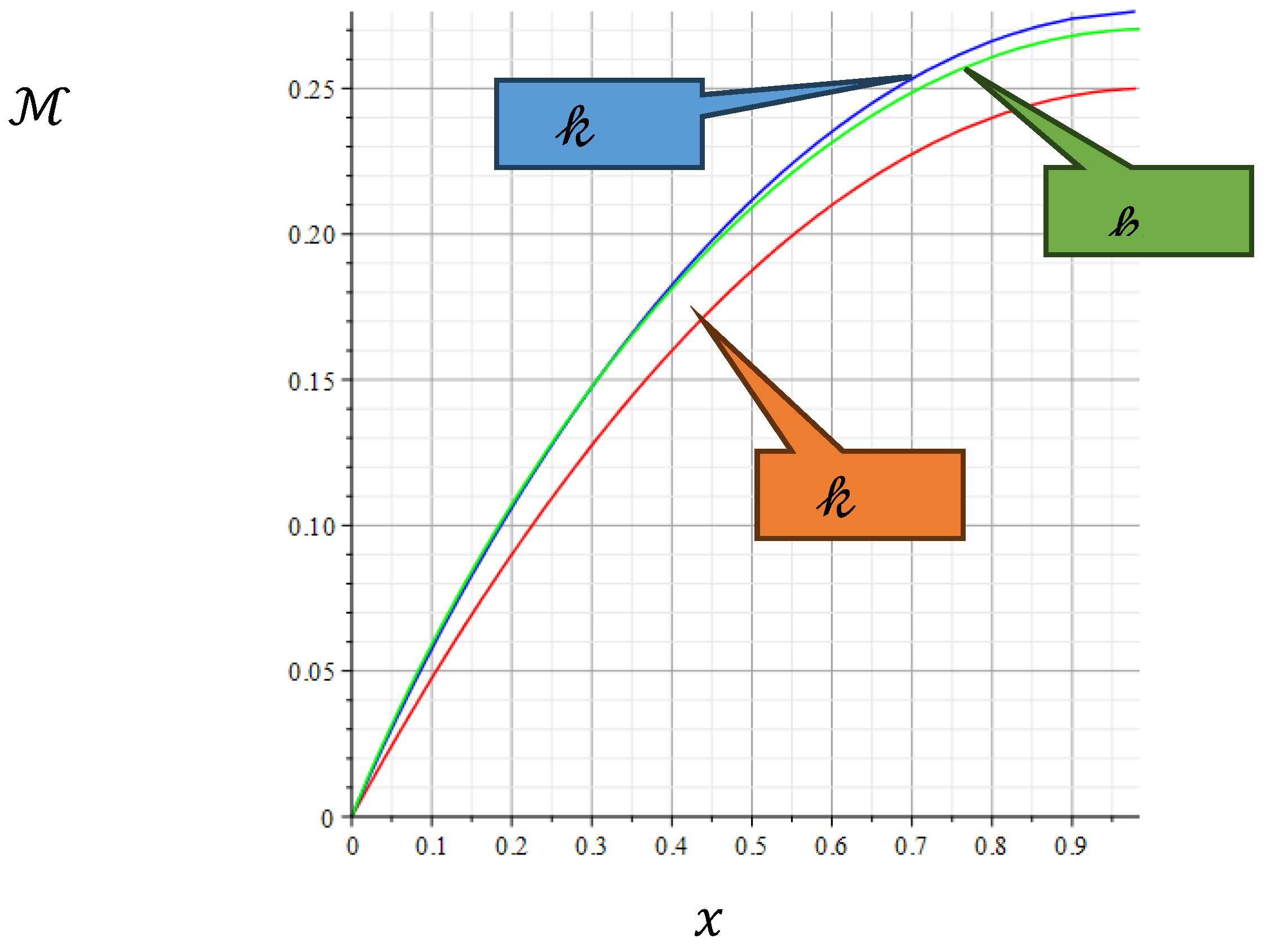
Figure 2.
Dimensionless function
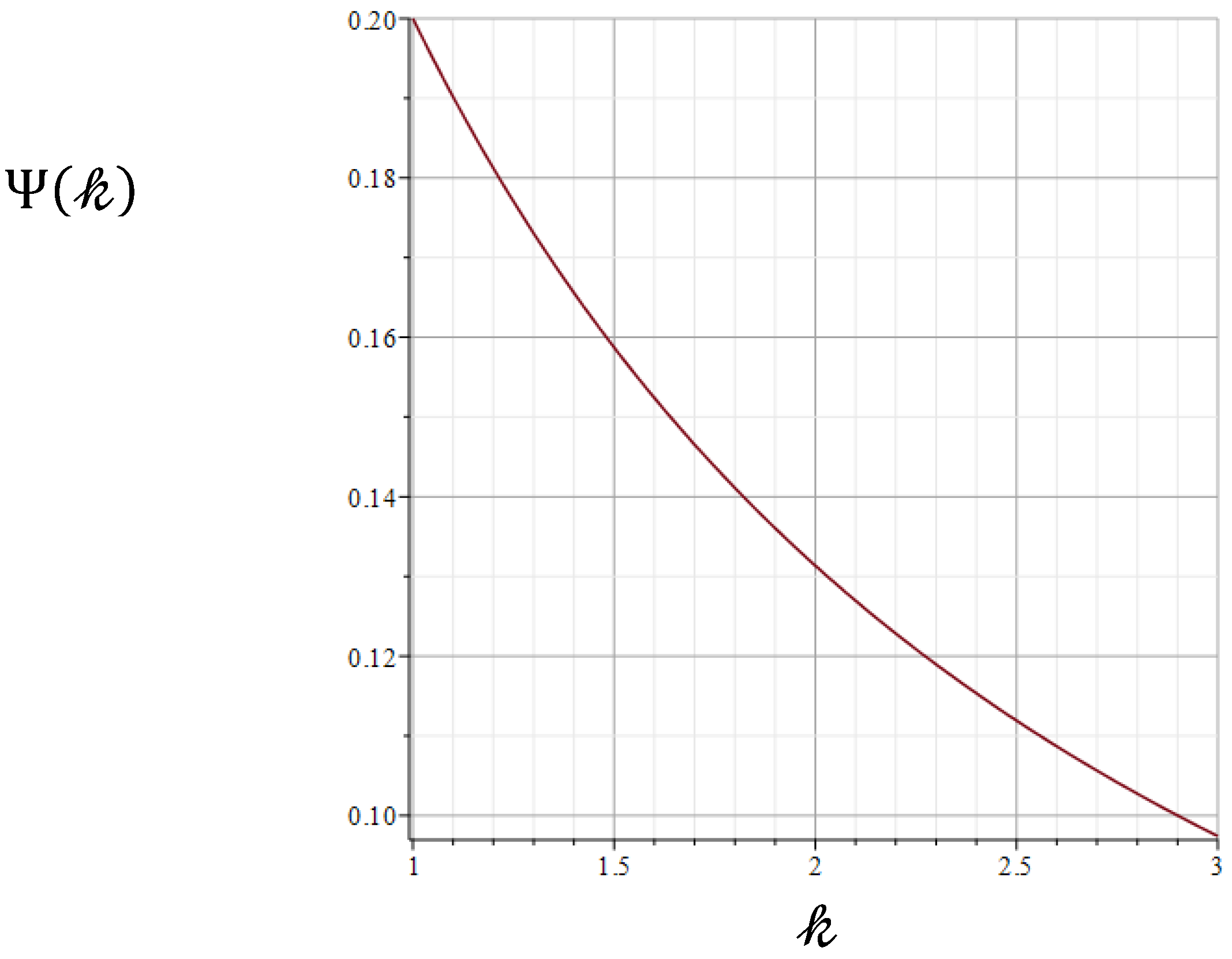
Figure 3.
as function of length and shape factor
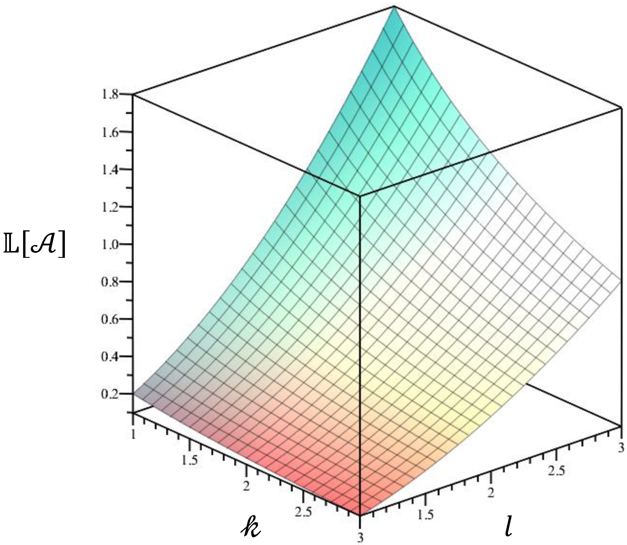
Figure 4.
Optimal shapes of twisted rods for the Nash equilibrium states.
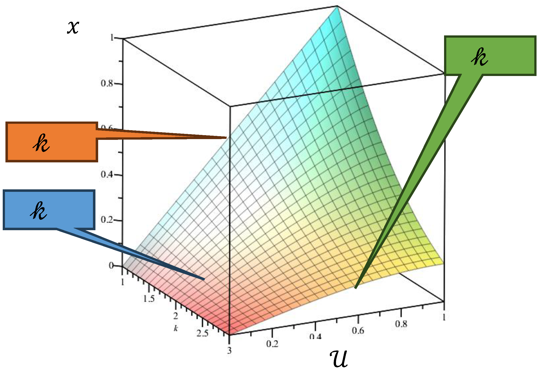
Figure 5.
Pareto fronts for the states of Nash equilibrium for different shape factors.
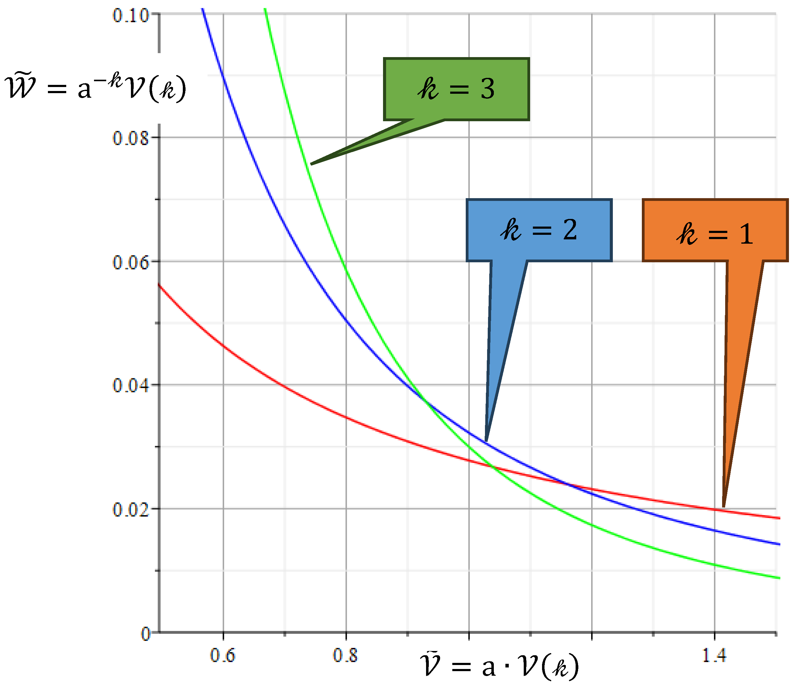

Table 1.
Areas, area moment of inertia and shape factors for the similar variation of the cross-section
Table 1.
Areas, area moment of inertia and shape factors for the similar variation of the cross-section
| Solid or (filled) cross section | equilateral triangle | regular hexagon | square | circular area |
|---|---|---|---|---|
| side length of | radius | |||
| area | ||||
| area moment of inertia | ||||
| shape factor | ||||
Table 2.
Expressions for axial coordinate as the function of for and
| 1 | |
| 2 |
Table 3.
Stored elastic energy and volume for Nash equilibrium
| 1 | |||
| 2 | |||
| 3 |
Table 4.
Expressions for axial coordinate as the function of for ,
| 1 | 1 | |
| 2 | ||
| 3 |
Disclaimer/Publisher’s Note: The statements, opinions and data contained in all publications are solely those of the individual author(s) and contributor(s) and not of MDPI and/or the editor(s). MDPI and/or the editor(s) disclaim responsibility for any injury to people or property resulting from any ideas, methods, instructions or products referred to in the content. |
© 2024 by the authors. Licensee MDPI, Basel, Switzerland. This article is an open access article distributed under the terms and conditions of the Creative Commons Attribution (CC BY) license (http://creativecommons.org/licenses/by/4.0/).
Copyright: This open access article is published under a Creative Commons CC BY 4.0 license, which permit the free download, distribution, and reuse, provided that the author and preprint are cited in any reuse.


