1. Introduction
Hyperspectral imaging has emerged as a keystone technology in remote sensing, where the ability to discern variations between high-resolution spectra supports a plethora of critical applications such as environmental monitoring, biodiversity conservation, sustainable agriculture, and more. In recent years, many remote sensing platforms have been deployed with hyperspectral imaging payloads such as the Italian PRISMA mission launched in 2019, the German EnMAP launched in 2022, and recently NASA’s PACE satellite launched in 2024 [
1,
2,
3]. Many future missions also plan to incorporate hyperspectral imaging capabilities such as the European Space Agency’s CHIME which will include over 200 bands spanning visible, near-infrared (NIR), and short-wave infrared (SWIR) wavelengths [
4]. The continued development of hyperspectral imaging technology has also led to a considerable reduction in size that enables its inclusion in the payloads of small unmanned aerial vehicles (UAVs) [
5,
6]. Despite the proliferation of hyperspectral imaging data sources, the considerable increase in data volume associated with hyperspectral images (HSI) poses significant challenges to real-time analysis at scale.
Many approaches have been developed to make sense of the HSI data. For example, spectral indices such as the popular normalized difference vegetation index (NDVI) can be computed by taking ratios of spectral bands tailored to track specific reflectance characteristics [
7,
8]. These indices have the advantage of being easy to compute, but suffer from significant variability between instruments while ignoring most of the information captured in HSI spectra [
9]. An alternative approach is to pair HSI data with in situ measurements to enable supervised models that map spectra directly to parameters of interest. However, this approach relies on serendipitous satellite overpasses above sensing sites to generate sufficient quantities of aligned data for model training and evaluation. For example, Aurin et al. combined data from over 30 years of oceanographic field campaigns with paired satellite imagery to develop robust models for the inversion of key water quality indicators such as colored dissolved organic matter [
10]. This approach can be accelerated by combining UAV-based hyperspectral imaging with rapid in situ data collection using autonomous boats [
11,
12]. However, these supervised methods rely on
a priori knowledge of expected sources to identify appropriate reference sensors for data collection. In light of these limitations, unsupervised methods are needed which can reliably extract source signatures from high-dimensional HSI.
The spatial resolution of hyperspectral imagers generally results in pixels with mixed signals from multiple sources called endmembers. The task of unsupervised source identification using HSI data therefore involves two steps: endmember extraction and abundance estimation. Techniques such as vertex component analysis (VCA), the pixel purity index (PPI), and N-FINDR solve this first task by identifying HSI endmember spectra assuming the presence of some pure (unmixed) pixels [
13,
14,
15]. By further assuming a linear mixing model (LMM) in which observed spectra are described by a linear combination of endmembers with non-negative abundances, HSI can be unmixed using a variety of techniques such as constrained least squares [
16,
17]. Among these methods, Nonnegative Matrix Factorization (NMF) is a widely used approach which extracts endmember spectra and unmixes abundances simultaneously via matrix factorization [
18,
19,
20]. The update equations for NMF can be formulated as multiplicative updates which guarantee the non-negativity of endmember spectra and their associated abundances [
21]. For this reason, the continued development of new NMF varieties remains an active area of research.
In realistic scenes, multiple scattering and surface variability can easily challenge the assumption of linear mixing [
22]. Water-based HSI specifically are prone to non-linear mixing effects due to absorption features of dissolved and suspended substances, fluorescence of organic matter, and particulate scattering in turbid waters [
23,
24,
25]. With the growing popularity of deep learning approaches in remote sensing, a variety of models based on autoencoder architectures have been introduced for unmixing HSI data [
26,
27,
28,
29]. However, the complexity introduced by these models significantly impacts training time and decreases the interpretability of the resulting model. An ideal approach should enable both endmember extraction and non-linear unmixing while accounting for spectral variability.
The self-organizing map (SOM) is an unsupervised machine learning method that maps high-dimensional data to a low-dimensional grid while preserving the topological relationships between data points [
30]. This low-dimensional representation provides a convenient way to visualize HSI data while the weight vectors for each SOM node can be interpreted as representative spectra [
31,
32,
33]. If labelled reference spectra are available, the SOM can be used to enable semi-supervised labeling of HSI pixels [
34]. The SOM has also been shown to be effective for the compression of HSIs acquired by a CubeSat [
35]. Despite these capabilities, the SOM does not offer a probabilistic interpretation and relies on a heuristic training procedure with hyperparameters that can be challenging to tune. To address these shortcomings, Bishop et al. introduced the Generative Topographic Mapping (GTM), a probabilistic latent-variable model inspired by the SOM [
36]. When choosing a two-dimensional latent space, the GTM can be used to visualize the distribution of HSI spectra while mapping the latent space nodes to the HSI data space provides endmembers [
37]. Unfortunately, the rectangular latent space grid employed by the GTM does not directly translate into endmember abundances, and the expectation-maximization (EM) algorithm used to train the GTM does not guarantee non-negativity of GTM node spectra.
In this paper, we introduce a new variant of the GTM dubbed Generative Simplex Mapping (GSM), which can extract endmember spectra and unmix non-linear mixtures. By replacing the rectangular latent space of the GTM with a gridded -simplex, the vertices of the GSM can be immediately interpreted as endmembers corresponding to n unique spectral signatures. The mapping from the latent space to the HSI data space models signal mixing while barycentric coordinates for the latent space simplex represent relative endmember abundances. Additionally, by taking inspiration from the multiplicative updates of NMF, the GSM algorithm maintains the non-negativity of resulting endmember spectra. If only linear mixing is present, the GSM algorithm drives non-linear contributions to 0. Prior distributions included for GSM model weights yield hyperparameters which can be tuned to control the smoothness of the resulting spectra and the degree of non-linear mixing applied.
The remainder of the paper is structured as follows.
Section 2 describes the proposed method.
Section 3 and
Section 4 describe experiments using simulated and real HSI data to evaluate the GSM model.
Section 5 discusses additional applications and extensions of the GSM to be explored in future work. Finally,
Section 6 finishes the paper with some closing remarks.
2. Generative Simplex Mapping
In the original GTM formulation, the data vectors
(reflectance spectra) are described by latent variables
mapped into the data space by a non-linear function
. The data space distribution is taken to be normal with the precision parameter
to account for measurement noise and spectral variability. The GSM uses same structure, that is
where
are model weights which parameterize the mapping
.
Assuming data are uniformly sampled from an embedded manifold in the data space, the GTM models the latent space using a rectangular grid with
K-many nodes of equal prior probability. To adapt the GTM to describe endmember mixing, the GSM makes two key changes. The first is to replace the rectangular GTM grid with a gridded simplex with
vertices. The barycentric coordinates for each node then describe the relative abundance of each endmember with each vertex corresponding to a pure endmember. The second change is to replace equal prior probabilities with adaptive mixing coefficients
to allow the GSM to model HSI with nonuniform mixing distributions. Together, this leads to a latent space prior distribution given by
For a data set containing
N-many records, these definitions yield a log likelihood function given by
which can be maximized to obtain optimal values for model weights
, mixing coefficients
, and precision
. Rather than optimizing Equation (
3) directly, we instead choose a particular form for
to allow fitting the GSM via an EM algorithm.
In the standard LMM model, the mapping
is given by
where the columns of
correspond to endmember spectra. To model non-linear mixing,
is replaced by the output of
M-many activation functions such that
. The activations applied to each GSM node can then be collected to form a matrix with elements
. For
, we take
to model linear mixing. The remaining
activations are computed using radial basis functions (RBF) with centers
distributed throughout the simplex (but not at the vertices) with
where
s is the spacing between RBF centers. In this form, the first
columns of
correspond to endmember spectra, while the remaining columns account for additional non-linear effects. For linear mixing, the GSM training algorithm should therefore drive
to 0 for
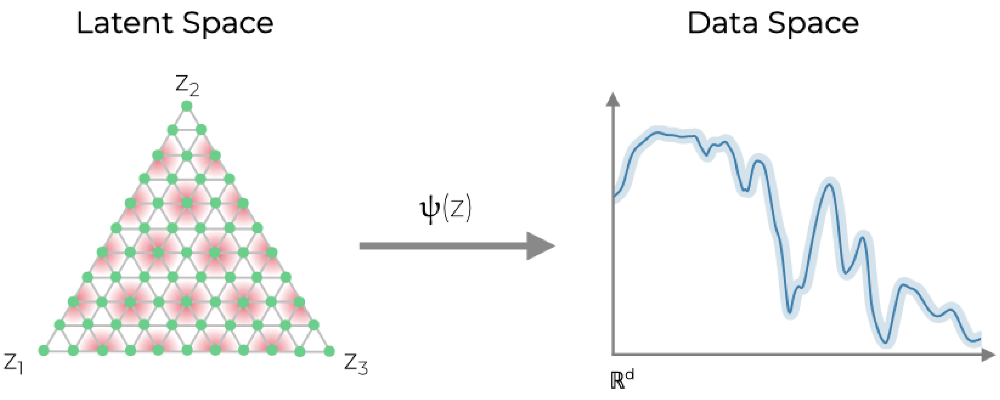
. A visualization of the GSM model is shown in
Figure 1.
To further constrain the model, we introduce prior distributions on the weights . For we take corresponding to a zero-mean Gaussian with variance . For we use a zero-mean Laplace distribution, , with scale parameter . Under these choices corresponds to regularization on endmember spectra while corresponds to regularization on the non-linear activations. In other words, governs the smoothness of the resulting endmembers while encourages sparsity for the non-linear contributions.
An EM algorithm for the GSM model can now be formulated as follows. Suppose that we have current estimates for the model weights
, mixing coefficients
, and precision parameter
. During the expectation step we compute the posterior probabilities, that is, the responsibility of each GSM node for each spectrum in the data set:
For the maximization step, we consider the expectation of the penalized complete-data log likelihood given by
where
is the
d-th component of the
n-th spectrum in the data set. Equation (
6) is then maximized with respect to
,
, and
to obtain new parameter values. For a detailed overview of the EM procedure, the reader is directed to ref. [
38].
For
, optimization can be performed using Lagrange multipliers to maintain the condition that
. Doing so yields
Optimization of Equation (
6) with respect to
leads to a linear system which can be solved using standard numerical methods. However, in this form, we cannot guarantee the non-negativity of
required to describe reflectance spectra. Therefore, we take inspiration from the multiplicative updates for NMF introduced by Lee and Seung [
18]. A standard gradient-based update for
would normally take the form
for some learning rate
. Therefore, we differentiate to obtain
where
is a diagonal matrix with
and
is given by
If we allow individual learning rates
for each element of
, then choosing
results in a multiplicative update rule given by
From Equation (
12), it is clear that we are multiplying
by strictly non-negative values, and therefore, non-negative
will remain so during each update. This update can also be repeated multiple times during each M-step to accelerate convergence.
Optimizing Equation (
6) with respect to
yields the final update equation:
To train a GSM model, weights
are randomly initialized to positive values. The mixing coefficients are initially set to
. Finally, the precision parameter
is initialized to the variance of the
-th principal component. After initialization, the expectation and maximization steps are repeated in turn until
Q converges to a predetermined tolerance level. For large
we note that generating a regular grid within the simplex becomes cumbersome as the number of grid nodes scales as
for
k nodes per edge. An alternative approach is to randomly sample points within the simplex to obtain a total of
K nodes. A Dirichlet distribution
with all
can be used to uniformly sample within the simplex. Since the mixing coefficients
are adaptive, variability in node separation should not significantly impact the resulting GSM.
The probabilistic form of the GSM means that a variety of information criteria can be used to evaluate the model fits. In this paper we consider two metrics, the Bayesian Information Criterion (BIC),
and the Akaike Information Criterion (AIC),
where
P is the total number of model parameters and
is the log likelihood from Equation (
3).
The map
provides the representation of each node
in the data space. Importantly, applying
to each vertex extracts endmember spectra from the GSM. Slices
of the matrix
define the responsibility of each latent node
for the
n-th spectrum
in the data set. Therefore once the GSM has been trained,
can be used to unmix endmember abundances by representing each record in the latent space via the mean:
A freely available implementation of the GSM is provided at [
39]. The code is written in the Julia programming language and follows the Machine Learning in Julia (MLJ) common interface [
40,
41].
5. Discussion
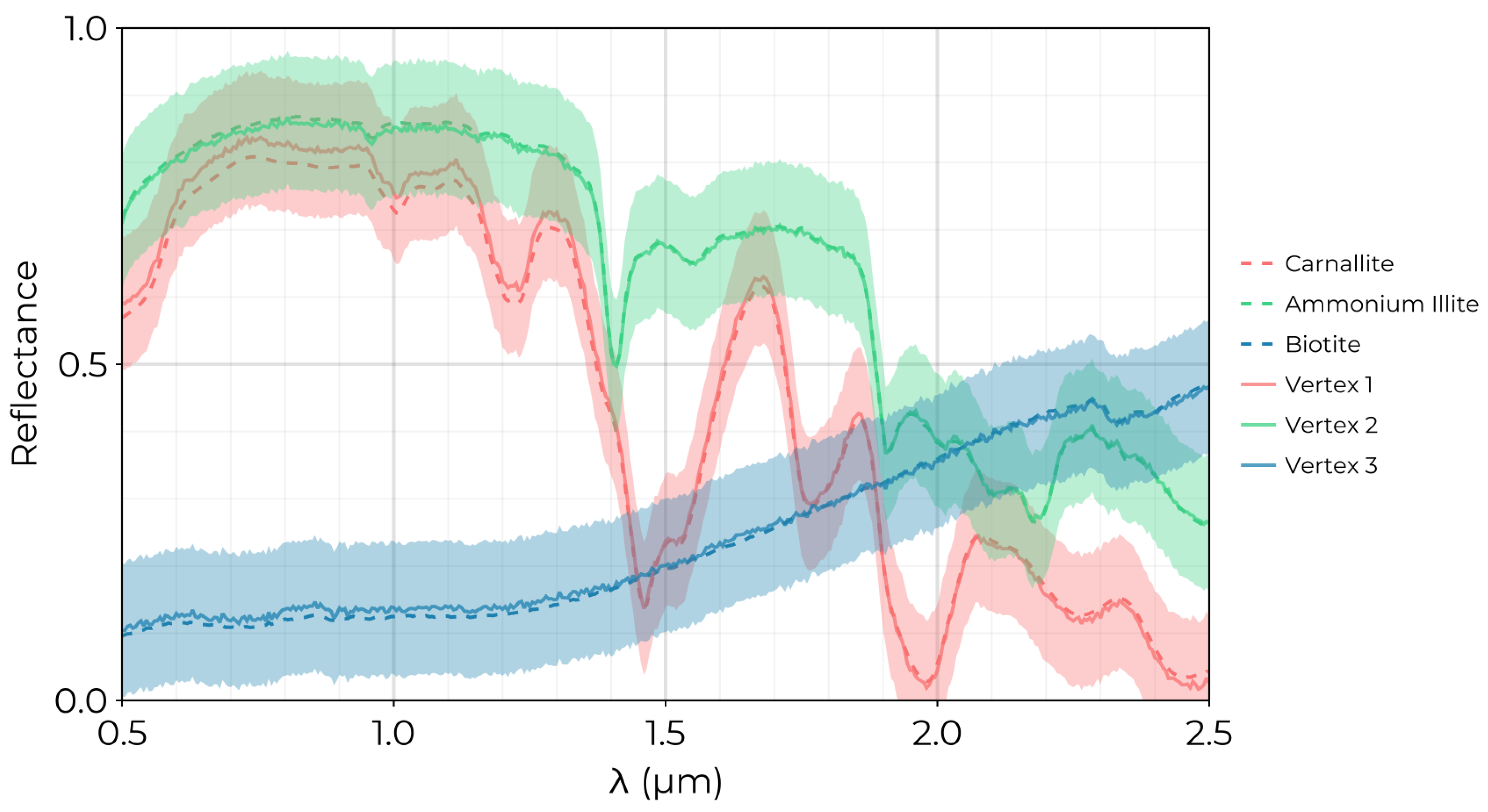
The proliferation of hyperspectral imaging technologies in the remote sensing and environmental monitoring communities underscores the need for efficient algorithms that can make sense of high-dimensional HSI. Of particular interest are unsupervised algorithms which utilize all available wavelength bins to identify unique source profiles that present realistic scenes. The GSM introduced in this paper is a novel method that simultaneously performs endmember extraction and spectral unmixing. Unlike popular endmember extraction algorithms, such as VCA, PPI, and N-FINDR, GSM does not assume the presence of pure pixels in HSI. Furthermore, the flexible structure of the mapping from the GSM latent space to the spectral data space allows the GSM to model non-linear mixing effects, distinguishing it from other widely used linear models such as NMF. Being a probabilistic model also enables the GSM to quantify the spectral variability through the precision parameter
as indicated in
Figure 6. This additional capability is critical for analysis of realistic HSI where sensor noise, viewing geometry, and scene illumination all introduce uncertainty into extracted endmembers.
The growing popularity of deep learning methods has led many to explore applications of deep learning to the spectral unmixing problem. Variations in auto-encoder architectures are a popular choice for both endmember extraction and unmixing. For example, Borsoi et al. used a variational autoencoder to more accurately identify the spectral variability in a LMM [
28]. Similarly, Palson et al. introduced an autoencoder with convolution layers to extend the LMM by incorporating spatial context from neighboring HSI pixels [
29]. However, the increased complexity of deep neural network approaches makes interpreting the latent space learned by encoder layers challenging and can dramatically increase training time and data volume requirements. In contrast, the latent space of the GSM is immediately interpretable due to the imposed simplex geometry, while the form of
leaves room to explore a variety of non-linear mixing models. In this paper,
was constructed to add non-linear effects as additions or perturbations to an underlying linear mixing model with the
hyperparameter provided to control the degree of non-linearity considered. In the original GTM formulation that inspired the GSM, the mapping
strictly uses non-linear features generated by Gaussian RBFs. Alternatively, one could easily construct
for specific non-linear models such as bilinear mixing by introducing features which depend on higher-order combinations of the latent space (abundance) coordinates. However, it is important to note that the EM algorithm formulated for GSM training is made possible due to the linear combination of activations
with model weights
. For mixing models which instead depend non-linearly on weights
, an EM algorithm may require iterative non-linear solves during each M step.
The main limitation of the GSM is the curse of dimensionality encountered when generating a grid on the
-simplex for large numbers of endmembers,
. This can be mitigated by instead randomly sampling points within the interior of the simplex using a uniform Dirichlet distribution to obtain a pre-determined number of nodes across the latent space. As the mixing coefficients
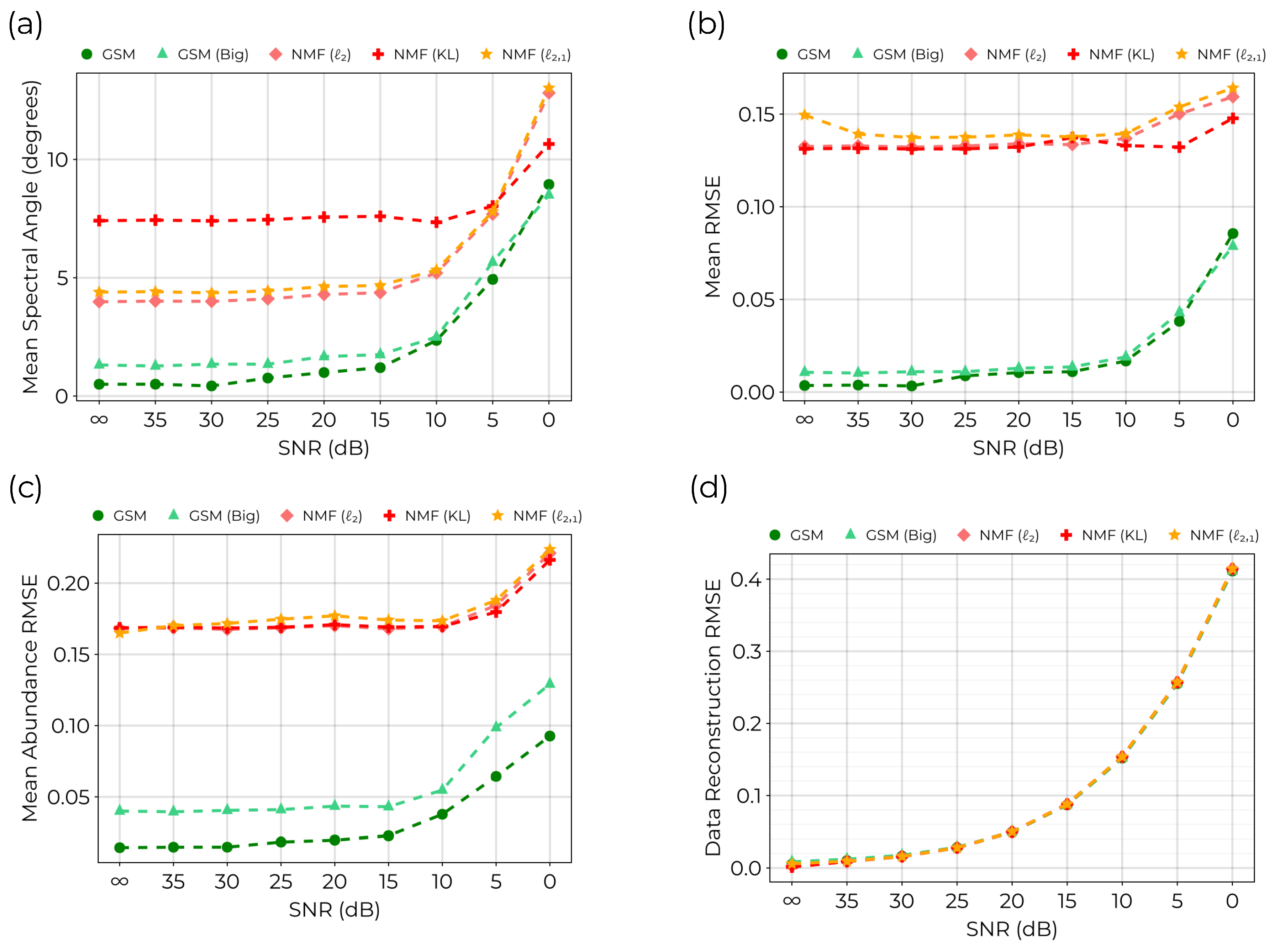
are adapted during training, the variability in the spacing of the internodes should not significantly affect the performance of the model. In fact, this was confirmed for the simulated data set as summarized in
Figure 5. For considerably large data sets, the size of the responsibility matrix
can also lead to extended training times. This can be addressed by augmenting the EM procedure to updated using mini-batches of training samples during each E-step as described by Bishop et al. for the GTM in ref. [
47]. Rather than updating the full responsibility matrix, a subset of
corresponding to a single batch of training data can be evaluated with all other entries kept constant. The GSM may also be extended in other ways, for example, by replacing the precision parameter
with a covariance matrix to model wavelength-dependent spectral variability common to many hyperspectral imaging platforms.
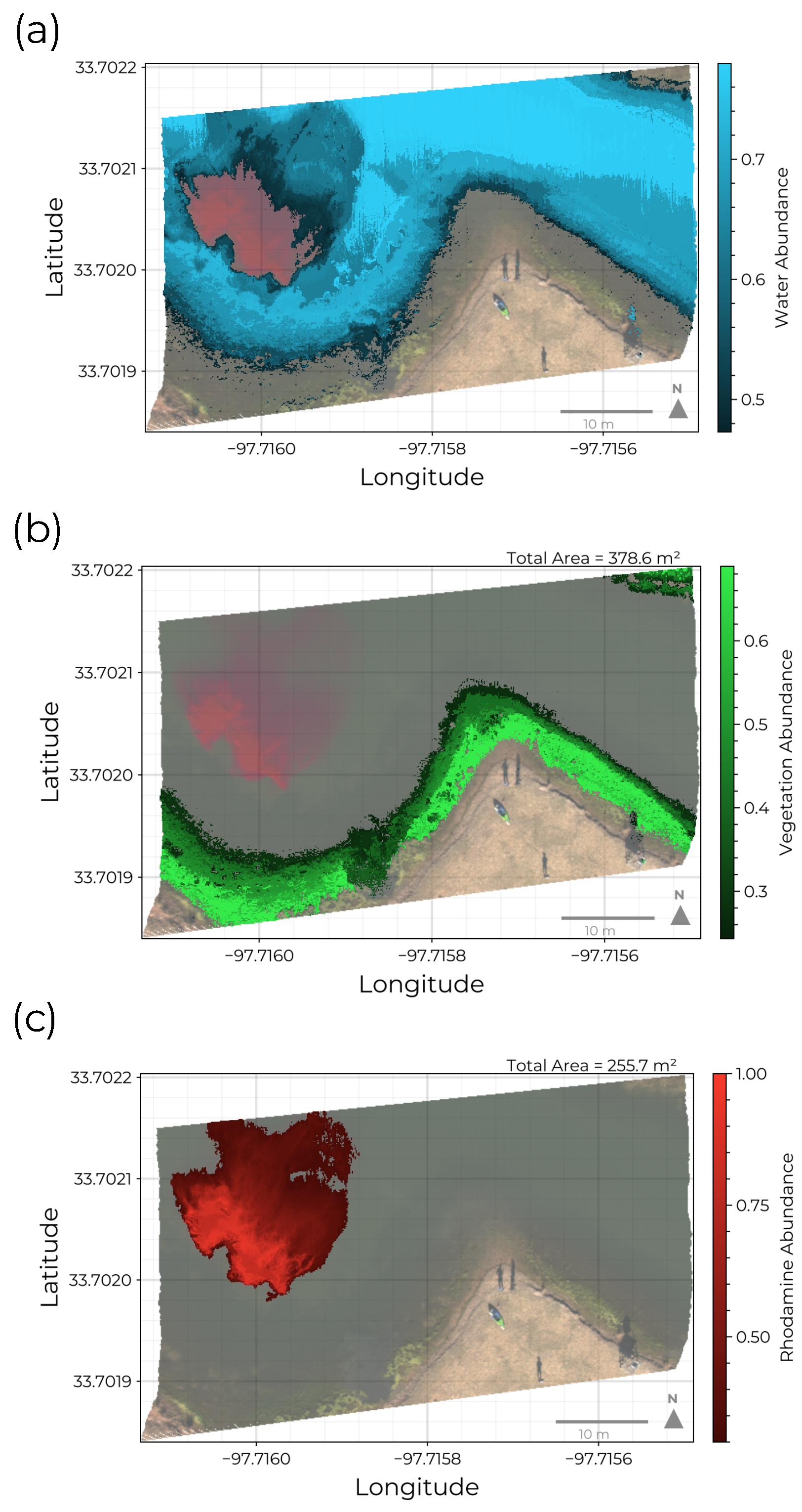
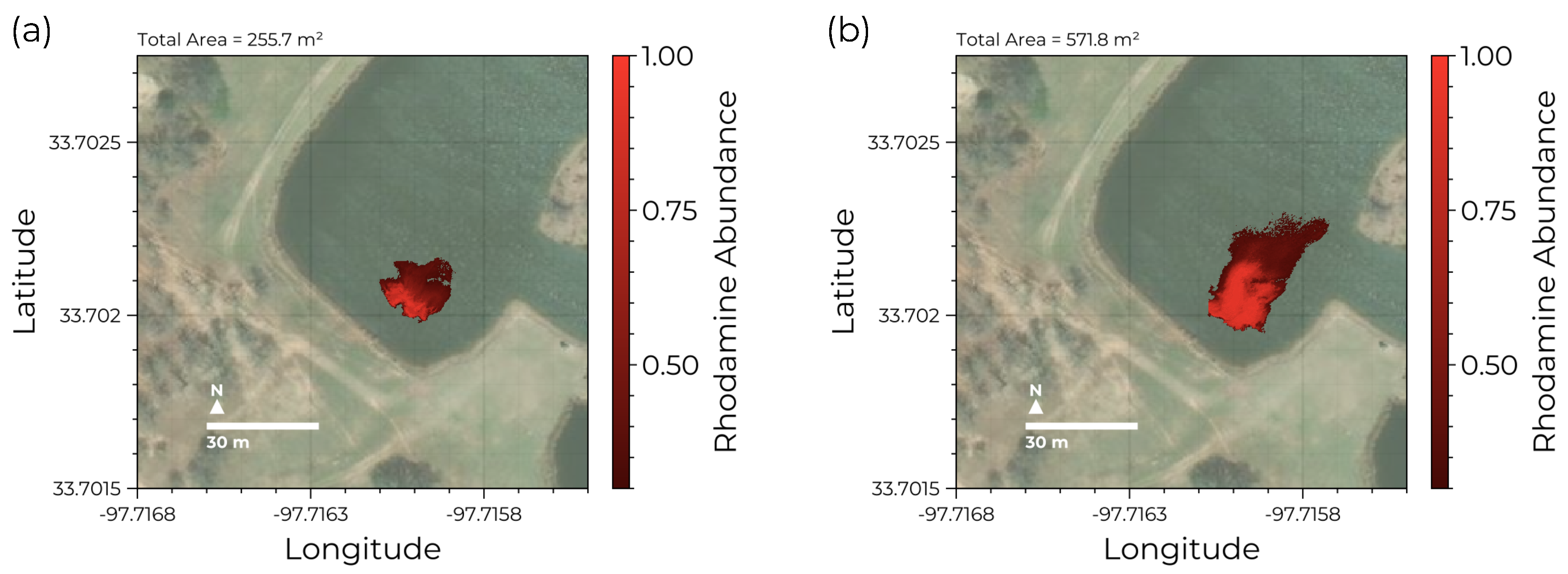
Based on the results of applying the GSM to real HSI as illustrated in
Figure 8 and
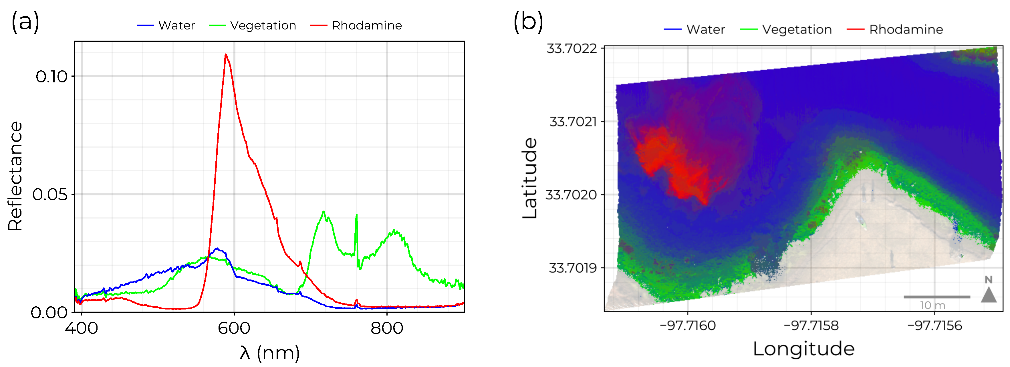
Figure 9, one clear application of the GSM is to contaminant identification and water quality assessment. Modern UAV platforms make it possible to rapidly image bodies of water where direct access for in-situ data collection is restricted. By equipping UAVs with hyperspectral imagers, the GSM can be used to identify abnormal spectral signatures corresponding to localized contaminant sources. Generating semantic segmentations of collected HSI as in panel b of
Figure 7 makes it easy to compare multiple HSI without resorting to pseudocolor images generated from a limited number of wavelength bands. Since the GSM models the distribution of all HSI spectra rather than individual parameters, it may also aid in-situ data collection by suggesting sampling points which maximize the area traversed in the GSM latent space rather than uniformly sampling across a wide spatial extent. Similar approaches have been developed to guide autonomous data collection vehicles by casting route planning as a prize collecting travelling salesman problem subject to resource constraints [
48,
49].
As a final consideration, we note that the problem of endmember extraction and spectral unmixing for HSI is identical to source apportionment in the context of air quality. Here, the goal is to identify measurement profiles associated with sources of ambient air pollution based on measurements at a receptor site. A popular model for source apportionment studies is Positive Matrix Factorization (PMF) introduced by Paatero and Tapper [
50,
51]. Just like NMF, PMF decomposes measurements into a convex combination of source profiles and relative abundances subject to non-negativity constraints. These linear receptor models assume that the sources are not transformed during transport to the receptor, ignoring changes due to chemical reactions. Non-linear mixing models such as the GSM introduced here may, therefore, prove beneficial in this additional domain.
Figure 1.
Illustration of the GSM. The latent space consists of a grid of K-many points (green dots) distributed throughout a simplex with vertices. Barycentric coordinates of each node in the simplex correspond to the relative abundance of -many unique sources. Here, has been chosen for illustrative purposes. Nodes are mapped into the data space via the map utilizing M-many radially symmetric basis functions (red). Spectral variability is estimated via the precision parameter shown here in the data space as a light blue band around the spectrum given by .
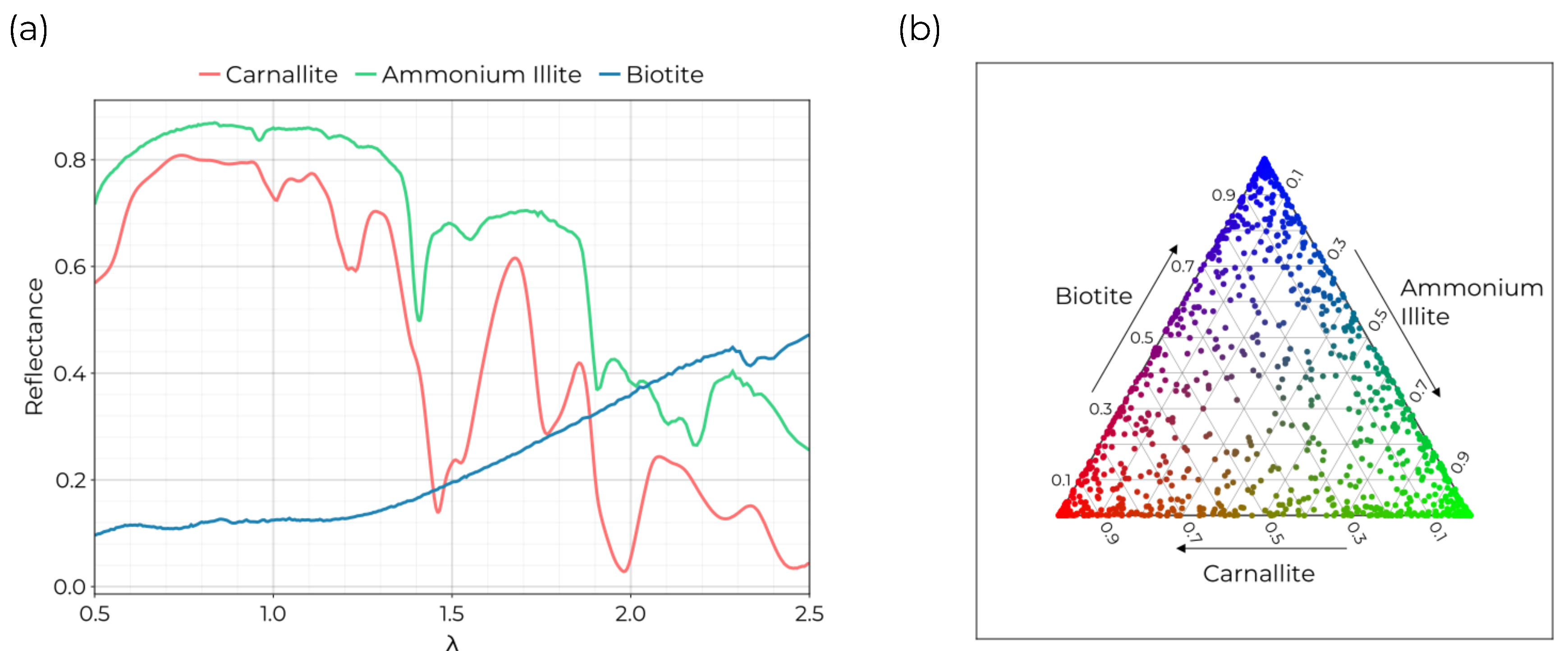
Figure 2.
Synthetic data set formed from USGS spectra.
(a) Spectra from the USGS spectral database used as the ground truth endmembers. These spectra were selected following the example in ref. [
13].
(b) The abundance distribution sampled for in the data set. Samples were generated from a Dirichlet distribution with
.
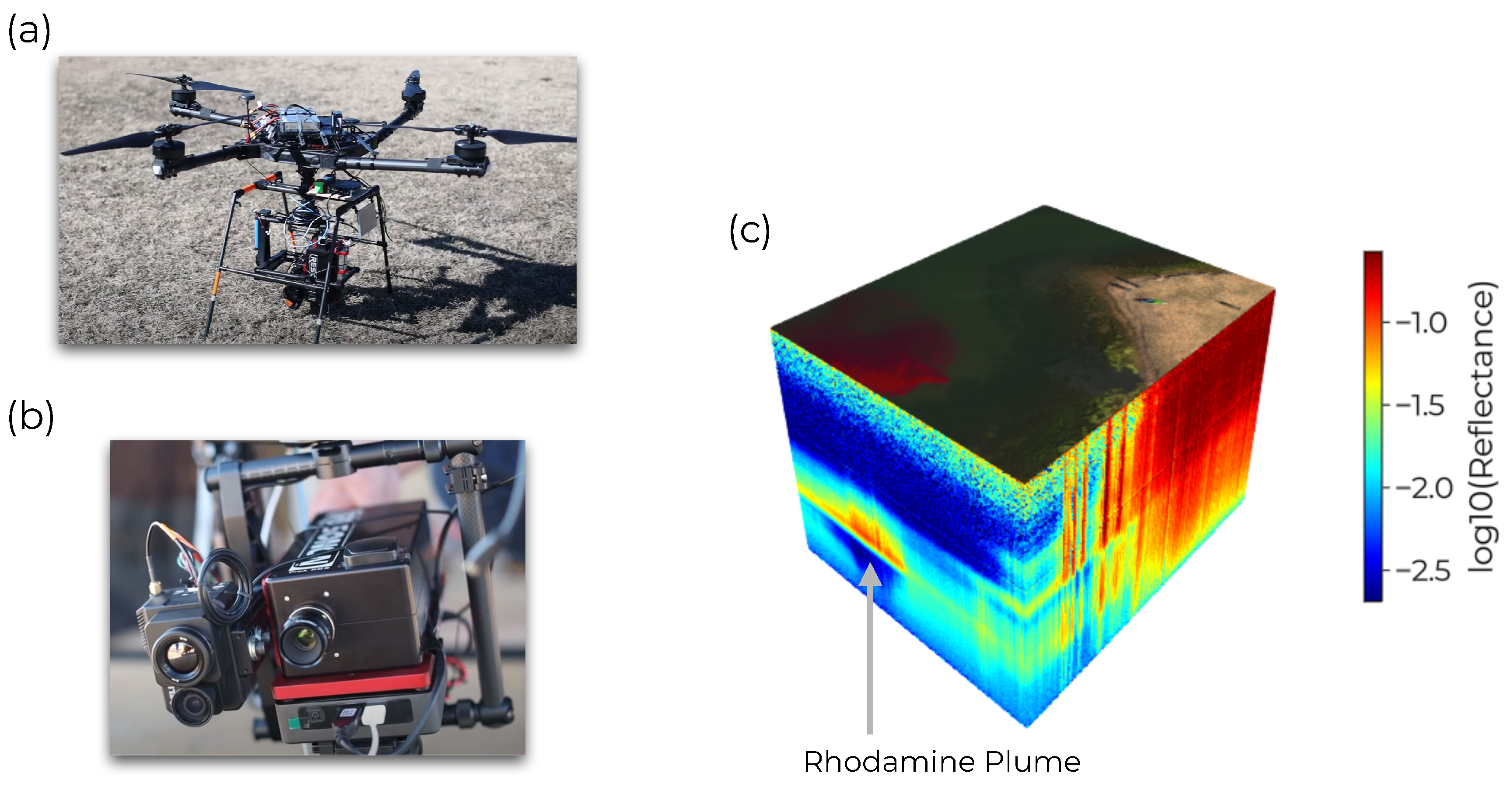
Figure 3.
Real HSI Data set. (a) the UAV used to collect hyperspectral images. (b) The Resonon Pika XC2 hyperspectral imager used to acquire HSI. (c) A sample hyperspectral data cube. Spectra a plotted using at their geographic position with the log10-reflectance colored along the z axis and a pseudocolor image on top. The signature of the rhodamine dye plume is clearly identifiable in the water.
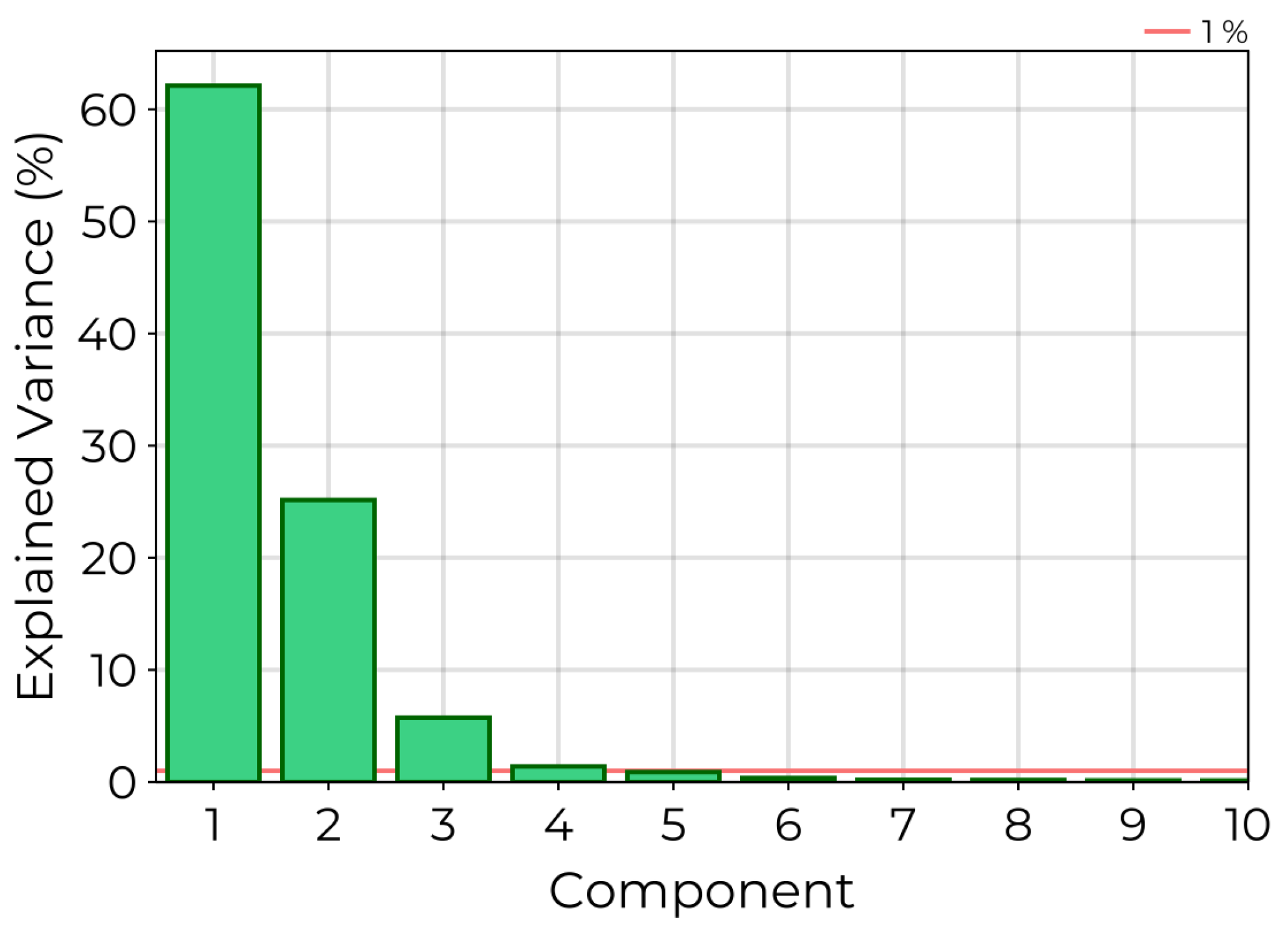
Figure 4.
Explained variance of PCA components for the real HSI data set. A red horizontal line is superimposed on the graph, marking an explained variance of . All components past the fourth explain less than of the observed variance.
Figure 4.
Explained variance of PCA components for the real HSI data set. A red horizontal line is superimposed on the graph, marking an explained variance of . All components past the fourth explain less than of the observed variance.
Figure 5.
Comparison of GSM against NMF on simulated linear mixing data set using USGS spectra. (a) The mean spectral angle computed between extracted endmembers and original endmembers. (b) the mean RMSE computed between extracted endmembers and original endmembers. (c) The mean abundance RMSE computed between original abundance data for each endmember and extracted abundances. (d) The reconstruction RMSE which evaluates the quality of fit. All models realized similar values reflecting convergence of the models to the level of random noise introduced into the data.
Figure 6.
Endmembers extracted by the GSM for the simulated linear mixing data set with SNR. The dashed lines correspond to original endmember spectra from the USGS spectral database. Solid lines superimposed on the plot indicate the extracted endmember spectra. Colored bands are included around each spectrum corresponding to the spectral variability estimated by the GSM precision parameter where the band width is corresponding to 2 standard deviations.
Figure 7.
GSM applied to water spectra from real HSI data set: (a) Spectra generated by the trained GSM for samples with maximum abundance for each endmember. Based on these spectral profiles, endmembers are identified with water, near-shore vegetation, and rhodamine dye. (b) A HSI segmented according to the relative abundance of each endmember. Each water pixel is colored by smoothing interpolating between red, green, and blue colors using the relative abundance estimated for rhodamine, vegetation, and water spectra. The rhodamine plume is clearly identifiable in the western portion of the HSI.
Figure 8.
Endmember abundance distributions: (a) The spatial distribution of abundance for the water class. This source dominates in the center of the pond and decreases towards the shore where vegetation begins to dominate the reflectance signal. The water endmember abundance is also observed to decreases near the edge of the rhodamine plume reflecting dye mixing and diffusion. (b) The spatial distribution of vegetation. This endmember includes filamentous blue-green algae observed to accumulate in shallow waters near the shore. (c) The rhodamine dye plume extent segmented from the HSI. The total area for near-shore vegetation and rhodamine are estimated to be and , respectively.
Figure 9.
Rhodamine plume evolution: Using the trained GSM we can track the dispersion of the rhodamine dye plume between successive drone flights. (a) The initial plume distribution after release. Here the dye subsumes an area of . (b) The same plume imaged 15 minutes later now extends across an area of
Table 1.
GSM hyperparameter optimization for the real HSI data set: Multiple GSM models were trained to explore the impact of model hyperparameters. values from 3 to 6 were explored as suggested by the PCA decomposition of the data set. was varied from to and ranged from 1 to 1000. Here we report the top 10 models ranked by increasing BIC. The AIC and reconstruction RMSE are also included for comparison.
|
|
|
BIC |
AIC |
Reconstruction RMSE |
| 3 |
|
|
|
|
|
| 3 |
|
|
|
|
|
| 3 |
|
|
|
|
|
| 3 |
|
|
|
|
|
| 4 |
|
|
|
|
|
| 4 |
|
|
|
|
|
| 4 |
|
|
|
|
|
| 4 |
|
|
|
|
|
| 4 |
|
|
|
|
|
| 3 |
|
|
|
|
|
