
Submitted:
29 September 2024
Posted:
15 October 2024
You are already at the latest version
Abstract
This study aims to investigate the dynamic impact of socio-economic issues such as youth unemployment and income inequality on crime by comparing the findings from newly democratized African countries (South Africa and Namibia) to those of recently democratized European countries (Lithuania and the Ukraine) and newly democratized Asian countries (Kyrgyzstan) from 1994 to 2019.
The study used the Bayesian vector autoregression approach with hierarchical priors. This model was chosen due to its ability to address the dynamics of several entities, such as the measurable defects where data quality is uncertain, or perhaps lacking as frequently happens. Prior selection in a Bayesian vector autoregression approach can help adjust for these flaws. According to the study's findings, an unexpected shock in unemployment and income inequality has a significant positive impact on crime; however, an unanticipated shock in government expenditure has a significant negative impact. The results are interesting, as we found that the impact of these socio-economic issues does not necessarily depend on the geographical area, as the results are similar for income inequality in both regions. This study serves as a wake-up call to the government that some policies (fiscal policy or income policy) are more appropriate for resolving concerns about inequality and unemployment than others. As a result, addressing these issues through policies that promote greater economic equality and ensure everyone has access to basic education, healthcare, and job training, could assist in reducing crime while promoting a more equal society.
Keywords:
Africa
; Asia
; BVAR
; crime
; Europe
; income inequality
; newly democratized countries
; unemployment.
1. Introduction and Background of the Study
For decades, criminal activity has been a serious socioeconomic concern that has caught the attention of every corner of the world. As countries attain independence, there is considerable concern about whether governments and societies’ policies and behaviours will be sound enough to regulate these issues (violence, unemployment, and income inequality). A further concern was that criminal activity would increase as people transitioned from traditional to contemporary ways of living, so that they could experience socioeconomic and cultural changes. In an attempt to address such concerns, we aim to investigate the impact of unemployment and income inequality on crime in newly democratised African countries and further compare these findings with those of newly democratised European countries.
Newly democratized countries face numerous socioeconomic challenges, including economic instability, deep-seated inequality, corruption, limited access to education and healthcare, and a lack of experience in governance and civil society engagement. These issues can hinder growth and development, exacerbating tensions between social classes and ethnic groups. Corruption can undermine public trust in democratic institutions, and limited access to education and healthcare can restrict social mobility. To achieve sustainable democracy, these obstacles require careful navigation and support from domestic and international stakeholders.
The concept of "newly democratised" depends on the authors' definition and the study's objectives. However, the broad definition of newly democratised countries could be defined as those countries that gained independence from the 1950s to date. According to the board definition, there are 100 countries regarded as being newly democratised, of which 48 are African countries, 31 Asian countries, and 21 European countries. The current study aims to examine the dynamic impact of socioeconomic issues on crimes using a time series model. The aim is to trace the current level of socio-economic issues within newly democratised countries. To achieve this, the definition of newly democratised countries has been restricted to the 1990s, reducing the number of countries to six. These countries include South Africa and Namibia for African countries, the Ukraine and Lithuania for European countries, and Palau and Kyrgyzstan for Asian countries. However, with respect to the issue of data availability, we decided to drop Palau from Asia as there was data missing on this country. That means we have only one country for Asia while in the other regions we have two countries. The main aim of this study is to understand the dynamic impact of socio-economic issues on crimes in country-specific ways, rather than combining countries as in a panel study on newly democratised countries. Thus, the study aims to compare the results from African newly democratised countries to those of European and Asian newly democratised countries that became independent from the 1990s to date. The intuition is to study that which can be learned by newly democratised African countries from newly democratised European countries.
A brief explanation of when these countries got their independence from their oppressors: South Africa gained independence in 1910 but remained under British control under a white minority administration that imposed apartheid practices. In 1994, Nelson Mandela became the first black president, leading to South Africa’s complete independence. Namibia gained independence in 1990, with Dr Sam Nujoma as its first president. Lithuania declared independence in 1990, followed by the Ukraine’s declaration in 1991, which followed the laws of the Ukrainian SSR. Kyrgyzstan gained independence in 1991. These countries achieved independence from their oppressors through various means, such as wars, etc.
Figure 1 graphically demonstrates the mean Gini coefficient, youth unemployment, and crime covering the period (1994–2019) for newly democratised African countries, newly democratised European countries and an Asian country. We calculated a five-year average for all three socio-economic variables included in this study to trace how these socio-economic variables behave every five years.
The graph demonstrates that all these regions suffer most from high income inequality and, with the exception of the Asian region, all these countries suffer from huge problems of youth unemployment and crime. As much as there has been some improvement in mitigating these socio-economic issues in other countries such as Namibia, their level of these socioeconomics seems to be declining in 2014–2019.
The data show that crime rates, especially the murder rate, are high in countries with a high level of income inequality and unemployment (Zungu & Mtshengu, 2023). Given what the data is saying with respect to these socio-economic issues in these three regions, the current study seeks to empirically investigate the dynamic impact of the socioeconomics on crimes in newly democratised African countries and compare the findings with those of newly democratised European and Asian countries. The comparison will be made in order to find out whether this socio-economic problem depends on the country’s heterogeneity or on its demographics. All of these issues pose a slew of concerns, such as: whether youth unemployment is actually the root cause of criminal behaviour; whether there is a correlation between inequality in wealth and criminal activity; whether it is true that having legitimate employment lessens the desire to participate in criminal activity, and what policymakers can do to address these concerns?
Certain theories have produced contradictions on this subject, which then led to greater controversy over the empirical research on the impact of unemployment and income inequality on crime. Theories, such as Merton’s strain theory (1938), claim that failure to achieve financial success (often described by a lack of jobs) can frustrate people ranked low in the social structure owing to economic hardship, resulting in retaliatory crime. After three decades, Becker (1968), subsequently endorsed by Ehrlich (1975), examined this relationship from an economic point of view, which was fundamentally different from the strain hypothesis. Their logic is predicated on the idea that people commit crimes when the perceived benefits outweigh the consequences. According to economists, unemployment indicates a lack of legitimate jobs in the labour market. A lack of respectable work reduces the opportunity cost of committing a crime, driving people to engage in illicit activities. As a result, economists, unlike sociologists, believe that unemployment is positively related to crime. Another significant contribution to this topic may be found in the school of thought held by criminologists, who believe that unemployment is adversely related to crime. They contend that unemployment results in fewer crime victims and stolen goods (Cantor & Land, 1985, 2001).
The current study seeks to contribute to the existing literature by following the study documented by Zungu and Mtshengu (2023) in a panel of African emerging economies using the PVAR. Our study seeks to extend their work by control over the fiscal policy instances in the system, as government intervention through government expenditure plays a crucial role in reducing the impact of these socio-economic issues. Further contributions will be drowned out, given the concern that this socio-economic issue might be related to the country. Therefore, our study used Bayesian Vector Autoregression (BVAR) with hierarchical priors covering the period 1994–2019, due to data availability. We constructed the BVAR with hierarchical priors in response to two measurable defects: when the data quality is uncertain and when it is frequently short. Then, prior selection in a BVAR can help adjust for these flaws. Furthermore, the impulse response function is more exact when the present matter is estimated using Bayesian approaches. To further stress the study by Banbura et al. (2010), they argue that Bayesian vector auto-regression (BVAR) is a useful tool for large dynamic models due to its credibility, structural analysis, dynamic relationships, uncertainty accounting, modeling interdependencies, time-series analysis, and flexibility. Therefore, as in the current study, we are dealing with the dynamic impact of socioeconomic issues on crime. We believe that these kinds of issues have structural characteristics, which is why we find the BVAR to be suitable for this study. BVAR allowed for the simultaneous estimation of the effects of youth unemployment and income inequality on crime and was particularly useful in dealing with uncertainty in parameter estimation and further constructing the impulse response. This intends to investigate the dynamic impact of socioeconomic issues on crimes in African newly democratised countries and compare the results with those of European and Asian newly democratised countries. Precisely following the theoretical argument of the study, we have two socioeconomic variables, which are regarded as our dependent variables, with the aim of testing the impact of these socio-economic variables (income inequality and unemployment) on crime. Beyond these issues, the current study further seeks to expand the socio-economic crime definition by involving fiscal policy in determining the role played by fiscal policy in easing the impact of these socio-economic challenges. Therefore, the details of the intended hypothesis of the study are presented below. Our model will test the following specific hypotheses: (i) crime does not respond following a shock of unemployment in these regions; (ii) crime does not respond to a shock of income inequality in these regions; (iii) the impact of unemployment and income inequality to crime is country-specific; (iv) newly democratised European and Asian countries are doing better in titling down these income inequality and unemployment compare to newly democratised African countries; and (v) crime does not respond to a shock of government expenditure across all these regions. The study reveals that unexpected unemployment and income inequality shocks have a positive impact on crime, while government expenditure shocks have a negative effect. The impact of these socio-economic issues doesn't necessarily depend on geographical area, as income inequality results are consistent across both regions.
2. Theoretical Framework
2.1. The Theoretical Framework Underpinning the Impact of Income Inequality and Unemployment on Crime
This study uses Becker's principles (Becker, 1968) and Freeman's formulations (Freeman, 1999; Edmark, 2005) to analyse the choices individuals make between crime and income. It assumes that individuals cannot combine both activities, with the legitimate job wages () and criminal wages () being the same. The model also considers the idiosyncratic psychological cost ( of engaging in crime, which can be positive or negative. The rational choice of crime satisfies the following condition:
If the expected returns from crime exceed those from legitimate work after removing psychological costs, Equation (1) can be expanded to accurately define the expected return from crime as follows:
The probability of being caught in criminal activity is denoted by , while represents the sentence cost, including a low standard of living, fines, reputational damage, and employment restrictions. The expected income from a legitimate job takes this form:
In Equation (3), depicts the unemployment rate, or the likelihood of becoming unemployed, whereas represents the unemployment benefit. In condition 1, substituting Equation (3) for Equation (2) results in the following inequality:
Equation (4) suggests that individuals commit crimes if the psychological cost of committing a crime c is less than the quantity on the right-hand side. This model parameter influences the aggregate supply of crime, with higher right-hand side values increasing the likelihood of crime. Freeman and Edmark (2005) formulated three assumptions where:
Assumption 1. Stipulated that when and , this implies that the right-hand side of Equation (4) is increasing by since the quantity moves down as increases.
Assumption 2. Assumes that unskilled workers are the ones most likely to commit crimes. is probably far less than what the typical person in the population makes.
Assumption 3. Stipulates that depends proportionally on the income of higher paid (: employees, where with , and the cost of sentence is proportional to the legal earnings of the criminal:, with .
Therefore, the right-hand side of Equation (4) will be written as:
The high incentive to do crime is driven by higher income inequality, as defined by in Equation (5), where a decreasing function is indicated by and , while the and indicate an increasing function. This increase persists even with similar percentage increases in low and highly paid workers’ incomes. The supply function of crime is introduced to these key variables as:
Equation (6) explains the impact of variables on crime in a general equilibrium setting. High crime demand is linked to high income levels, affecting the region rather than the individual (Edmark, 2005). Increasing a region's income attracts criminals, such as thieves, but does not necessarily lead to theft. In contrast, the supply function shows the opposite effect. The aggregate demand for crime can then be written as
Equation (7) explains the impact of income on crime. A rise in (income disparity) positively influences demand but negatively affects supply for a given . Unemployment increases crime, but its final effect is uncertain. High unemployment may lead to a decrease in aggregate income, resulting in a decrease in demand and an increase in crime supply. Combining Equations (6) and (7) yields the following equation:
where represents the crime quantity that balances supply and demand, but income inequality and unemployment rates cannot be determined a priori, leading to two possible empirical outcomes:
The study also examines the relationship between income inequality and unemployment and murder crime. If (9) is true, the demand effect outweighs the supply effect, and both show negative signs. If (10) is present, the reverse is true. The theoretical explanation is not directly connected to murder crime, but can be used to explain economically motivated offenses committed with violence (Grogger, 2006). Unemployment and income disparity may also impact violent crime (Kelly, 2000; Edmark, 2005)
2.2. Empirical Literature
After examining the subject matter, we find that the Merton strain theory, Becker's economic theory of crime (Trumbull, 1989; Freeman, 1996; Ehrlich, 1996; Edmark, 2005; Fougere et al., 2009; Hooghe et al., 2010; Maddah, 2013; Enemarado et al., 2015; Lobont et al., 2017; Costantini et al., 2018; Siwach, 2018; Khaliq et al., 2019; Lojanica & Obradovic, 2019; Ayhan & Bursa, 2019; Evan & Kelikume, 2019; Kassem et al., 2019; Kwon & Cabrera, 2019; Kujala, 2019; Mazorodze, 2020; Ngozi & Abdul, 2020; Anser et al., 2020; Goh & Law, 2021; Schargrodsky & Freira, 2021; Ozcelebi & Tokmakcioglu, 2022; Jarvenson, 2022; Schleimer et al., 2022; Sugiharti et al., 2022; Fredj et al., 2023; Zungu & Mtshengu, 2023; Lee, et al.,2023), and Shaw and McKay's social disintegration theory (Felson & Cohen, 1980; Cantor & Land, 1985; Doyle et al., 1999; Cantor & Land, 2001; Emombynes & Ozler, 2003; Anwar et al., 2017; Twambo, 2017; Zaman, 2018) are the two strands on which existing studies build.
Going as far back as Trumbull (1989), the aggregate and individualized data used in North Carolina found that certainty of punishment is a stronger deterrent than harshness, longer jail terms reduce recidivism, and higher-income individuals are less likely to commit crimes. This suggests that high income inequality contributes to the willingness to commit crime. The finding documented by Doyle et al. (1999) contradicts what has been reported by Trumbull (1989). The study by Doyle et al. (1999) utilized panel data from the US and found that income disparity has no discernible impact on crime and that favorable labour market circumstances have a considerable negative impact on property crime. The argument was taken further by Fajnzylber et al. (2002) who, in cross-country analysis from 1965 to 1995, found a positive correlation between income inequality and crime rates, suggesting that this correlation reflects causation from income inequality to crime rates, even when controlling for other crime determinants. Their finding contradicts the finding documented by Doyle et al. (1999); however, it supports the findings reported by Trumbull (1989), Freeman (1996), and Ehrlich (1996). The argument was taken further by Emombynes and Ozler (2003), who find the existence of Shaw and McKay's social disintegration theory in the f South African context, which then contradicts the findings reported by Trumbull (1989), Doyle et al. (1999), Freeman (1996), and Ehrlich (1996).
A different approach was taken by Edmark (2005), who conducted a study on the impact of unemployment on property crime rates in Swedish nations between 1988 and 1999. The fixed-effects model was used to account for unobservables and covariates, and the results supported the idea that unemployment contributes to crime. Their results were in line with the findings documented by Carmichael and Ward (2000). Fougere et al. (2009) conducted a similar study to that of Edmark (2005) in France, covering the period 1990–2000. In their study, they estimated a classic Becker-type model in which unemployment is a measure of how potential criminals fare in the legitimate job market. Their finding shows that in the cross-section dimension, crime and unemployment are positively associated.
Maddah (2013) studied the same subject as Trumbull (1989), Doyle et al. (1999), Fajnzylber et al. (2002) and Fougere et al. (2009). However, the author's study in Iran from 1979–2007 examined the relationship between income inequality and crime rate, incorporating unemployment into the equations using the structural VAR. Despite finding that income inequality had no significant impact on crime rates, unemployment was identified as a significant determinant of violent crime. Enemarado et al. (2015) studied the impact of income inequality on violent crime in Mexico’s drug war, covering the period 2007–2010. Their findings supported the argument that income inequality creates violent crime.
Lobont et al. (2017) and Anwar et al. (2017) conducted studies on income inequality and unemployment crime rates in Romania and Pakistan. They used autoregressive bounds to investigate the long- and short-run effects of these variables. The Romanian study found both positive and negative relationships between income inequality and unemployment, while the Pakistani study found a negative relationship. The results for Romania are in line with the findings by Trumbull (1989), Freeman (1996), Ehrlich (1996), Edmark (2005), Fougere et al. (2009), Hooghe et al. (2010), Maddah (2013), Enemarado et al. (2015), Lobont et al. (2017), Costantini et al. (2018), Siwach (2018), Khaliq et al. (2019), Lojanica and Obradovic (2019), Anser et al. (2020), Goh and Law (2021), Schargrodsky and Freira (2021), Jarvenson (2022), Schleimer et al. (2022), Sugiharti et al. (2022), and Zungu and Mtshengu (2023), while for the Pakistan study it supports the findings reported by Felson and Cohen, 1980; Cantor and Land (1985), Doyle et al. (1999), and Cantor and Land (2001).
The argument on the subject was taken further by Zaman (2018), who conducted a study on the crime-poverty nexus in Pakistan, examining socio-economic factors such as income inequality, injustice, unemployment, low spending on education and health, and price hikes among a large sample of intellectuals. The study reveals a negative correlation between income and unemployment and crime rates in Pakistan, supporting the previous research by Anwar et al. (2017), but contradicting previous studies by Maddah (2013) as well as the study by Costantini et al. (2018). Costantini et al. (2018) conducted a study using US panel data from 1978-2013 to examine the long-run effect of income inequality and unemployment rates on crime. The results showed that income inequality and unemployment positively affect crime, and the crime-theoretical model accurately reflects this relationship. However, their findings contradict those of Anwar et al. (2017).
Ayhan and Bursa (2019) used the second-generation panel co-integration and causality tests to study whether unemployment affects crime rates in 28 countries in the European Union (EU-28), covering the period from 1993–2016. The results show that measures to combat unemployment reduction in 28 EU countries may also lead to a decrease in crime rates. In the same year, another batch of results was documented by Evan and Kelikume (2019) in the case of Nigeria, covering 1980–2017. However, in their study, they further expand the current subject matter to incorporate poverty into the system. Their findings support the argument that these socio-economic issues create crime, which further supports those studies that find the positives (Costantini et al., 2018; Siwach, 2018; Khaliq et al., 2019; Lojanica & Obradovic, 2019; Ayhan & Bursa, 2019; Evan & Kelikume, 2019; Kassem et al., 2019; Kwon & Cabrera, 2019; Kujala, 2019; Mazorodze, 2020; Ngozi 7 Abdul, 2020; Anser et al., 2020; Goh and Law, 2021).
Mazorodze (2020) for KwaZulu-Natal, Kujala et al. (2019) for Europe, Anser et al. (2020) for a panel of 16 countries, Schargrodsky and Freira (2021) for the Latin American and Caribbean region, and Schleimer et al. (2022) for 16 US cities find that unemployment and income inequality create crime. In the study by Mazorodze (2020), the focus was on the southern African provinces, particularly KwaZulu-Natal. He used local municipality-level data observed from 2006–2017 and found a positive relationship between youth unemployment and murder crime. While Kujala et al. (2019) documented that the Gini coefficient, S80/S20 ratio, unemployment, and material deprivation are positively associated with crime in Europe, the study findings documented by Kujala et al. (2019) and others were further supported by Ayhan and Bursa (2019) for a panel of 28 European Union countries from 1993–2016 and Siwach (2018) for New York State, covering 2008–2014.
Recent studies have contradicted previous findings on the relationship between income inequality and crime rates. Anser et al. (2020) found that income inequality and unemployment rates are increasing factors in crime rates, while Goh and Law (2021) conducted a study in Brazil using a NARDL model, finding that reducing income inequality leads to a decrease in crime rates with a greater deviation, while increasing inequality results in an increase in crime rates with a lower deviation, supporting the positive relationship between income inequality and crime rates. This finding further supports the argument documented by Trumbull (1989), Freeman (1996), Lojanica and Obradovic (2019), Anser et al. (2020), Goh and Law (2021), and Schargrodsky and Freira (2021). Schleimer et al. (2022) focused on the period from January 2018 to July 2020. Findings suggest that the sharp rise in unemployment during the pandemic may have contributed to increases in firearm violence and homicide, but not other crimes.
Sugiharti et al. (2022) and Jarvenson (2022) conducted studies on the relationship between economic disparity and criminal behavior in Indonesia and Sweden. They found that wealth disparity leads to greater criminal behaviour. Zungu and Mtshengu (2023) also examined the dynamic effects of unemployment and economic disparity on crime. Their study, involving 15 African nations from 1994 to 2019, found that wealth disparity is the largest cause of crime, accounting for 64% of all crimes. They also found that secondary education promotes crime, while tertiary education and economic development decrease crime.
3. Research Methods and Data Used in this Study
3.1. Justification of Variables
Due to data constraints, the study utilized yearly time series covering the period 1994–2019 to estimate a BVAR model with hierarchical priors for newly democratised African countries[1], and compared their findings to those from newly democratised European[2] and Asian countries[3]. We chose African countries that recently gained independence during the 1990s because African countries are the ones that suffer the most from issues like a high rate of crime, unemployment, high inequality, low growth, and poor economic development. We then adopted a comparable group of countries in Europe and Asia that gained independence in the 1990s and compared their results so that if there were any differences, we could learn how those countries avoid such socio-economic issues. However, with Asia, as we aimed to take only countries that gained independence in 1990, we found six Asian countries, namely Kyrgyzstan, Uzbekistan, Tajikistan, Turkmenistan, Kyrgyzstan, and Palau. Due to data availability, these countries were dropped until we were left with Kyrgyzstan, which serves as the Asian region in the study. When empirically investigating the current subject matter, the study utilized similar variables provided in the literature. According to a study documented by Mazorodze (2020), and Zungu and Mtshengu (2023), the most common issue when working on crime data concerns is the inaccuracy of crime data owing to underreporting, causing the observed data to be an underestimation of the real levels of crime. Anxiety about victimization and distrust in the police have led some crime victims to choose not to report crimes. Therefore, to account for the data weaknesses, we adopted the BVAR with hierarchical priors, as this model is superior in accounting for any data shortfalls. To capture crime, the study adopted the same variable as the one used by Zungu and Mtshengu (2023), which is murder cases (crime), as a proxy for crime, while for income inequality, the study used the Gini coefficient (INE). For unemployment, we used youth unemployment (YOUEM). This is because, while unemployment reduces legal rewards from labour, it increases the tendency to participate in illicit activity. When dealing with socio-economic studies, disregarding the government intervention variables in the system leads to model misspecification, as government intervention plays a crucial role in income redistribution and creating job opportunities, which are then believed to reduce crime. We then control for government spending, using government final consumption expenditure (% of GDP) (GEGE). Our model also accounts for education at the secondary and university levels, utilizing secondary (SES) and tertiary (SET) enrolment. GDP per capita income (GDPP) was used to account for economic growth and development. Finally, the age dependency ratio indicator (ADR) is utilized to account for the proportion of working-age individuals as well as the percentage of employed people in relation to the general population. It is said that the large rate of age dependency has contributed to crime. For robustness, the study utilized the Palma ratio (inc. Palma) to capture income inequality (Alvaredo et al., 2018) and the male unemployment rate (MUN) to represent the unemployment rate. We further control for monetary policy variables, such as the house price (HP), as sensitive variables in our system. Including this variable in our model was motivated by the argument documented by Song et al. (2019). The variables of the study were sourced from the World Development Indicators (WDI, 2023), UNODC (2019), and SWIID (Solt, 2020), in accordance with the theoretical underpinnings and empirical literature behind the connection under study.
3.2. Bayesian VAR Model: Model Specification
In this study, we adopted the Bayesian Vector Autoregressions (BVAR) model to accomplish the objective of the study, as described by Bura et al. (2010). However, the adopted BVAR model in this study embraces hierarchical priors for a variety of reasons. We will first test for all classes of priors in the model to find the one that improves our model. Consider the following VAR (p) model:
Similar to what has been defined in the study by Bura et al. (2010), our BVAR system would be column vector of 8 endogenous variables which is captured by is a column vector of 8 endogenous variables in the BVAR system, while denotes a vector of the intercept. There is vector represented by, which serves as the intercept. On the other hand, we have a matrix that contains autoregressive coefficients for the regressors, where is the order of the BVAR. Finally, is a vector comprising Gaussian exogenous shocks characterised by a zero mean and a variance-covariance matrix denoted as . The total number of coefficients to be estimated in this model is 8+, and this number increases quadratically with the number of included variables and linearly with the lag order.
The Bayesian methodology employed for the estimation of VAR (Vector Autoregressive) models effectively addresses a notable constraint by introducing an augmented structural framework. This augmentation entails the incorporation of prior information, a strategic choice that has garnered empirical validation in alleviating the curse of dimensionality. Evidenced by the empirical studies of Marta et al. (2010), this approach enables the estimation of expansive models. The utilization of informative priors serves to guide model parameters towards a more parsimonious reference point, yielding a reduction in estimation errors and a consequent improvement in out-of-sample projection accuracy, as expounded upon by Koop (2013). Notably, this process of "shrinkage" bears resemblance to prevalent frequentist regularization techniques, as delineated in the research of De Mol et al. (2008).
3.3. Choosing the Priors and Specification
Research on prior beliefs is crucial, with flat priors being a hot topic due to their potential to produce poor inference and unreliable estimators. Studies by Litterman (1980) and Del-Negro and Schorfheide (2004) have contributed to the argument that prior’s set-up maximizes out-of-sample predicting performance over a pre-sample, highlighting the importance of well-informed prior beliefs. Babura et al. (2010) adjusted for overfitting and used an in-sample fit as a deciding factor, following Litterman's 1980 study. Villani (2009) modified the model by including priors in the steady state, allowing better understanding. Giannone et al. (2015) recommended treating hyperparameters as new parameters, and establishing them data-basedly. Bayes' Law acknowledges the uncertainty surrounding prior hyperparameter selection in their method as follows:
The equation defines VAR parameters and hyperparameters . Equation 11 marginaliseds Equation 2, yielding a data density function and the marginal likelihood (ML). ML depends on and informs hyperparameter choice. Giannone et al. (2015) advocate this empirical Bayes approach, as it robustly explores the hyperparameter space while acknowledging uncertainty, yielding theoretically sound results when efficiently implemented. In the selected Normal-inverse-Wishart (NIW) framework we approach the model in Equation 11 by letting and =vec, then the conjugate prior setup as reflected in equation 14 to 15.
where and are functions of a lower dimensional vector of hyperparameters . Giannone et al. (2015) used the sum-of-coefficients prior, single unit-root prior, and Minnesota prior as baselines for their analysis. The Minnesota prior, used in Litterman's (1980) work, is a benchmark for precision and performs well in macroeconomic time series projections (Kilian & Lütkepohl, 2017). The prior is characterised by the following moments:
where is the key parameter that controls the tightness of the prior and, therefore, weighs the relative significance of data and prior. The posterior estimates will resemble the ordinary least squares (OLS) estimates when the priors are accurately applied, whereas when they are not, they will follow instead. Last but not least, regulates prior standard deviation on delays of variables other than dependent. Minnesota prior is used to reduce deterministic component relevance. Doan et al. (1984) incorporate a sum-of-coefficients prior for no-change projection. Theil's mixed estimation is utilized by adding fictitious dummy observations to the data matrix, as per the provided instructions, which are created as follows:
in Eq. 18 where is a vector of the averages over the first observations of each variable in Eq. 18 , which are not useful for due to tight priors, as variance is controlled by , leading to a model with no cointegration. The single unit-root (SUR) prior, as proposed by Sims and Zha (1998), facilitates cointegration relations in data by pushing variables in their direction or towards the unconditional mean. The dummy observations are linked to these priors, as presented below:
where is again distinct as above. Likewise, is the key parameter governing the tightness of the SUR prior. Several studies have explored the prior value in VAR models, leading to various heuristics (Doan et al.,1984; Banbura et al., 2010). Giannone et al. (2015) found that this parameter choice is logically equivalent to other model parameters from a Bayesian perspective. They demonstrated that the marginal probability of the data given the prior parameters is available in closed form, allowing the model to be treated as hierarchical.
4. Empirical Analysis and Interpretation Results
The results of the study will be discussed in the section on the study. We believe that policymakers will gain an in-depth understanding of the impact of income inequality and youth unemployment on crime, especially in these groups of countries known as newly democratised countries. The transformation of the variables in the study follows the function proposed by Kuschnig and Vashold (2019). This function deals with various transformations, which further include testing the stationarity of the variables. Dealing with stationarity and model specifications prior to the estimation of the BVAR model is very critical. Therefore, the study follows the sequence used by Zungu and Mtshengu (2023), as they adopted machine learning (ML) developed by Breiman (2001) using random forest (RF) in order to find the variable that contributes most to crime among all the variables chosen in this study. The ML was used in their model to assist them in finding the ordering of the variables that will be estimated in their panel VAR model. According to their RF findings, income inequality (INE) was found to be the most prolific contributor to crime, followed by YOUEM, SES, SET, ADR, GDPP, and GEGE. As a result, these findings were utilized to sort the variables in our BVAR. The descriptive statistics of the variables are reported in Table A1.
4.1. Transforming the Data and Stationarity
The data must be coercible to a rectangular numeric matrix with no missing data points in order to develop a BVAR model using the function BVAR. In this study eight variables were adopted to estimate the BVAR model, these variables being: Crime, INE, YOUEM, SES, SET, ADR, GDPP and GEGE. Apart from variables being in rates, it is only GDPPC that is given in billions of 2010 dollars, while INE is an index. GDPP was converted to log level using the Kuschning and Vashold (2019) function, yielding a new variable coded as GDPPC. The transformation developed by Kuschning and Vashold (2019) is similar to the transformation revealed by McCracken and Ng (2016) and would be accessed via their transformation codes and automated transformation. Then, using the codes argument obtained from the direct-transformation codes, we specified a log transformation with code 4 for GDPP and no transformation for the remaining variables, which were set to code 1. The Phillips-Perron test (PP) and the Augmented Dickey-Fuller test (DF) were used as the unit root tests for this study. According to the results of non-stationarity, all variables are non-stationary in levels and stationery after initial differencing. After determining that all variables are stationary after first differencing, we used code 2 to direct the system to transform all variables into first differences after determining that all variables are stationary at first difference. This enabled us to select 5 log differences for GDPPC and two for all variables (for first differences). The number of lags for yearly differences from our data was then fixed to two. Table A1 in the appendix contains the results of the lag selection.
4.2. The Prior Setup and Configuration of the Model
The prior setup is crucial for two reasons in the recent VAR econometric paradigm. Firstly, it sorts out the issue of missing data points and, secondly, of questionable data quality, as these are common issues when working with low- and middle-income countries. Traditional maximum likelihood VARs are unable to address these concerns and are over-parameterized, with too many lags included in the model, resulting in a considerable loss of degree of freedom. Prior selection is thus useful in a BVAR to accommodate for this limitation. Following data preparation, we provide priors and set up our model using Kuschnig and Vashold's (2019) prior setting function, which holds arguments for Minnesota and dummy-observation priors, as well as the hierarchical handling of their hyperparameters. We start by modifying the Minnesota prior to this. In the MH stage, the prior hyperparameter is given lower and upper restrictions for its Gaussian proposal distribution and a Gamma hyperprior. As a result, we begin by not treating it in a hierarchical manner.
Applying Kuschnig and Vashold (2019), we let be set automatically to the square root of the innovation variance after fitting models to each variable. We then add a sum-of-coefficients prior in a single unit-root prior, where we pre-construct three dummy observation priors. The hyperpriors of its essential parameters are allocated Gamma distributions, with specifications operating similarly to. In this version of the BVAR, this will be comparable to giving the character vector after configuring the model's priors and the MH.
4.3. Estimation of the BVAR model
The BVAR model, as stated in the methodology, necessitates data preparations and transformations in the system by supplying the order of as an argument. It is also required for the BVAR function to pass the customisation settings in relation to the parameter. We defined the total number of initial iterations to be discarded as 1800 000 with the total amount of burns specified as 1800 000 and the number of draws assigned to 800 000. We then set verbose to true as recommended by Kuschnig and Vashold (2019), because this function exhibits a progress bar during the Markov chain Monte Carlo (MCMC) stage. Table 1 indicates the results of the posterior marginal likelihood.
The BVA’ function's return result is an object of a BVAR class that generates nume-rous outputs, including the parameters of interest, which are hierarchically handled hyperparameters, the VCOV matrix, and the posterior drawings of the VAR coefficients. The BVAR object also holds the marginal likelihood values for each draw, the prior settings supplied, and the initial values of the prior hyperparameters derived from optima, along with those established automatically and also those from the original call to the BVAR function.
4.3.1. The Result of the Convergence of Markov Chain Monte Carlo in a BVAR Model
This section provides an overview and convergence of our estimation's MCMC algorithm, which is important for its stability.
Table 2 provides a summary of the BVAR model. The coefficients of lambda, soc, and sur are 1.77, 0.55, and 0.60 for SA; 1.78, 0.21 and 0.60 for Namibia; 2.88, 0.42, and 0.69 for Lithuania; 1.22, 0.38 and 0.50 for the Ukraine, and 2.15, 0.43, and 0.65 for Kyrgyzstan, respectively, while the iter (burnt / thinning):1800000 (800000 / 1) and the acpt draws (rate) are 55%, 35%, 29%, and 40%, respectively. The argument and give a concise alternate method of acquiring autoregressive coefficients.
4.3.2. Impulse Responses of the Bayesian VAR
This study uses a BVAR with hierarchical priors to analyse the impact of socio-economic issues like income inequality and youth unemployment on crime in newly democratised African countries, comparing these results to those in European and Asian countries, and examining persistence over the period from 1994–2019. The IRFs generated from the BVAR using hierarchical selection are depicted in Figure 2A, where the coefficients for the dynamic impact of INE, YOUEM, SES, SET, ADR, GDPPC, and GEGE on crime have been given a tighter hierarchical priors distribution. The shaded regions represent the 16% and 84% credible sets, respectively. Figure 2A in plots i and ii contains the results of the newly democratised African countries, which depict that income inequality appears to be more instrumental in creating an environment with more crime in both countries (South Africa and Namibia), following a one percent standard deviation shock to income inequality and attaining a maximum impact of 0.13 three years after the shock to INE, which then converges immediately, reversing to the steady state region and dying after 12 years. For Namibia, on the other hand, it reaches a maximum impact of 0.09 in 4 years. However, with Namibia, the impact is asymmetric. The findings are empirical and credible in the current literature on income inequality and crime, such as those of Fajnzylber, et al. (2002), Wilkinson and Pickett (2009), Western (2006), Enamorado et al. (2015) for Mexico, Aguirre et al. (2016), Costantini et al. (2018) for US countries, Stephen and Roeger (2019), Ngozi and Abdul (2020) for a panel of 38 African countries, Sugianti et al. (2022) for Indonesia, Jarvenson (2022) for Sweden, and Zungu and Mtshengu (2023) for emerging economies. All these studies offer a thorough analysis and evidence that indicates a positive correlation between income inequality and crime.
Figure 2.
A: Generated impulse responses of the Bayesian VAR for African newly democratised countries. Source: Author’s calculation based on WDI (2023) and SWIID (Solt, 2020) data.
Figure 2.
A: Generated impulse responses of the Bayesian VAR for African newly democratised countries. Source: Author’s calculation based on WDI (2023) and SWIID (Solt, 2020) data.
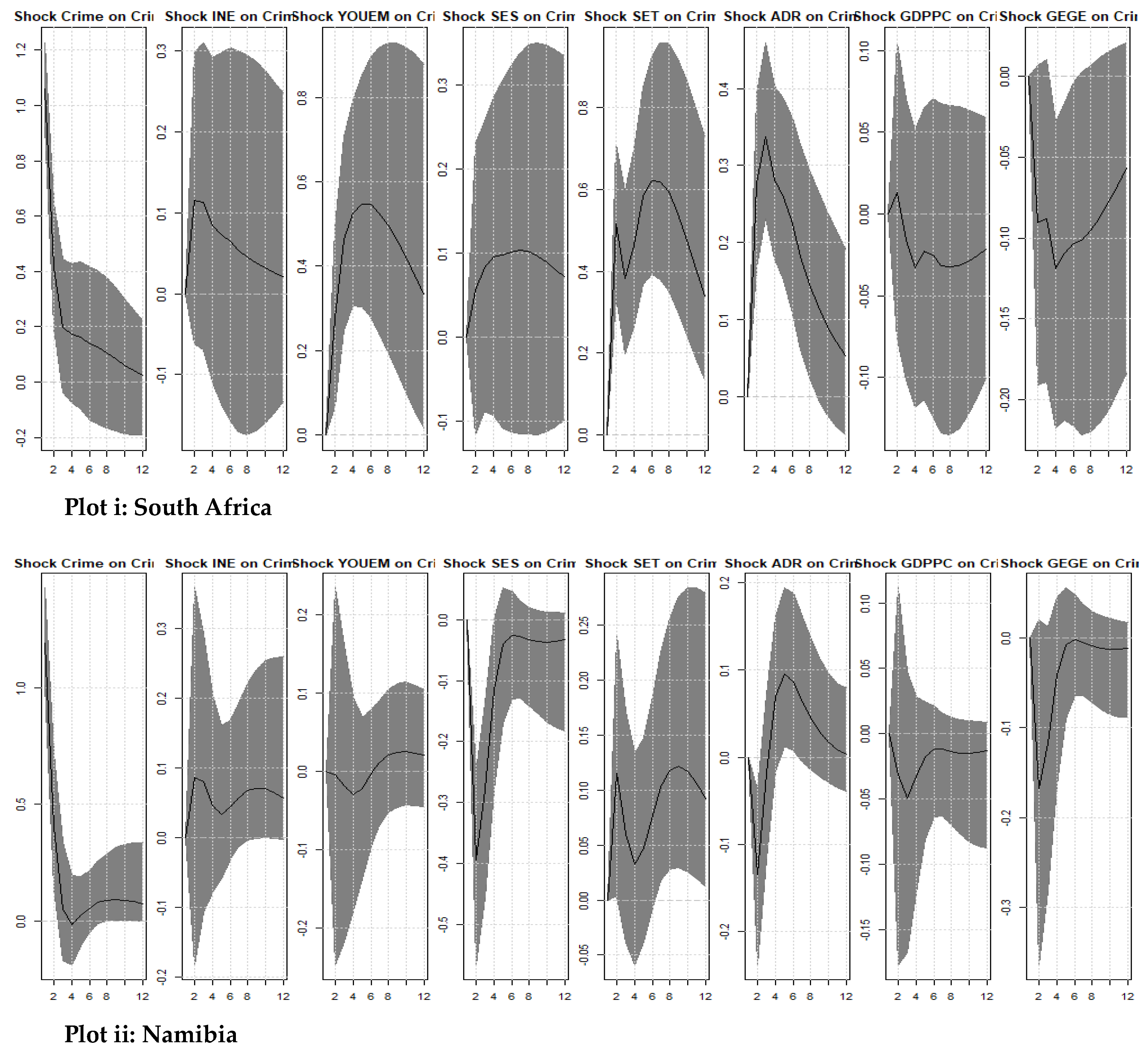
In the South African context, a further rise in crime was recorded as a one percent standard deviation shock to youth unemployment (YOUEM), with a maximum impact of 0.48. This then immediately converged, reverting to the steady-state region and dying after 12 years. The findings are empirical and plausible in the existing literature, such as the study by Raphael and Winter-Ebmer (2001), Lochner (2004), Jenkins and Williams (2009), Mustard (2010), Jacobs and Alpert (2013), Maddah (2013) for Iran; Costantini et al. (2018) for US countries; Khaliq et al. (2019) for Punjab, Pakistan; Lojanica and Obradovic (2019) for Central and Eastern European countries, Mazorodze (2020) for KwaZulu-Natal (KZN), South Africa, and Zungu and Mtshengu (2023) for emerging economies.
In the Namibian context, crime progressively decreased following a one percent standard deviation shock to YOUEM and attaining a maximum impact of 0.05, 4 years after the shock to YOUEM. This then converged immediately, reversing to the steady-state region and dying after 6 years. The results further indicate that the impact of youth unemployment on crime is asymmetrical. While the negative impact of youth unemployment found in Namibia supports the idea postulated by criminologists, who believe that unemployment is adversely related to crime, criminologists also contend that unemployment results in fewer crime victims and stolen goods (Cantor & Land, 1985, 2001; Nunn & O'Donnell, 2019; Di Tella & Schargrodsky, 2020; Chalfin & McCrary, 2021; Lassen & Hougaard, 2021; Owens & Weisburd, 2022)
These articles offer insights into the complex dynamics between unemployment and crime, highlighting situations and factors where the expected positive correlation might not hold or might even reverse. This study highlights the importance of community support systems in reducing crime rates during periods of high unemployment, suggesting that robust community networks and support can lead to a negative or neutral relationship between unemployment and crime.
When we control for School Enrolment, the Secondary (SES) model, we find that the impact of SES on crime is country specific, since we found differing results. For South Africa a positive impact on crime was further recorded following a one percent standard deviation shock to SES, with a maximum impact of 0.1 after six years. This then instantly converged, reverting to the steady-state area but not reaching the dying zone. This might be due to a smaller graph margin. For Namibia, on the other hand, crime progressively dropped, reaching a peak of -0.4 within 2 years after the SES shock, then converging after 2 years, reverting to the steady state area, and dying. The findings are empirical and credible in the current literature on unemployment and crime, such as Crews (2009) for Texas. School enrolment tertiary (SET) was found to promote crime in both South African and Namibian counties. We found that crime responded positively following a one percent standard deviation shock to SET, reaching a peak of 0.55 after 2 years in South Africa and reaching a maximum effect of 0.13 after 4 years. This then promptly converged, reverting back, but above the steady state, as it appeared to have a 0.4 impact after taking form growing above 0.6, which then converged, reverting to the steady state area, and dying after 12 years for South Africa. The findings are empirical and credible in the current literature on unemployment and crime, such as Zungu and Mtshengu (2023) for emerging economies.
Following a one percent standard deviation shock to ADR, crime grows to a maximum effect of 0.35 after 3 years, then converges instantly, reverting to the steady state area and dying after 12 years. In the Namibian case, crime progressively drops and reaches a maximum of 0.15 within two years after the ADR shock, then converges instantly, reverting to the steady state area and dying after 12 years. The impact on Namibia was found to be asymmetric. The findings are empirical and credible in the current literature on unemployment and crime, such as those of Zungu and Mtshengu (2023) for emerging economies. Surprisingly, after a one percent standard deviation GDPPC shock, crime responds positively and achieves a maximum effect of 0.003 within 2 years, then converging after 2 years, reverting to the steady state area and dying. In the instance of South Africa, the impact of GDPPC appears to be asymmetric. We argue that the income inequality incorporated in the model influences the probable rationale behind the favourable impact of per capita income on crime. The findings are empirical and credible in the current literature, such as that of Zungu and Mtshengu (2023) for emerging economies. However, our results were supported in the case of Namibia.
Lastly, crime responds negatively for both countries, following a one percent stan-dard deviation shock to GEGE, and attaining a maximum impact of 0.12 after 4 years, which then converges immediately, reversing to the steady state region and dying after 12 years. For Namibia, it achieves a high of 0.15 and soon converges, reverting to the steady-state region and dying after 6 years. The total influence of fiscal policy on crime via government spending is uneven and durable. The findings are empirical and credible in the current literature, such as the studies by Akpom and Doss (2018), Bethencourt (2022) and Zungu and Mtshengu (2023) for emerging economies.
Figure 2B in plots (ii) and (iv) contains the results of the newly democratised European countries and depicts mixed results for the impact of income inequality and youth unemployment on crime, as it shows that after a one percent standard deviation shock to INE for Lithuania, it appears to be more in creating the risk of crime in Lithuania, reaching a maximum level of 0.02 after 4 years and being statistically not different from zero, which then begins to become more significant after 8 years. The influence does not reach a steady-state zone.
Figure 2.
B: Generated impulse responses of the Bayesian VAR for Europeans newly democratised countries. Source: Author’s calculation based on WDI (2023) and SWIID (Solt, 2020) data.
Figure 2.
B: Generated impulse responses of the Bayesian VAR for Europeans newly democratised countries. Source: Author’s calculation based on WDI (2023) and SWIID (Solt, 2020) data.
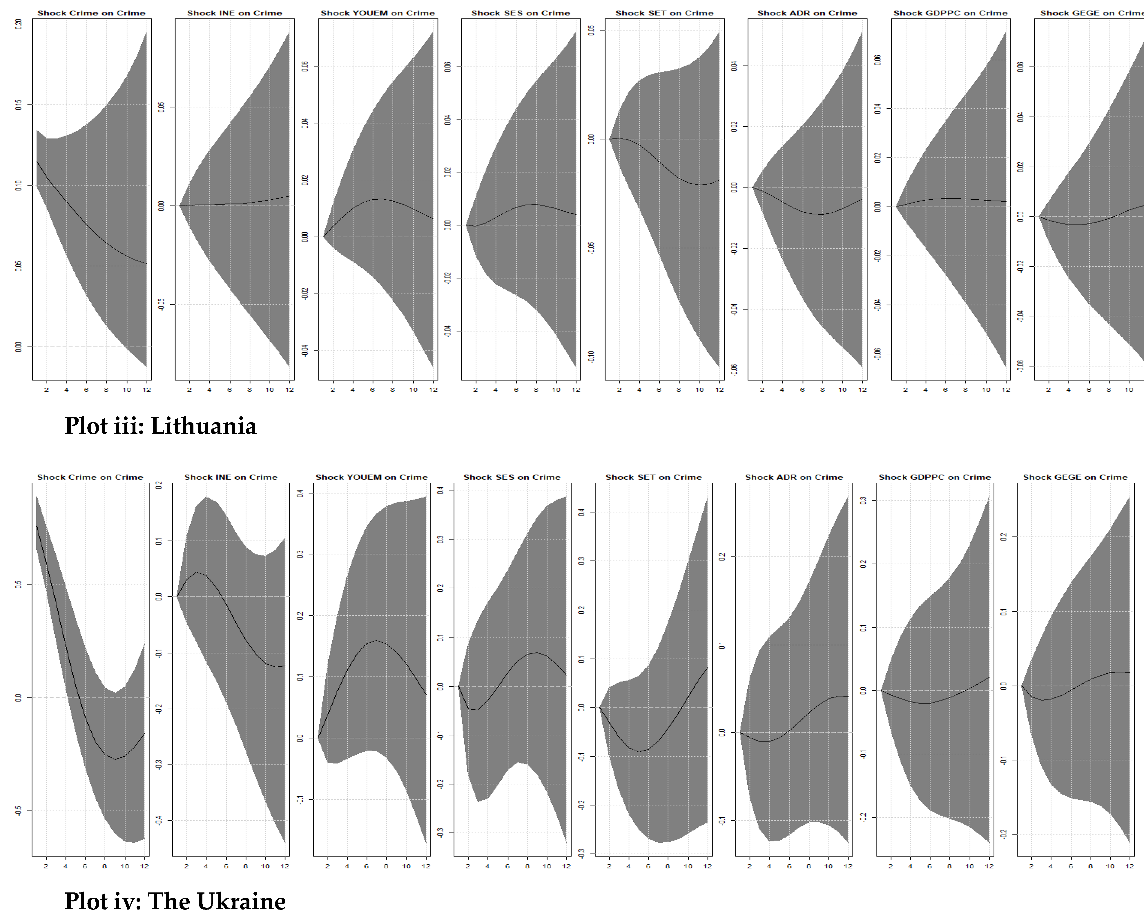
In the case of the Ukraine, the crime responds positively following a one percent standard deviation shock to INE and attains a maximum impact of 0.07 after 4 years, which then converges immediately, reversing to the steady state region and dying after 8 years. The overall impact of income inequality on crime is asymmetric and persistent in the Ukraine. The findings are empirical and credible, such as the current literature on income inequality and crime of Enamorado et al. (2015) for Mexico, Costantini et al. (2018) for US countries, Ngozi and Abdul (2020) for a panel of 38 African countries, Sugiharti et al. (2022) for Indonesia, Jarvenson (2022) for Sweden, and Zungu and Mtshengu (2023) for emerging economies.
Following a one percent standard deviation shock to youth unemployment, both Lithuania and the Ukraine experienced an increase in crime. In the case of Lithuania, the maximum effect is 0.01. After 12 years, this instantly converged, reverting to the steady-state region. For the Ukraine, it attained a maximum impact of 0.18 within 7 years after the YOUEM shock before converging, returning to the steady state region, and dying after 7 years. Our findings are empirical and trustworthy, as they are in line with those studies that reported a positive impact of unemployment and crime, such as those of Maddah (2013) for Iran, Costantini et al. (2018) for US countries, Khaliq et al. (2019) for Punjab, Pakistan, Lojanica and Obradovic (2019) for Central and Eastern European countries, Mazorodze (2020) for KwaZulu-Natal (KZN), South Africa, and Zungu and Mtshengu (2023) for emerging economies.
In the instance of the Ukraine, crime steadily reduced after a one percent standard deviation shock to SES, reaching a maximum impact of -0.08 after 3 years. After 3 years, the impact steadily fades, dying after 12 years. In a nutshell, SES has an asymmetric impact on crime in the Ukraine. In Lithuania, on the other hand, crime responds favourably, peaking at 0.01 within eight years after the shock to SES and then progressively diminishing and dying after seven years. Following a one percent standard deviation shock to SET, crime gradually declines and reaches a minimum level of -0.04, while in the Ukraine it reaches a minimum level of -0.08 in 5 years, then converges, reversing to the steady state region, and dying after 9 years in the Ukraine and 12 years in Lithuania. The findings are empirical and credible in the current literature on unemployment and crime, such as that of Zungu and Mtshengu (2023) for emerging economies. Following a one percent standard deviation shock to ADR, crime steadily declines and reaches a maximum impact of -0.02 after five years. Crime, on the other hand, responds negatively in the Ukraine, reaching a maximum of 0.04 within four years after the ADR shock, and then immediately converging and reverting to the steady state region. In a nutshell, ADR has an asymmetric impact on crime in the Ukraine. The findings are empirical and credible in the current literature on unemployment and crime, such as that of Zungu and Mtshengu (2023) for emerging economies.
Surprisingly, following a one percentage point GDPPC shock, crime responds favourably and achieves a maximum effect of 0.003 after six years, then converges, reverting to the steady-state region, and perishes. Crime in the Ukraine slowly drops and peaks at 0.03 within six years after the GDPPC shock, then converges after 6 years, reverting to the steady state area, and dies. The findings are empirical and credible in the current literature on unemployment and crime, such as that of Zungu and Mtshengu (2023) for emerging economies. Lastly, for both countries, crime responds negatively, following a one percent standard deviation shock to GEGE, and attains a maximum impact of 0.01 after 4 years, which then converges immediately, reversing to the steady state region and dying after 8 years. For Namibia, it achieves a high of 0.05 and soon converges, reverting to the steady-state region and dying after 7 years. The overall impact of a fiscal policy shock to GEGE is asymmetric and persistent. The findings are empirical and credible in the current literature, such as the studies by Akpom and Doss (2018), Bethencourt (2022), and Zungu and Mtshengu (2023) for emerging economies.
Figure 2C in plot v newly democratised Asian countries depict the results of the impact of income inequality (INE) and youth unemployment (YOUEM) on crime in Lithuania due to data unavailability. The results show that crime responds positively following a one percent standard deviation shock to INE in Kyrgyzstan, reaching a maximum level of 0.08 after 2 years, then immediately converges, reverting to the steady state region. The results are in line with the results reported in this study for South Africa, Namibia, Lithuania, and the Ukraine. The overall impact of income inequality on crime is asymmetric and persistent in Kyrgyzstan. The findings are empirical and credible in the current literature on income inequality and crime, such as the studies of Enamorado et al. (2015) for Mexico, Costantini et al. (2018) for US countries, Ngozi and Abdul (2020) for a panel of 38 African countries, Sugiharti et al. (2022) for Indonesia, Jarvenson (2022) for Sweden, and Zungu and Mtshengu (2023) for emerging economies.
Figure 2.
C: Generated impulse responses of the Bayesian VAR for Asian newly democratised countries. Plot v: Kyrgyzstan Source: Author’s calculation based on WDI (2023) and SWIID (Solt, 2020) data.
Figure 2.
C: Generated impulse responses of the Bayesian VAR for Asian newly democratised countries. Plot v: Kyrgyzstan Source: Author’s calculation based on WDI (2023) and SWIID (Solt, 2020) data.
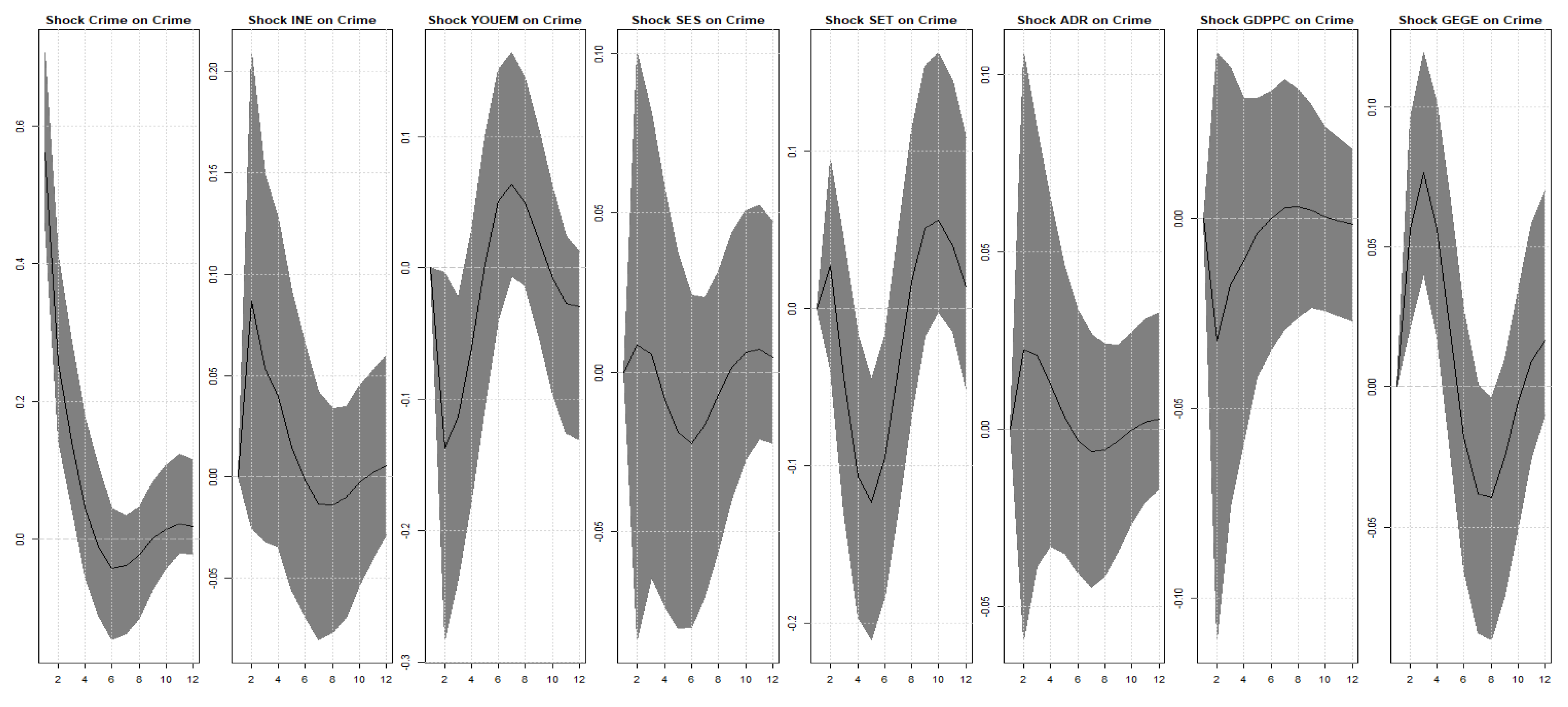
Comparable to what is reported in the case of Namibia, the finding for Kyrgyzstan shows that crime responds negatively following a one percent increase in youth unemployment (YOUEM) and reaches a maximum impact of 0.13 within 2 years before converging, reverting to the steady state region, and dying after 4 years. The overall impact of income inequality on crime is asymmetric and persistent. The findings are empirical and credible in the current literature on unemployment and crime, such as those of criminologists, who believe that unemployment is adversely related to crime. They contend that unemployment results in fewer crime victims and stolen goods (Cantor & Land, 1985, 2001; Nunn & O'Donnell, 2019; Di Tella & Schargrodsky, 2020; Chalfin & McCrary, 2021; Lassen& Hougaard, 2021; Owens & Weisburd, 2022). The logic behind the negative impact of youth unemployment on crime can be explained as follows: Youth unemployment can decrease crime by offering young individuals opportunities for personal and professional growth. When provided with stable jobs, they are less likely to engage in criminal activities due to increased financial security. Employment also creates a sense of responsibility and purpose, diverting their focus away from illicit activities.
Crime responded positively following a one percent standard deviation shock to SES, reaching a maximum impact of 0.02 after two years. After that, it converged to go beyond the steady states, attaining the maximum impact of 0.03; after which it converged again, going back to the steady state region. In a nutshell, SES has an asymmetric impact on crime in Kyrgyzstan. The findings are empirical and credible in the current literature on unemployment and crime, such as that of Zungu and Mtshengu (2023) for emerging economies. The results for Kyrgyzstan further demonstrate that crime responds positively following a one percent standard deviation shock to SET and reaches a maximum impact of 0.02 after 4 years, to go beyond the steady states, attaining a maximum impact of 0.11; after that, it converges again, going back to the steady state region. SET has an asymmetric impact on crime in Kyrgyzstan. The findings are empirical and credible in the current literature on unemployment and crime, such as Zungu and Mtshengu (2023) for emerging economies.
Following a one percent standard deviation shock to ADR, crime steadily increases, reaching a maximum of 0.04 within four years after the ADR shock, and this immediately converges, reverting to the steady state region. In a nutshell, ADR has an asymmetric impact on crime. The findings are empirical and credible in the current literature on unemployment and crime, such as Zungu and Mtshengu (2023) for emerging economies. As expected, following a one percentage point GDPPC shock, crime steadily decreased, attaining a maximum effect of 0.03 after 2 years, then converged, reverting to the steady-state region, and perished. The findings are empirical and credible in the current literature on unemployment and crime, such as Zungu and Mtshengu (2023) for emerging economies.
Lastly, crime responds positively, following a one percent standard deviation shock to fiscal policy (GEGE) and attaining a maximum impact of 0.07 after 3 years, which then converges immediately, reversing and going beyond the steady state region, attaining the maximum impact of 0.04 and dying after 10 years. The overall impact of a fiscal policy shock to financial fragility is asymmetric and persistent. The findings are empirical and credible in the current literature, such as that of Akpom and Doss (2018), and Bethencourt (2022). Government spending can potentially reduce crime by strengthening law enforcement, providing economic and social opportunities, and implementing community policing programs. Increased funding for education and job training can create employment, improve income, and increase social mobility, reducing criminal activity. Mental health programs can address crime's root causes and rehabilitate offenders.
4.3.3. Discussion of the Bayesian VAR Results.
Unemployment and income inequality are two significant factors that have been linked to increased crime rates in societies. High levels of unemployment mean that individuals are often deprived of the opportunity to earn a living wage, which can push them towards illegal or illicit means to survive. Additionally, unemployment can lead to social exclusion, loss of self-worth, and decreased social mobility, which can ultimately result in detrimental mental health outcomes and criminal acts. In addition, income inequality serves as another social factor that can contribute to increased crime rates. When there is a significant gap between the rich and the poor, it results in a concentration of economic power in the hands of a few, while others struggle to merely survive (Fajnzylber, et al., 2002; Wilkinson & Pickett. 2009; Western 2006; Enamorado et al., 2015; Aguirre et al., 2016; Costantini et al., 2018; Stephen & Roeger, 2019; Ngozi & Abdul, 2020; Sugiharti et al., 2022; Jarvenson, 2022; Zungu & Mtshengu, 2023). This leads to feelings of resentment and frustration among those who are disadvantaged, and they may feel compelled to engage in criminal activity as a means of retribution or to gain material goods. Furthermore, income inequality can lead to alienation and a lack of social cohesion, which can result in increased crime rates as individuals turn to illegal behaviour as a means of finding a sense of belonging. In a society where economic disparity is prevalent, it is not uncommon for individuals to resort to drug use, violence, or theft to cope with their feelings of isolation. Therefore, unemployment and income inequality are significant factors that contribute to increased crime rates in societies. Government intervention in the eco-nomy by means of government expenditures then becomes necessary. The findings reveal that government expenditure can decrease crime by strengthening law enforcement agencies, providing economic and social opportunities to citizens, and implementing community policing programs. Increased funding for education and job training programs can create employment, better income, and social mobility, which reduces the likelihood of criminal activity. Moreover, spending on mental health programs can address the root causes of crime and rehabilitate offenders. The results of the robustness check can be found in Appendix A, generated using the fixed-effects model.
4.4. Sensitivity Analysis and Robustness Checks Using the BGMM Models
For the robustness and sensitivity check we used a different approach from the baseline methodology. Unlike the time series: 1) We adopted the panel methodology to further model the impact of these socioeconomic issues in the selected regions. The advantages of the panel data account for the cross-sectional dimension. 2) We used the Palma ratio (inc. Palma) to capture income inequality, while for unemployment, we used the male unemployment rate. 3) As stated in the methodology, we controlled monetary policy variables using house price (HP) as a control variable. Other variables have the same definitions as defined in the baseline methodology. We then adopted a fixed-effects (FE) model to make sure that the results were not sensitive to the model used and to further generate the coefficient impact of these variables on crime. The FE was estimated to support the results of the BVAR. Due to data unavailability for Uzbekistan, we cut our time period to start from 1998–2019. The results of the robustness and sensitivity checks are reported in Table 3.
The results of the FE empirically support the results reported in the baseline me-thodology of this study. We find a positive relationship between income inequality captured by the Palma ratio (incPalma) and crime in models vi, viii, and x. A further positive impact was documented, similar to the results of the baseline model when we used male unemployment to capture the unemployment rate, as it shows in Table 3, Models vii, xi, and xi.
The magnitude of income inequality-crime and unemployment-crime for NDAC is twice that of the coefficient reported in the models in viii, ix, x, and xi for NDEC and NDASC. For the income inequality-crime model iv, the magnitude is 7.80 for NDAC, while in model vii for NDEC, it is 3.10, and for NDASC in x, it is 4.20. while for the unemployment-crime model, the magnitude is 5.97 for the NDAC in vii, for the NDEC in ix, it is 1.67, and for the NDASC in model xi, it is 2.40. These findings signify two things: 1) The results reported in the baseline methodology are not sensitive to the variable used or the model adopted; and 2) the impact of these socioeconomic issues is more severe in African countries than in other regions adopted in the study. We believe these findings hold significant information for policymakers. We then controlled for monetary policy in our model using the house prices. The results show that the house prices emerged with a po-sitive relationship to crime in all models. Our findings support the results documented by Song et al. (2019) for China.
5. Concluding Remarks and Policy Recommendations
This study aims to contribute to the literature by empirically demonstrating the impact of socio-economic issues on crime in newly democratised African countries (South Africa and Namibia) compared to those of recently democratised European countries (Lithuania and the Ukraine) and newly democratised Asian countries (Kyrgyzstan) from 1994 to 2019. The concept of democratisation comes with a number of challenges, depending on how the countries gain their independence. The relationship in this subject matter is complex and multifaceted, particularly in countries with diverse socio-economic landscapes, such as the countries adopted in this study. All these countries, except Ukraine, are similarly characterised by high income inequality accompanied by significant unemployment rates. These socio-economic conditions have historically contributed to high crime rates, particularly violent crimes. Ukraine's transition from a planned to a market economy led to economic disparities and unemployment, resulting in increased crime rates post-Soviet. However, recent reforms focusing on economic stability and corruption have positively impacted crime. Strengthening the rule of law and improving governance have created a transparent, fair economic environment, reducing criminal activities linked to economic desperation and inequality. Moreover, data credibility might be one of the issues in these countries. Therefore, to investigate the impact of socio-economic issues on crime, we adopted the Bayesian VAR approach with hierarchical priors. However, before the execution of the hierarchical priors, we first adopted a number of priors to improve the resilience of our results by addressing two measurable defects: when the data quality is uncertain and when it is frequently short. According to our knowledge, no studies have yet investigated the effect of these socio-economic issues on crime, focusing on African countries that have recently gained their independence, defined as newly democratised countries, and compared their results with those of European countries and Asian newly democratised countries. We believe this study is crucial for these countries, as both the economist and government need to have a clear understanding of the impact of these socio-economic issues on society at large. Which then pushes up the individual's willingness to commit crime, as explained in the theoretical literature. We then seek to compare the results to find out what African countries can learn from other regions if they are doing better in fighting against the severe impact of these socio-economic issues in the community. This would help in finding out: what prevents African newly democratised countries from becoming more involved in these topical issues? Furthermore, understanding that these are one of the objectives of the government, we then extend our definition by cooperating fiscal policy through government expenditure on the system, and tracing the impact of government intervention in the economy. The results show that, except for Namibia, in newly democratised African countries and in newly democratised Asian countries (Kyrgyzstan), the current analysis finds a substantial positive impact of these socio-economic issues (income inequality and youth unemployment) on crime in all regions. However, in Namibia and Kyrgyzstan, the impact of youth unemployment on crime is negative, which is the opposite of what was predicted. The findings illustrate that crime responds positively following unexpected 1% increases in youth unemployment and income inequality. The findings are theoretically plausible and consistent with previous studies on income inequality and crime, such as those of Costantini et al. (2018) for the United States, Ngozi and Abdul (2020) for a panel of 38 African countries, Goh and Law (2021) for Brazil, and Zungu and Mtshengu (2023) for emerging economies. Furthermore, our findings on unemployment and crime support those reported by Costantini et al. (2018) using panel data from the United States, Mazorodze (2020) focusing on southern African provinces, particularly KwaZulu-Natal, Siwach (2018) for New York State, and Zungu and Mtshengu (2023) for emerging economies. We then take the argument documented by Zungu and Mtshengu (2023) further by controlling for government intervention through government spending. The findings show that government intervention through government spending plays an essential role in lowering the devastating impact of crime on society in both regions. This is evident from the data, which show that crime decreases adversely in response to unanticipated 1% increases in government spending. The findings reveal that increasing income inequality and youth unemployment contribute to the growing level of crime in these regions, emphasizing that policymakers should be concerned about excessive inequality and high levels of unemployment, particularly among the youth. To fight against increasing levels of income inequality and unemployment, a comprehensive policy strategy is needed. Key areas of focus include job creation and economic empowerment, which involve developing programs targeting marginalised and high-crime areas, investing in education systems, strengthening social safety nets, implementing equitable income distribution policies, supporting community development and social cohesion initiatives, and designing inclusive economic policies. Job creation programs should focus on creating jobs, particularly in underserved communities, and supporting small and medium-sized enterprises (SMEs) through access to credit, training, and market opportunities. Education systems should ensure quality and accessibility for all, particularly in underserved communities. Strengthening social safety nets, such as unemployment benefits, child support grants, access to housing and food security programs, can reduce economic desperation and the temptation to engage in criminal activities. The intervention of the government through government expenditure programs is also crucial in these economics in fostering equity and reducing the temptations to commit crime. Beyond these results, inclusive economic policies should be designed to ensure economic benefits are widely shared across all segments of society. Regular monitoring and evaluation of these policies can optimize their effectiveness.
Author Contributions
[removed due to the anonymity of peer review process].
Funding
This research received no external funding.
Data Availability Statement
[removed due to the anonymity of peer review process].
Acknowledgments
[removed due to the anonymity of peer review process].
Conflicts of Interest
The author(s) declare(s) no conflict of interest. Additionally, the funders had no role in the design of the study; in the collection, analyses, or interpretation of data; in the writing of the manuscript, or in the decision to publish the results.
Appendix A

Table A1.
a: Descriptive statistics for South Africa.
| Descriptive Statistics | DF[7] | PP[8] | ||||||||||||
| Variables | Mea | Std.d | Min | Max | SKW | KUR | JB-ST | JB-P | Level | 1st | Inte | Level | 1st | Inte |
| Crime | 10.29 | 13.68 | 6.52 | 60.84 | -0.05 | 2.77 | 93.20 | 0.40 | 0.90 | -6.09*** | I(1) | 0.40 | -4.03*** | I(1) |
| INE | 46.48 | 6.58 | 10.30 | 63.00 | -0.67 | 2.89 | 55.11 | 0.30 | 1.21 | -4.22*** | I(1) | 2.00 | -6.56*** | I(1) |
| Top10 | 48.20 | 10.40 | 12.10 | 64.30 | -0.40 | 3.44 | 14.00 | 0.23 | 1.23 | -4.01*** | I(1) | 2.23 | -6.33*** | I(1) |
| YOU | 17.17 | 6.04 | 5.39 | 60.83 | -0.53 | 2.93 | 19.24 | 0.10 | 2.98 | -5.90** | I(1) | -5.00*** | I(0) | |
| MUN | 19.71 | 8.09 | 0.60 | 59.99 | -0.50 | 2.89 | 22.43 | 0.64 | 1.32 | -3.90*** | I(1) | 2.34 | -5.45** | I(1) |
| EDT | 70.23 | 19.98 | 8.20 | 115.95 | -0.10 | 3.19 | 14.92 | 0.36 | 1.80 | -6.30** | I(1) | 2.04 | 4.40** | I(1) |
| EDS | 48.03 | 6.20 | 5.95 | 41.59 | -0.44 | 2.27 | 18.81 | 0.43 | 0.12 | -4.09** | I(1) | 2.12 | I(0) | |
| AGDY | 72.16 | 19.63 | 25.15 | 102.44 | -0.11 | 2.11 | 15.88 | 0.64 | 2.00 | -4.11*** | I(1) | 0.30 | -9.45*** | I(1) |
| LGDP | 7.04 | 1.18 | 4.79 | 9.68 | -0.41 | 2.87 | 78.29 | 0.62 | 1.29 | -5.00*** | I(1) | 1.20 | -6.40*** | I(1) |
Table A1.
b: Descriptive statistics for Namibia.
| Descriptive Statistics | DF | PP | ||||||||||||
| Variables | Mea | Std.d | Min | Max | SKW | KUR | JB-ST | JB-P | Level | 1st | Inte | Level | 1st | Inte |
| Crime | 18.729 | 2.276 | 14.28 | 23.50 | 0.098 | 2.780 | 0.093 | 0.95 | 2.43 | -5.11*** | I(1) | 2.11 | -11.14*** | I(1) |
| ADR | 73.917 | 6.702 | 66.76 | 83.33 | 0.211 | 1.303 | 3.312 | 0.19 | 2.00 | -4.22*** | I(1) | 4.20 | -9.67 *** | I(1) |
| GDPPC | 8.823 | 0.194 | 7.977 | 8.51 | -0.032 | 1.419 | 2.709 | 0.25 | 0.45 | -5.24*** | I(1) | 3.19 | -13.56*** | I(1) |
| GEGE | 7.473 | 1.412 | 5.760 | 10.63 | 0.692 | 2.347 | 2.536 | 0.28 | 0.56 | -3.94** | I(1) | -4.33*** | I(0) | |
| INE | 66.230 | 0.514 | 65.00 | 67.00 | 0.329 | 2.849 | 0.495 | 0.78 | 1.54 | -4.80*** | I(1) | 3.22 | -7.19** | I(1) |
| SES | 64.716 | 6.163 | 54,67 | 71.42 | -0.455 | 1.741 | 2.615 | 0.27 | 1.90 | -4.29** | I(1) | 1.28 | -9.00** | I(1) |
| SET | 12.050 | 6.990 | 5.169 | 26.63 | 0.744 | 2.009 | 3.467 | 0.17 | 1.10 | -5.83** | I(1) | -8.23** | I(0) | |
| YOUEM | 40.963 | 3.055 | 34.02 | 45.01 | -0.709 | 2.836 | 2.836 | 0.33 | 2.09 | -9.13*** | I(1) | 0.30 | -10.13*** | I(1) |
Table A1.
c: Descriptive statistics for the Ukraine.
| Descriptive Statistics | DF | PP | ||||||||||||
| Variables | Mea | Std.d | Min | Max | SKW | KUR | JB-ST | JB-P | Level | 1st | Inte | Level | 1st | Inte |
| Crime | 7.28 | 1.657 | 4.341 | 10.02 | -0.135 | 1.747 | 1.779 | 0.41 | 3.40 | -6.45*** | I(1) | 3.11 | -10.21*** | I(1) |
| ADR | 45.711 | 2.992 | 41.94 | 51.66 | 0.749 | 2.443 | 2.770 | 0.25 | 0.39 | -4.02*** | I(1) | 3.20 | -2.30*** | I(1) |
| GDPPC | 7.579 | 0.236 | 7.183 | 7.86 | -0.571 | 1.753 | 3.097 | 0.21 | 3.11 | -5.32*** | I(1) | 4.19 | -1.23*** | I(1) |
| GEGE | 5.462 | 0.906 | 3.618 | 7.39 | -0.115 | 2.947 | 0.060 | 0.97 | 0.47 | -4.43** | I(1) | -3.33*** | I(0) | |
| INE | 28.142 | 1.279 | 26.10 | 29.90 | 0.018 | 1.407 | 2.748 | 0.25 | 0.43 | -5.40*** | I(1) | 0.22 | -8.20** | I(1) |
| SES | 5.462 | 0.906 | 3.61 | 7.39 | -0.115 | 2.947 | 0.060 | 0.97 | 1.30 | -4.10** | I(1) | 2.23 | 11.34** | I(1) |
| SET | 68.359 | 17.66 | 40.36 | 88.71 | -0.407 | 1.517 | 3.100 | 0.21 | 2.40 | -5.43** | I(1) | 3.17*** | I(0) | |
| YOUEM | 17.493 | 4.37 | 4.026 | 23.57 | -0.971 | 4.629 | 6.965 | 0.03 | 1.99 | -9.34*** | I(1) | 2.00 | -12.11*** | I(1) |
Table A1.
d: Descriptive statistics for Lithuania.
| Descriptive Statistics | DF | PP | ||||||||||||
| Variables | Mea | Std.d | Min | Max | SKW | KUR | JB-ST | JB-P | Level | 1st | Inte | Level | 1st | Inte |
| Crime | 8.404 | 2.574 | 4.533 | 13.84 | 0.15 | 2.22 | 0.75 | 0.68 | 0.30 | -4.54*** | I(1) | 1.14 | -7.21*** | I(1) |
| ADR | 25.844 | 4.184 | 21.85 | 33.51 | 0.64 | 1.84 | 3.27 | 0.19 | 1.59 | -5.22*** | I(1) | 2.54 | -5.30*** | I(1) |
| GDPPC | 8.820 | 0.646 | 7.667 | 9.77 | -0.27 | 1.82 | 1.83 | 0.40 | 0.41 | -3.32*** | I(1) | 2.19 | -9.33*** | I(1) |
| GEGE | 19.864 | 2.966 | 16.29 | 25.88 | 0.51 | 1.94 | 2.36 | 0.30 | 3.07 | -5.94*** | I(1) | -4.43*** | I(0) | |
| INE | 33.45 | 1.769 | 30.50 | 36.20 | 0.12 | 1.94 | 1.27 | 0.52 | 1.32 | -4.54*** | I(1) | 2.32 | -5.34** | I(1) |
| SES | 101.65 | 7.989 | 82.86 | 108.99 | -1.16 | 3.02 | 5.88 | 0.05 | 2.34 | -6.50** | I(1) | 1.48 | 12.54** | I(1) |
| SET | 64.818 | 20.14 | 25.84 | 89.25 | -0.82 | 2.33 | 3.40 | 0.18 | 2.43 | -4.34*** | I(1) | -6.12*** | I(0) | |
| YOUEM | 9.898 | 2.544 | 4.34 | 14.97 | -0.05 | 3.08 | 0.02 | 0.98 | 3.43 | -4.19*** | I(1) | 1.40 | -7.13*** | I(1) |
| Crime | 8.404 | 2.574 | 4.533 | 13.84 | 0.15 | 2.22 | 0.75 | 0.68 | 2.54 | -4.30*** | I(1) | 2.20 | -6.30*** | I(1) |
Table A1.
e: Descriptive statistics for Kyrgyzstan.
| Descriptive Statistics | DF | PP | ||||||||||||
| Variables | Mea | Std.d | Min | Max | SKW | KUR | JB-ST | JB-P | Level | 1st | Inte | Level | 1st | Inte |
| Crime | 7.94 | 3.12 | 2.18 | 16.76 | 0.42 | 4.08 | 2.05 | 0.35 | 0.70 | -6.35*** | I(1) | 1.12 | -7.34*** | I(1) |
| ADR | 25.84 | 4.18 | 21.85 | 33.51 | 0.64 | 1.84 | 3.27 | 0.19 | 2.43 | -3.54*** | I(1) | 2.30 | -6.54*** | I(1) |
| GDPPC | 8.82 | 0.64 | 7.66 | 9.77 | -0.27 | 1.82 | 1.83 | 0.40 | 0.10 | -4.42*** | I(1) | 0.15 | -6.43*** | I(1) |
| GEGE | 45.31 | 11.05 | 22.73 | 61.74 | -0.66 | 2.39 | 2.32 | 0.31 | 2.43 | -7.32** | I(1) | -4.02*** | I(0) | |
| INE | 34.31 | 1.20 | 32.40 | 36.30 | -0.08 | 1.90 | 1.33 | 0.51 | 1.43 | -3.50*** | I(1) | 2.43 | -6.44** | I(1) |
| SES | 13.25 | 1.41 | 10.17 | 15.13 | -0.40 | 2.02 | 1.73 | 0.41 | 0.34 | -4.23** | I(1) | 2.43 | 7.40** | I(1) |
| SET | 100.23 | 7.35 | 90.37 | 114.24 | 0.80 | 2.42 | 3.12 | 0.20 | 2.34 | -6.43** | I(1) | -3.54*** | I(0) | |
| YOUEM | 9.37 | 2.35 | 5.77 | 15.53 | 0.80 | 3.29 | 2.90 | 0.23 | 3.34 | -5.23*** | I(1) | 0.36 | -6.23*** | I(1) |
Table A2.
Lag selection-criteria.
| Lag | CD | J | J-P.v | MBIC | MAIC | MQIC |
| 1 | 0.99 | 173.59 | .30 | −522.20 | −100.10 | −276.13 |
| 2 | 0.99 | 120.20 | .39 | −430.11 | −73.78 | −130.10 |
| 3 | 0.99 | 62.80 | .45 | −334.56 | −56.30 | −104.20 |
| 4 | 0.99 | 19.33 | .53 | −109.20 | −31.19 | −60.21 |
| 5 | 0.99 | 9.45 | .23 | −100.00 | −10.32 | −50.09 |
| 6 | 0.99 | ….. | … | …. | …. | …. |
Source: Author’s illustration based on SWIID (Solt 2020; WDI 2023).
Table A3.
Income Inequality, unemployment, and crime; EF model, newly democratised African and newly democratised European Countries.
Table A3.
Income Inequality, unemployment, and crime; EF model, newly democratised African and newly democratised European Countries.
| Variables | Fixed Effect Model | |||
| Newly democratised African | Newly democratised European | |||
| Model v: Income Inequality | Model vi: Unemployment | Model vii: Income Inequality | Model viii: Unemployment | |
| Pre-tax National Income (TOP10) | 6.80 ** (1.50) | 3.90 ** (0.87) | ||
| Male Unemployment (MUN) | 3.97 *** (0.99) | 2.67 *** (0.98) | ||
| GDP per Capita (GDPPP) | −3.87 ** (1.00) | −2.09 ** (1.00) | −2.88 ** (0.67) | −4.34 ** (1.40) |
| School Enrolment, Secondary (ESE) | 2.45 ** (0.82) | 1.89 ** (0.30) | 0.80 ** (0.04) | 0.92 ** (0.09) |
| School Enrolment, Tertiary (SET) | −3.10 ** (1.09) | −2.45 ** (0.88) | −2.00 ** (0.09) | −1.20 ** (0.20) |
| Age Dependency (ADR) | 3.40 ** (0.90) | 2.99 ** (1.00) | -3.90 ** (0.80) | -2.99 ** (0.90) |
| Population Growth (EDT | 4.83 *** (1.30) | 2.85 *** (0.88) | 2.99 *** (0.04) | 3.89 *** (1.07) |
| Hansen: p-value | 0.784 | 0.593 | 0.665 | 0.6000 |
| 0.608 | 0.593 | 0.688 | 0.599 | |
Note: Dependent variable is the Crime. The numbers in brackets denote the standard errors in brackets obtained by using the cluster-robust and heteroskedasticity-consistent covariance estimator, allowing for error dependency within individual countries. (***), (**) reflect the 1%, 5% levels of significance, respectively. Source: Author’s illustration based on data UNODC (2019) SWIID (Solt 2020; WDI 2023).
For the robustness and sensitivity models, we used the pre-tax national income top 10% from the world inequality database to measure income inequality and the male unemployment rate to capture the unemployment rate. Other variables have the same definition as defined in the baseline methodology. We then adopted a Fixed-effects (FE) model to make sure that the results were not sensitive to the model used. The Fixed- effects Model was estimated in our model to support the result of the PVAR and further generate the coefficient impact of income inequality and unemployment on crime in both regions. The results of the S-GMM and FE empirically support the results reported in the baseline methodology of this study. We find a positive relationship between income inequality captured by the pre-tax national income (TOP10) and crime in model in both regions.
References
- Achim, M.V., Borlea, S.N. & Văidean, V.L.(2021). Does technology matter for combating economic and financial crime? A panel data study. Technological and Economic Development of Economy, 2, 223-261.
- Adeleye, B.N. & Jamal, A. (2020). Dynamic analysis of violent crime and income inequality in Africa. International Journal of Economics, Commerce and Management, 8, 1-25.
- Akpom, U.N & Adrian D. Doss, A.D. (2018). Estimating the impact of state government spending and the economy on crime rates. Journals of Law and Conflict Resolution, 10, 9-18.
- Altavilla, C., Brugnolini, L., Gürkaynak, R.S., Motto, R. & Ragusa, G. (2019). Measuring euro area monetary policy. Journal of Monetary Economics, 108, 162-179.
- Alvaredo, F. 5. Alvaredo, F. & Gasparini, L. (2018). Recent trends in inequality and poverty in developing countries. Handbook of income distribution, 2, 697-805.
- Anser, M.K., Yousaf, Z., Nassani, A.A., Alotaibi, S.M., Kabbani, A. & Zaman, K. (2020). Dynamic linkages between poverty, inequality, crime, and social expenditures in a panel of 16 countries: two-step GMM estimates. Journal of Economic Structures, 9, 1-25.
- Anwar, A., Arshed, N. & Anwar, S. (2017). Socio-economic determinants of crime: An empirical study of Pakistan. International Journal of Economics and Financial Issues, 7, 312-322.
- Ayhan, F. & Bursa, N. (2019). Unemployment and crime nexus in European Union countries: A panel data analysis. Yönetim Bilimleri Dergisi, 17, 465-484.
- Babura, M., Domenico, G., & Lucrezia, R. (2010). Large Bayesian vector auto regressions. Journal of Applied Econometrics, 25, 71–92.
- Becker, G.S. (1968). Crime and punishment: An economic approach. Journal of Political Economy, 76,169-217.
- Bethencourt, C. (2022). Crime and social expenditure: A political economic approach. European Journal of Political Economy, 75, 102183.
- Breiman, L. (2001). Random forests. Machine Learning, 45, 5-32.
- Britt, C.L. (1994). Crime and Unemployment among Youths in the United States, 1958-1990: A Time Series Analysis. American Journal of Economics and Sociology, 53, 99-109.
- Cantor. D, & Kenneth C. L. (1985). Unemployment and crime rates in the post-World War II United States: A theoretical and empirical analysis. American Sociological Review, 317-332.
- Cantor. D. & Kenneth C.L. (2001). Unemployment and crime rate fluctuations: A comment on Greenberg. Journal of Quantitative Criminology, 17, 329-342.
- Carmichael, F., & Ward, R. (2000). Youth unemployment and crime in the English regions and Wales. Applied Economics, 32, 559-571.
- Costantini, M., Meco, I., & Paradiso, A. (2018). Do inequality, unemployment and deterrence affect crime over the long run? Regional Studies, 52, 558-571.
- Crews, G.A. (2009). Description: Education and Crime (2-05). Work: 21st Century Criminology: A Reference Handbook.
- De Mol, C., Giannone, D., & Reichlin, L. (2008). Forecasting using a large number of predictors: Is Bayesian shrinkage a valid alternative to principal components? Journal of Econometrics, 146, 318-328.
- Del-Negro, M., & Schorfheide, F. (2004). Priors from general equilibrium models for VARs.. International Economic Review, 45, 643-673. [CrossRef]
- Demombynes, G., & Özler, B. (2005). Crime and local inequality in South Africa. Journal of Development Economics, 76, 265-292.
- Doan, T. 22. Doan, T., Litterman, R., & Sims, C. (1984). Forecasting and conditional projection using realistic prior distributions. Econometric Reviews.
- Doyle, J.M., Ahmed, E. & Horn, R.N. (1999). The effects of labor markets and income inequality on crime: evidence from panel data. Southern Economic Journal, 65, 717-738.
- Edmark, K. (2005). Unemployment and crime: Is there a connection? Scandinavian Journal of Economics, 107, 353-373.
- Ehrlich, I. (1975). The deterrent effect of capital punishment: a question of life and death. American Economic Review, 65, 397-417.
- Ehrlich, I. (1996). Crime, Punishment, and the Market for Offenses. Journal of Economic Perspectives, 10, 43-67.
- Enamorado, T., López-Calva, L.F., Rodríguez-Castelán, C. & Winkler, H. (2016). Income inequality and violent crime: Evidence from Mexico's drug war. Journal of Development Economics, 120, 128-143.
- Evans, O. & Kelikume, I., 2019. The impact of poverty, unemployment, inequality, corruption and poor governance on Niger Delta militancy, Boko Haram terrorism and Fulani herdsmen attacks in Nigeria. International Journal of Management, Economics and Social Sciences (IJMESS), 8, 58-80.
- Fajnzylber, P., Lederman, D., & Loayza, N. (2002). Inequality and violent crime. The Journal of Law and Economics, 45, 1-39.
- Felson, M., & Cohen, L.E. (1980). Human ecology and crime: A routine activity approach. Human Ecology, 8, 389-406.
- Fougère, D., Kramarz, F., & Pouget, J. (2009). Youth unemployment and crime in France. Journal of the European Economic Association, 7, 909-938.
- Fredj, J., Cheffou, AI, & Bu, R, (2023). "Revisiting the linkages between oil prices and macroeconomy for the euro area: Does energy inflation still matter?" Energy Economics, l, 127.
- Freeman, R.B. (1999). The economics of crime. Handbook of Labor Economics, 3, 3529-3571.
- Giannone, D., Lenza, M., & Primiceri, G.E. (2015). Prior selection for vector autoregressions. Review of Economics and Statistics, 97, 436-451.
- Goh. L. T., & Siong. H. L. (2021). The crime rate and income inequality in Brazil: A nonlinear ARDL approach. International Journal of Economic Policy in Emerging Economies, 15, 1. Available online: https://www.inderscienceonline.com/doi/pdf/10.1504/ IJEPEE.2022.120063 (accessed on 9 January 2023). (accessed on null).
- Grogger, J. (2006). “An economic model of recent trends in violence.” In: A. Blumstein & J. Wallman (Eds.). The crime drop in America (2nd ed.), pp. 266–287). Cambridge: Cambridge University Press.
- Hooghe, M., Vanhoutte, B., Hardyns, W., & Bircan, T. (2011). Unemployment, inequality, poverty and crime: Spatial distribution patterns of criminal acts in Belgium, 2001–06. The British Journal of Criminology, 51, 1-20.
- Kassem, M., Ali, A., & Audi, M., 2019. Unemployment rate, population density and crime rate in Punjab (Pakistan): an empirical analysis. Bulletin of Business and Economics, 8, 92-104.
- Kelly, M. (2000). Inequality and crime. Review of economics and Statistics, 82, 530-539.
- Khaliq, N., Shabbir, M., & Batool, Z. (2019). Exploring the Influence of Unemployment on Criminal Behavior in Punjab, Pakistan. Global Regional Review, 4, 402-409.
- Kilian L., & Lütkepohl H. (2017). Structural Vector Autoregressive Analysis. Cambridge: Themes in Modern Econometrics. Cambridge University Press.
- Koop, G.M. (2013). Forecasting with medium and large Bayesian VARs. Journal of Applied Econometrics, 28, 177-203.
- Kujala, P., Kallio, J., & Niemelä, M. (2019). Income inequality, poverty, and fear of crime in Europe. SAGE Publications, 53, 163–85.
- Kuschnig, N., & Vashold, L. (2019). BVAR: Bayesian vector autoregressions with hierarchical prior selection in R. Journal of Statistical Software, 100, 1-27.
- Kwon, R., & Cabrera, J.F., 2019. Income inequality and mass shootings in the United States. BMC Public Health, 19, 1-8.
- Lee, C., Olasehinde-Williams, G., & Özkan. O. (2023). Geopolitical oil price uncertainty transmission into core inflation: Evidence from two of the biggest global players, Energy Economic, 126, 106983,.
- Litterman, R. B. (1980). A Bayesian procedure for forecasting with vector autoregressions. Working Paper, Massachusetts Institute of Technology, Cambridge, USA.
- Lobonţ, O.R., Nicolescu, A.C., Moldovan, N.C., & Kuloğlu, A. (2017). The effect of socioeconomic factors on crime rates in Romania: a macro-level analysis. Economic Research - Ekonomska istraživanja, 30, 91-111.
- Lojanica, N., & Obradović, S. (2020). Does unemployment lead to criminal activities? Empirical analysis of cee economies. The European Journal of Applied Economics, 17, 104-112.
- Maddah, M. (2013). An empirical analysis of the relationship between unemployment and theft crimes. International Journal of Economics and Financial Issues, 3, 50-53.
- Mazorodze, B.T. (2020). Youth unemployment and murder crimes in KwaZulu-Natal, South Africa. Cogent Economics & Finance, 8, 1799480.
- McCracken, M.W., & Ng, S. (2016). FRED-MD: A monthly database for macroeconomic research. Journal of Business & Economic Statistics, 34, 574-589.
- Merton, R. (1938). Social structure and anomie. American Sociological Review, 3, 672–82.
- Ozcelebi O., & Tokmakcioglu K. (2022). Assessment of the asymmetric impacts of the geopolitical risk on oil market dynamics. Int J Fin Econ. 27, 275–289.
- Schargrodsky, E., & Freira, L., 2021. Inequality and crime in Latin America and the Caribbean: New data for and old question. Undp lac working paper series. Available online: https://www.undp.org/latin-america/publications/inequality-and-crime-latin-america-and-caribbean-new-data-old-question (accessed on 30 May 2023).
- Schleimer, J.P., Pear, V.A., McCort, C.D., Shev, A.B., De Biasi, A., Tomsich, E., Buggs, S., Laqueur, H.S., & Wintemute, G.J., 2022. Unemployment and crime in US cities during the coronavirus pandemic. Journal of Urban Health, 99(1), 82-91.
- Sims, C.A., & Zha, T. (1998). Bayesian methods for dynamic multivariate models. International Economic Review, 949-968.
- Siwach, G. (2018). Unemployment shocks for individuals on the margin: Exploring recidivism effects. Labour Economics, 52, 231-244.
- Solt, F. (2020). Measuring income inequality across countries and over time: The standardized world income inequality database. Social Science Quarterly, 101, 1183-1199.
- Song. Z., Yan,, T.H., & Jiang, T. (2019). Can the rise in housing price lead to crime? An empirical assessment of China. International Journal of Law, Crime and Justice, 59, 2019.
- Sugiharti, L., Esquivias, M.A., Shaari, M.S., Agustin, L., & Rohmawati, H. (2022). Criminality and Income Inequality in Indonesia. Social Sciences, 11, 142.
- Trumbull, WN. (1989). Estimations of the Economic Model of Crime Using Aggregate and Individual Level Data. Southern Economic Journal, 56, 423-439.
- Twambo, J.U.B.E.R.T., & Mbetwa, S. (2017). Correlation between unemployment and high crime rate among the youth: A case study of Kaunda Square Stage One Township (LUSAKA). The International Journal of Multi-Disciplinary Research, 527, 1-15.
- United Nations Office on Drugs Crime UNODC. (2019). Global Study on Homicide. Vienna. Available online: https://www.unodc.org/gsh/ (accessed on 10 February 2023).
- Villani, M. (2009). Steady-state priors for vector autoregressions. Journal of Applied Econometrics, 24, 630-650.
- World Development Indicators WDI. (2023). World Bank. Washington, DC. Available online: http://data.worldbank.org/data-catalog/ world-development-indicators (accessed on 20 February 2023).
- Zaman. K. (2018). Crime-poverty nexus: An intellectual survey. Forensic Res Criminal International Journal, 6, 327–29.
- Zungu, L.T., & Mtshengu, T.R. (2023). The Twin Impacts of Income Inequality and Unemployment on Murder Crime in African Emerging Economies: A Mixed Models Approach. Economies, 11, 58.
Figure 1.
Graphic analysis of the mean Gini-index, youth unemployment, and crime, 1994–2019. Source: Author’s illustration based on data from UNODC (2019) SWIID (Solt, 2020; WDI, 2023).
Figure 1.
Graphic analysis of the mean Gini-index, youth unemployment, and crime, 1994–2019. Source: Author’s illustration based on data from UNODC (2019) SWIID (Solt, 2020; WDI, 2023).
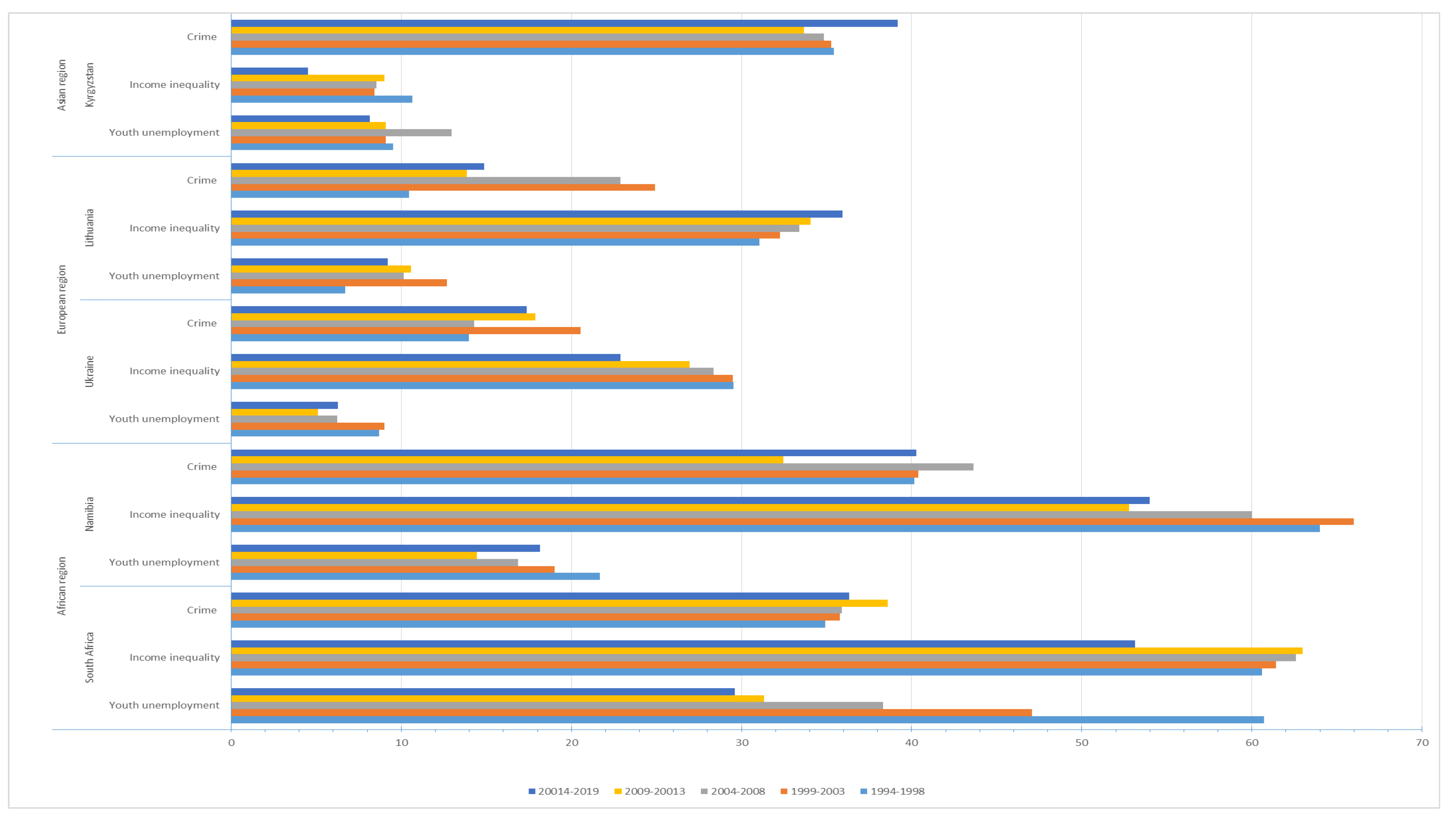
Table 1.
Posterior marginal likelihood.
| NDAC | NDEC | NDASC | ||
|---|---|---|---|---|
| South Africa | Namibia | Lithuania | The Ukraine | Kyrgyzstan |
| Optimisation concluded | ||||
| PMK: -512.20 Hyperparameters: lambda = 1.784 soc = 0.173 sur = 0.547 Finished MCMC after 35.44 minutes |
PMK: -850.99 Hyperparameters: lambda = 1.563 soc = 0.425 sur =0.699 Finished MCMC after 30.45 minutes |
PMK: -677.43 Hyperparameters: lambda = 1.976 soc = 0.320 sur =0.548 Finished MCMC after 35.01 minutes |
PMK: -789.67 Hyperparameters: lambda = 1.994 soc = 0.579 sur =0.354 Finished MCMC after 30.11 minutes |
PMK: -694.04 Hyperparameters: lambda = 1.853 soc = 0.654 sur =0.503 Finished MCMC after 28.58 minutes |
Note: PMK is the posterior marginal likelihood, NDAC, NDEC and NDASC means newly democratised African countries, newly democratised European countries and newly democratised Asian countries, respectively. Source: Author’s calculation based on WDI (2023) and SWIID (Solt, 2020) data.
Table 2.
Summary of the BVAR model.
| NDAC | NDEC | NDASC | ||
|---|---|---|---|---|
| South Africa | Namibia | Lithuania | The Ukraine | Kyrgyzstan |
| BVAR consist of 36 observation, 8 variable and 2 lags. | ||||
| Hyperparameters: lambda, soc, sur HV after optimisation: 1.77, 0.55, 0.60. Iter (burnt / thinn): 1800000 (800000/ 1) Acpt draws (rate): 498356 (0.55). Finished after: 35.44 mins |
Hyperparameters: lambda, soc, sur HV after optimisation: 1.78, 0.21, 0.60. Iter (burnt / thinn): 1800000 (800000/ 1) Acpt draws (rate): 348389 (0.36). Finished after: 30.45 mins |
Hyperparameters: lambda, soc, sur HV after optimisation: 2.88, 0.42, 0.69 Iter (burnt / thinn): 1800000 (800000/ 1) Acpt draws (rate): 443002 (0.35). Finished after: 35.01 mins |
Hyperparameters: lambda, soc, sur HV after optimisation: 1.22, 0.38, 0.50. Iter (burnt / thinn): 1800000 (800000/1) Acpt draws (rate):487706 (0.29). Finished after: 30.11 mins |
Hyperparameters: lambda, soc, sur HV after optimisation: 2.15, 0.43, 0.65. Iter (burnt / thinn): 1800000 (800000/1) Acpt draws (rate):413242 (0.40). Finished after: 28.58 mins |
Note HV means hyperparameter values, and iter refers to iterations, while Acpt means accepted. Source: Author’s calculation based on WDI (2023) and SWIID (Solt, 2020) data.
Table 3.
Income inequality, unemployment, and crime: FE model.
| Variables | NDAC[4] | NDEC[5] | NDASC[6] | |||
|---|---|---|---|---|---|---|
| vi | vii | Viii | ix | x | xi | |
| Palma ratio (incPalma) | 7.80**(1.50) | 3.10**(0.87) | 4.24**(0.43) | |||
| Male unemployment (MUN) | 5.97**(0.99) | 1.67**(0.98) | 2.40**(1.08) | |||
| GDP per capita (GDPPP) | −3.87**(1.00) | −2.09**(1.00) | −2.88**(0.67) | −1.34**(1.40) | -2.54**(0.23) | −2.32**(0.20) |
| School enrolment, Secondary (SES) | 2.45**(0.82) | 1.89** (0.30) | 0.80** (0.04) | 0.92** (0.09) | 0.87**(0.24) | 1.88**(0.29) |
| School enrolment, Tertiary (SET) | −3.10**(1.09) | −2.45**(0.88) | −2.00**(0.09) | −1.20**(0.20) | −2.50**(1.00) | 3.00** (0.50) |
| Age dependency (ADR) | 3.40**(0.90) | 2.99** (1.00) | 3.90** (0.80) | -2.99** (0.90) | 1.81**(0.20) | 3.84**(1.00) |
| Population growth (EDT) | 4.83***(1.30) | 2.85** (0.88) | 2.99* (0.04) | 3.89***(1.07) | 2.18** (0.24) | 2.30** (.30) |
| House price (HP) | 2.03**(0.89) | 1.00**(0.20) | 0.99*(0.44) | 2.40***(0.10) | 3.50**(1.00) | 1.87**(0.59) |
| Hansen: p-value | 0.784 | 0.593 | 0.665 | 0.6000 | 0.5393 | 0.6500 |
| 0.608 | 0.593 | 0.688 | 0.599 | 0.644 | 0.602 | |
Note: The dependent variable is Crime. The numbers in brackets denote the standard errors in brackets obtained by using the cluster-robust and heteroskedasticity-consistent covariance estimator, allowing for error dependency within individual countries. (***), (**) reflect the 1% and 5% levels of significance, respectively. Source: Author’s illustration based on data from the UNODC (2019) and SWIID (Solt 2020; WDI 2023).
| 1 | South Africa and Namibia. |
| 2 | The Ukraine and Lithuania. |
| 3 | Kyrgyzstan. |
| 4 | South Africa and Namibia. |
| 5 | Ukraine and Lithuania. |
| 6 | Kyrgyzstan and Uzbekistan. |
| 7 | Augmented Dickey-Fuller test. |
| 8 | Phillips-Perron test . |
Disclaimer/Publisher’s Note: The statements, opinions and data contained in all publications are solely those of the individual author(s) and contributor(s) and not of MDPI and/or the editor(s). MDPI and/or the editor(s) disclaim responsibility for any injury to people or property resulting from any ideas, methods, instructions or products referred to in the content. |
© 2024 by the authors. Licensee MDPI, Basel, Switzerland. This article is an open access article distributed under the terms and conditions of the Creative Commons Attribution (CC BY) license (http://creativecommons.org/licenses/by/4.0/).
Copyright: This open access article is published under a Creative Commons CC BY 4.0 license, which permit the free download, distribution, and reuse, provided that the author and preprint are cited in any reuse.


