Topological Reinforcement Adaptive Algorithm (TOREADA) Application to Alerting of Convulsive Seizures and Validation with Monte-Carlo Numerical Simulations

Preprint

Article

Topological Reinforcement Adaptive Algorithm (TOREADA) Application to Alerting of Convulsive Seizures and Validation with Monte-Carlo Numerical Simulations

This version is not peer-reviewed.

Stiliyan Kalitzin^*

This version is not peer-reviewed.

Altmetrics

Downloads

Views

Comments

Submitted:

15 October 2024

Posted:

16 October 2024

You are already at the latest version

A peer-reviewed article of this preprint also exists.

Abstract

Detection of adverse events, for example convulsive epileptic seizures, can be critical for the patients suffering from variety of pathological syndromes. Algorithms using remote sensing modalities, such as video camera input, can be effective for real-time alerting but the broad variability of environments and numerous non-stationary factors may limit their precision. In this work, we address the issue of adaptive reinforcement that can provide flexible application of the alerting devices. The generic concept of our approach is the topological reinforced adaptive algorithm (TOREADA. Three essential steps, embedding, assessment and envelope act iteratively during the operation of the system, providing thus a continuous, on the fly reinforced learning. We apply this concept on the case of detecting convulsive epileptic seizures where three parameters define the decision manifold. Monte-Carlo type simulations validate the effectiveness and robustness of the approach. We show that the adaptive procedure finds the correct detection parameters, providing optimal accuracy, from a large variety of initial states. With respect to the separation quality between simulated seizure and normal epochs, the detection reinforcement algorithm is robust within broad margins of signal generation scenarios. We conclude that our technique is applicable to a large variety of event-detection systems.

Keywords:

Subject:

Computer Science and Mathematics - Artificial Intelligence and Machine Learning

1. Introduction

Motor disorders, epileptic seizures with convulsive patterns for example, can have debilitating impact on the lives of affected patients. In cases where therapy has failed, constant safeguarding may be necessary to prevent major complications, injuries or even death as result of sudden attacks or seizures [1,2]. This requires round the clock monitoring in both dedicated facilities and home situation. Although remote video monitoring is now ready available and incorporated in many care systems, it poses certain challenges when operated by human observers. It is extremely labor intensive, operators have to pay uninterrupted attention to multiple screens. In addition, privacy issues may prevent the use of this modality in a variety of cases. Alternative solutions based on attachable devices are also available on the market [3,4] but they also require frequent attention and control for charging, proper positioning etc. Certain patients due to stigmatizing effect of wearing them can also reject the attachable devices.

All the above arguments have motivated us to develop an automated video input based alerting system that is capable of detecting a variety of adverse events such as convulsive motor seizures, falls and non-obstructive apnea [5,6]. Such an approach combines the advantages of remote non-obstructive monitoring, holistic representation of the patient state and automated privacy respecting alerting.

A central issue for such a development is the wide variety of clinical conditions, camera parameters and other environmental factors that can challenge the universality of the algorithms used to provide real-time alerting. To address these challenges we developed adaptive reinforcement concept that can account for non-stationary applications and optimize the detection process accordingly.

In an earlier work, we have addressed the problem of reducing false positive detections by restricting the detection to only validated true positive events [7]. This however, left open the question of missing events, or false negatives. Here we propose a solution that can also expand the detection space and gradually reduce the chance of undetected true events.

To verify the effectiveness of our algorithms, we use synthetic data that can account to a variety of dynamic situations and non-stationary environments.

The paper is organized as follows. In the Methods, we first describe the generic concept of TOREADA (Topological Reinforcement Adaptive Algorithm). Then we present the particular application to convulsive seizure alerting. We introduce the concept of Dual Detection that allows for accounting of missed true seizures and expanding the detection parameters.

We give also a brief introduction to MC (Monte Carlo) type of simulating input data for our classifier and adaptive algorithms.

In the Results section, we present an array of trials demonstrating the effectiveness of our approach for cases of different initial detector states and different levels of separation between events and background signal controlled by the signal generation parameters.

We summarized our major findings in the Conclusions section.

Finally, in the Discussion we state the main motivations for our concept and the assumptions behind. We also acknowledge certain limitations of the approach and propose some directions for further extensions.

2. Materials and Methods

2.1. General Concept of TOREADA

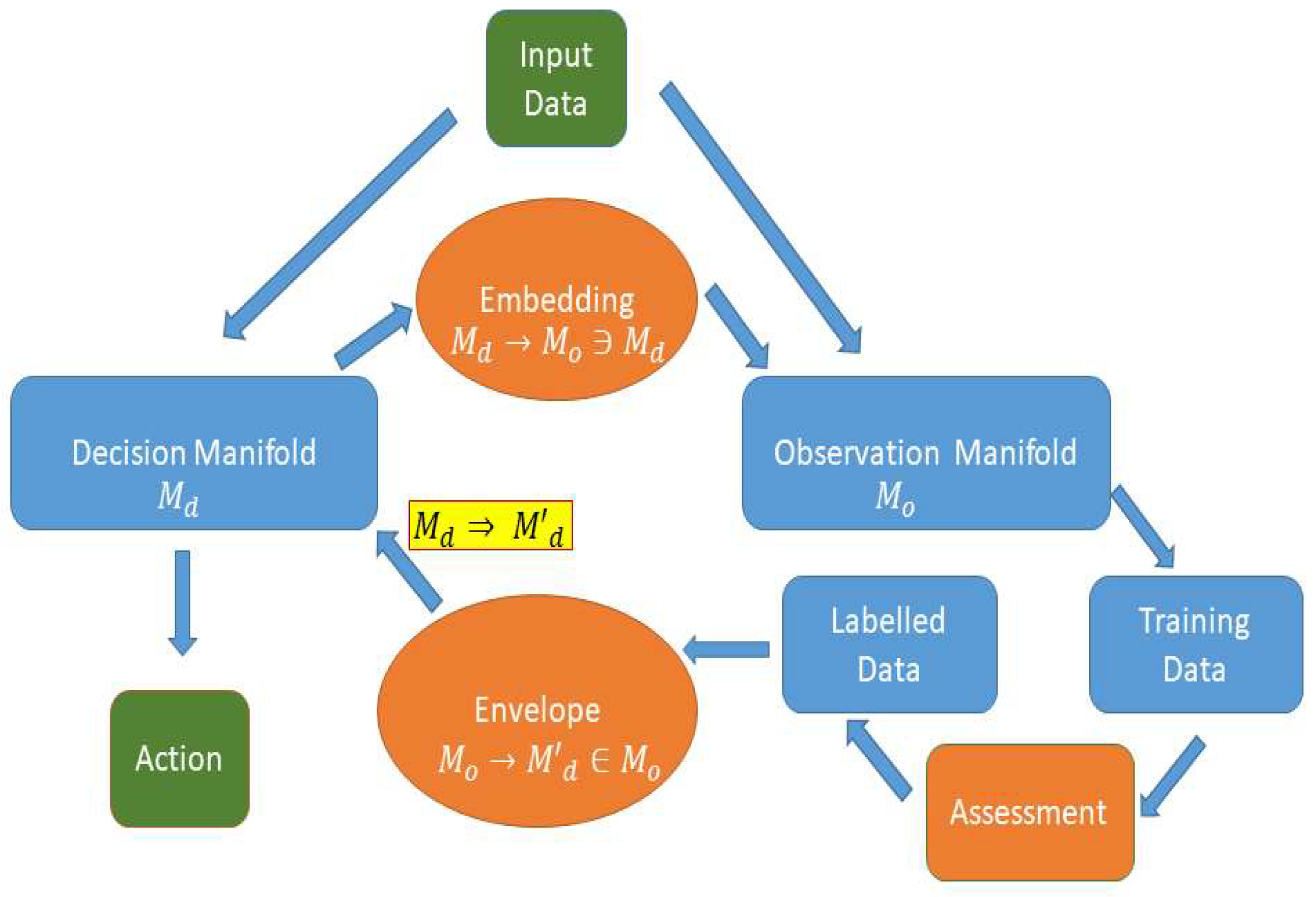
Our approach is of type reinforcement learning that uses constant assessment of the detector performance and accordingly optimizes the parameters. For a general overview and full description of this type of machine learning, we refer to few of the numerous publications available [7,8,9] and here we describe our specific methodology. We illustrate the overall process for the proposed adaptive classification of events on Figure 1.

The generic description of our approach is illustrated on Figure 1. We assume that our system detects certain class of events from an input stream of data. Upon a detection, the system will proceed with a pre-defined action, like raising an alert or simply logging the event. The detection algorithm is encapsulated as

M_{d}

, the “Detection Manifold”. The later can be explicit or implicit (like in case of trained classifiers) but in all cases, we assume that the event features fall into certain area, or manifold that defines them. The adaptive reinforcement involves on-the-move deforming or adapting

M_{d}

according to the performance of the detector. This process must account for both decreasing the number of false detections and for avoiding undetected events. As our training process resorts on only events that are detected and not on screening the whole data history, we introduce an embedding procedure

M_{d} \to M_{o} ∋ M_{d}

(1)

That expands the decision manifold into a larger manifold that may include events missed by the initial detection. These extra events will form a dynamic training set for the adaptive detector but do not affect the output directly (for example no alert will be generated or will be logged separately).

The assessment of the whole set of events is outside the scope of this work. In an earlier work [Kalitzin, Sensors] we proposed a clustering-based algorithm for separating the true from the false events. Alternatively, a trained operator can do the assessment. Here we assume that a labelled set of events is available for the next phase of the training process, the forming of the envelope manifold:

{M_{o} \to M'}_{d} \in M_{o}

(2)

Finally, the reinforcement cycle closes with substituting the initial detection manifold with the envelope from (2):

M_{d} \Rightarrow {M'}_{d}

(3)

The above procedure repeats with every new event or in blocks of pre-defined number of events. It is a learning during the operation scheme that does not require pre-collected data sets.

Equations (1-3) are very abstract and do not reveal any specific algorithm of performing the process. In the next two sub-sections, we provide the specific application to the task of alerting for convulsive epileptic seizures.

2.2. Detection of Convulsive Seizures

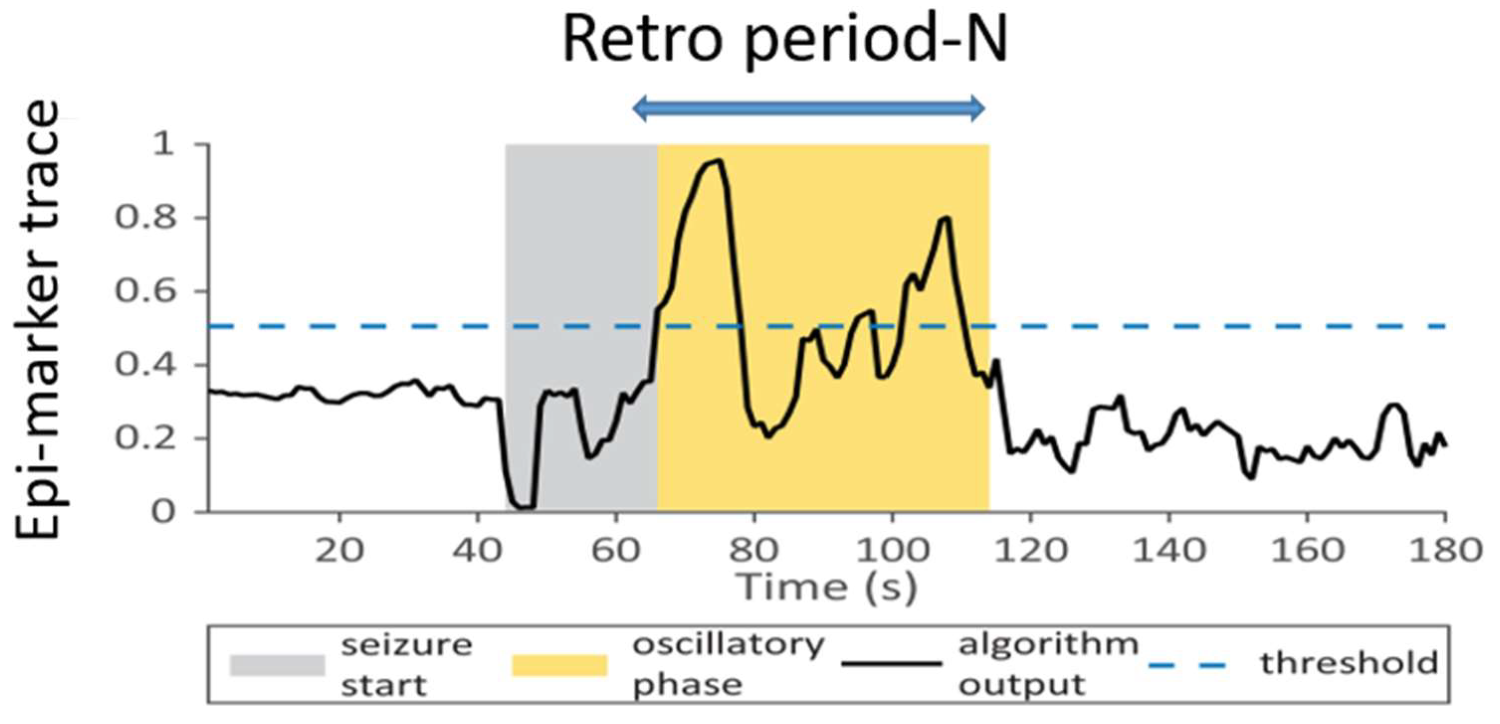
For complete description of seizure detection algorithm, we refer to previous works [11,12]. Here we note that optical flow technique (group-parameter reconstruction) introduced in [13] processes live feed from optical camera and subsequently a set of Gabor filters define a single time series signal that represent the “epileptic content” in the video sequence. Our focus here is only on the last stage of the detection techniques, the decision over whether in a given time-window a convulsive seizure has taken place. We illustrate the decision algorithm on Figure 2.

The following condition defines the decision to define an event of seizure type at any time :

# {s | (s \leq N) & (E (t - s) > T)} \geq n

(4)

Here

E

is the epileptic marker as an input signal,

T

is the selected threshold,

N

is the retrospective time interval (seconds or sample points) and

n \leq N

is the selected minimal amount of time (or number of samples) when the epileptic marker is above the threshold. Note that in (4) we allow for the marker to go up and down across the threshold during the observation period as long as the total time above is longer than

n

According to (4), the three parameters

\{T, N, n\}

define seizure event. It is clear that the higher the threshold the more conservative will be the detection. Also, the longer the interval

N

for a given

n

, the more “liberal” is the detection; more event will fulfil the condition (4). Larger

n

for a fixed

N

defines a stronger condition for an event to be detected as a seizure. Finally, we introduce a “black-out” period

T_{B}

in order to avoid multiple detections of the same event. After a detection, the algorithm skips the next

T_{B}

samples. In all our detections, we have selected a blackout period of 90 samples.

In the next sub-section where we present the embedding and the envelope implementation for this case.

2.3. Dual Detection Approach

The enlargement, or embedding, of the decision space formed by the parameters

\{T, N, n\}

entering inequality (4) postulates the following substitution:

\{T, N, n\} \to \{α T, N + 1, n\} \cup \{α T, N - 1, n - 1\}

(5)

In the transition (5), the union means that if either of the triple fulfils (4), the event is considered as a training event. The parameter

α

is the relative threshold decrease, a reasonable choice is

α = 0.9 .

The embedding (5) is by no means unique but it provides a minimal extension of the decision manifold, close to the detection one. Larger embedding may speed up the inclusion process but may also introduce too many training events that will make the validation phase challenging.

To complete the enforcement procedure, we also need the envelope-forming algorithm. Our earlier work [1] introduced this stage. Here we recall that after the assessment of the training events, we introduced the cost function:

(T, N) = T (2 n (T, N) - N) n (T, N) \equiv {m i n}_{S | T, N} (n)

(6)

In the second equation, the value of the parameter

n

, the filling number, is derived for each pair of

(T, N)

values as the minimal number of threshold-exceeding epochs n over all detected and validated seizure events. This way we can guarantee that, for any choice of the pair

(T, N)

, all the previously detected true seizure events will be preserved. Therefore, we can postulate the optimized choice of parameters as:

\{T, N, n\} : \{T, N\} = a r g m a x (C (T, N); n = n (T, N)

(7)

2.4. Generating Synthetic Data

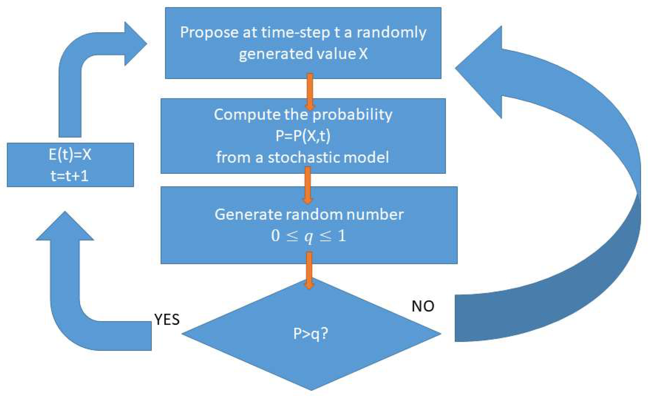
Commonly referred as Monte-Carlo simulation, the synthetic data-generating algorithm consists of a random process driven by a known probability distribution over the states of the system [14]. Figure 3 introduces our implementation that generates a synthetic epileptic marker according to probabilistic rules with pre-defined but variable parameters.

The stochastic model defines the following probabilities for the epi-marker during seizures and outside seizure periods:

P \{E > T_{s}| s e i z u r e\} = P_{s} P \{E > T_{n}| n o r m a l\} = P_{n}

(8)

In equations (8)

T_{s, n}

are the thresholds for correspondingly the ictal and normal periods and

P_{s, n}

are the associated probabilities. We also postulate random ictal onset times. The seizure duration is a a random number in the interval

[L / 2, L]

where

L

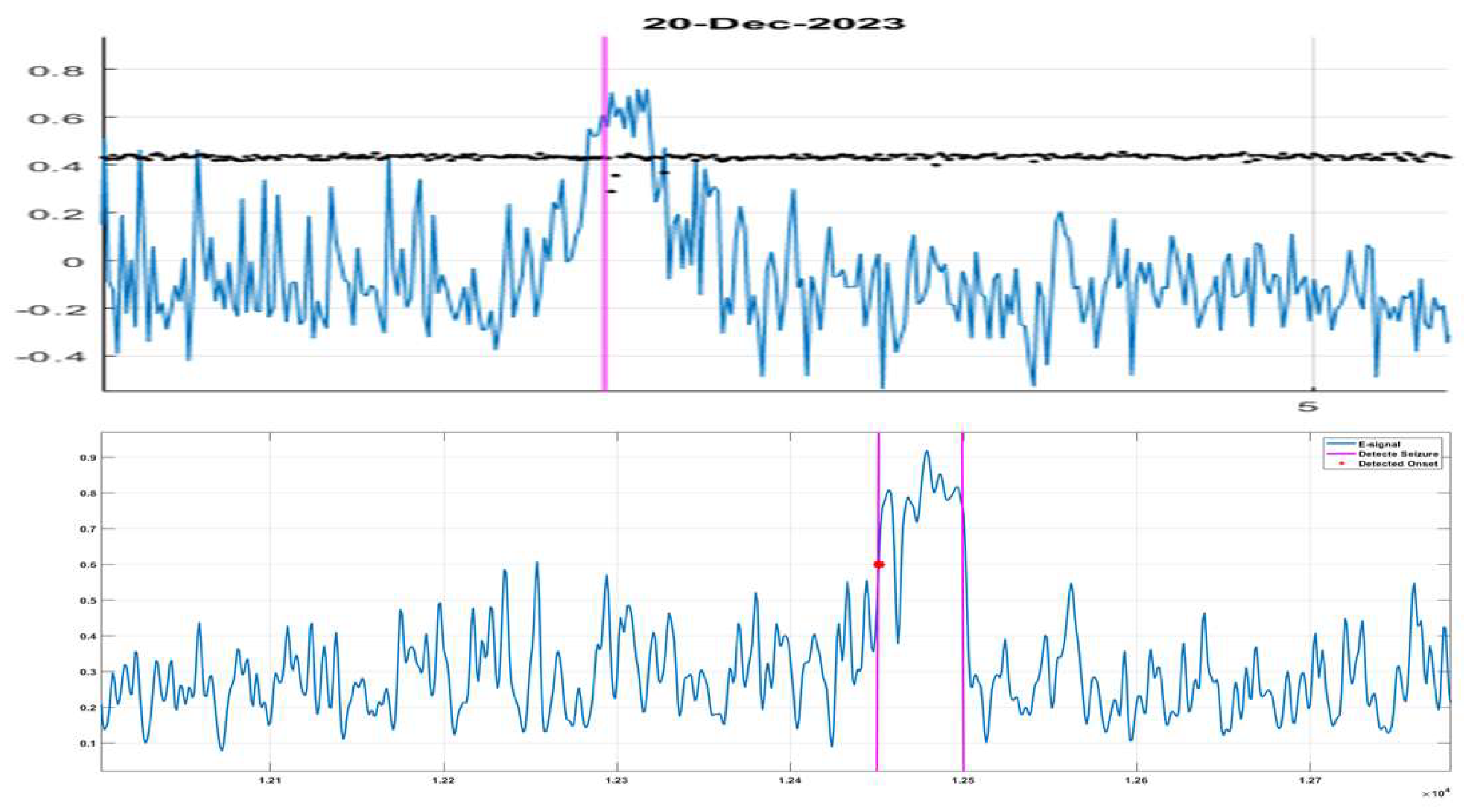
is a chosen maximal duration. We use the generated events as ground truth in order to assess the performance of the detection and reinforcement processes. Figure 4 illustrates a trace of the Epi-marker from a real seizure as observed by our seizure-detection algorithm (top frame) and from a generated event (bottom frame). The parameters for the later are

{T_{s}

T_{n}

P_{s}, P_{n}, L} = {0.8, 0.1, 0.96, 0.05, 30}

In the results below, we consider a variety of scenarios with both stationary and non-stationary seizure generation parameters

{T_{s}

T_{n}

P_{s}, P_{n}

, L}.

To quantify the separation between normal and seizure states, one can use the “confusion” metric between two distributions

p_{n}, p_{s}

defined over the states of any system:

C (p_{n}, p_{s}) \equiv \sum_{s t a t e s} m i n (p_{n}, p_{s})

(9)

Assuming in our case that

T_{s} \geq T_{n}

we obtain from equation (9)

C = T_{n} * \min (1 - P_{n}, 1 - P_{s}) + (T_{s} - T_{n}) * \min (P_{n}, 1 - P_{s}) + (1 - T_{s}) * \min (P_{n}, P_{s})

(10)

2.5. Simulation Protocol and Performance Quantification

We simulate different seizure generating scenarios and initial detection parameters

\{T, N, n\}

Unless otherwise stated, the typical stimulation session includes a number of epochs, each of length 3600 simulation steps. In each epoch, we randomly generate five seizure events according to the stochastic rules explained in the previous sub-section. After each epoch we detect the seizures with the current detector parameters according to sub-section 2.2. . Based on the data generation log, we selected only the true positive events to enter the parameter optimization algorithm. Next, we require a minimum number of 20 retrospectively detected true events in order to start performing the Dual Detection parameter optimization procedure explained in sun-section 2.3. If the number of events is lower than 20, we keep the current parameters. We perform the update after each new simulation epoch, considering no more than 60 previously detected true events in order to account for non-stationary conditions.

After each epoch, we evaluate the detector performance, collecting the statistics from the last 8 epochs (40 generated true events) according to the following standard definitions for the sensitivity and specificity:

S e n s \equiv \frac{T P}{(T P + F N)} S p e c \equiv \frac{T P}{(T P + F P)}

(11)

In equation (11),

T P, F P, F N

are correspondingly the true positive, false positive and false negative (undetected events) detections. The ground truth for the events is according to the simulation log.

3. Results

3.1. Static Seizure Generation Scenarios and Various Initial Detector Parameters

In this set of simulations and detection scenarios, the seizure generation parameters

{T_{s}

T_{n}

P_{s}, P_{n}

, L}={0.4, 0.6, 0.1, 0.96, 0.064, 60} are constant. We only change the initial detector parameters

\{T, N, n\}

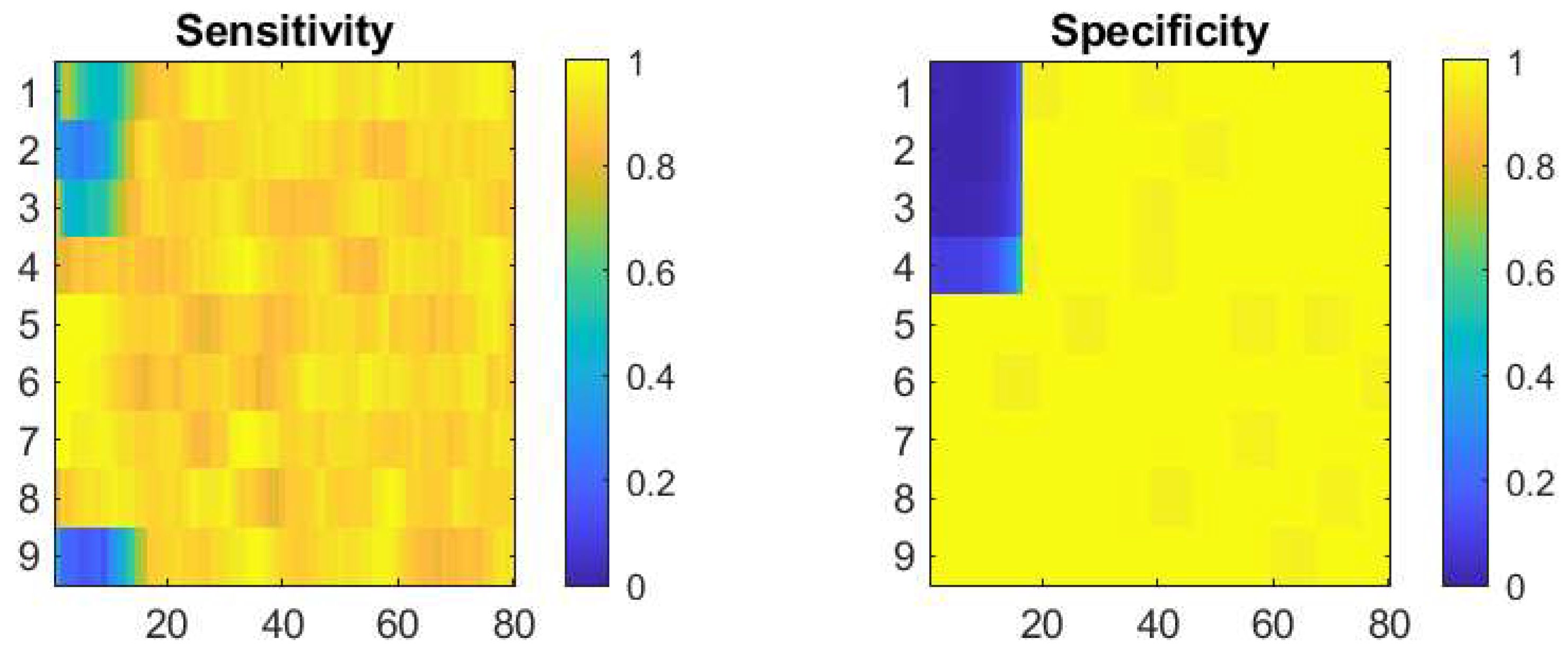
as given in Table 1and register their evolution during the reinforcement process. We present the results on the sensitivity and specificity recovery on Figure 5.

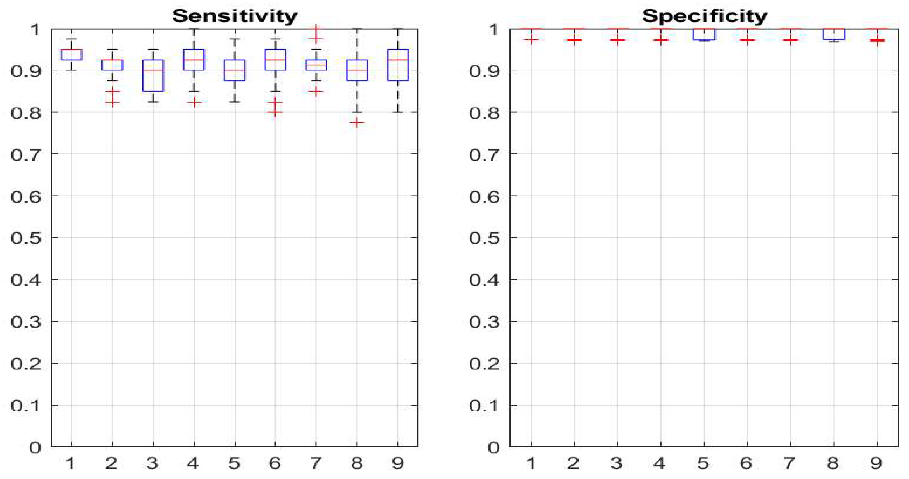
To show the asymptotic behaviour and stability of the reinforcement dynamics, we also present on Figure 6 the boxplots from the distributions of the sensitivity and specificity values taken from the last 50 epochs.

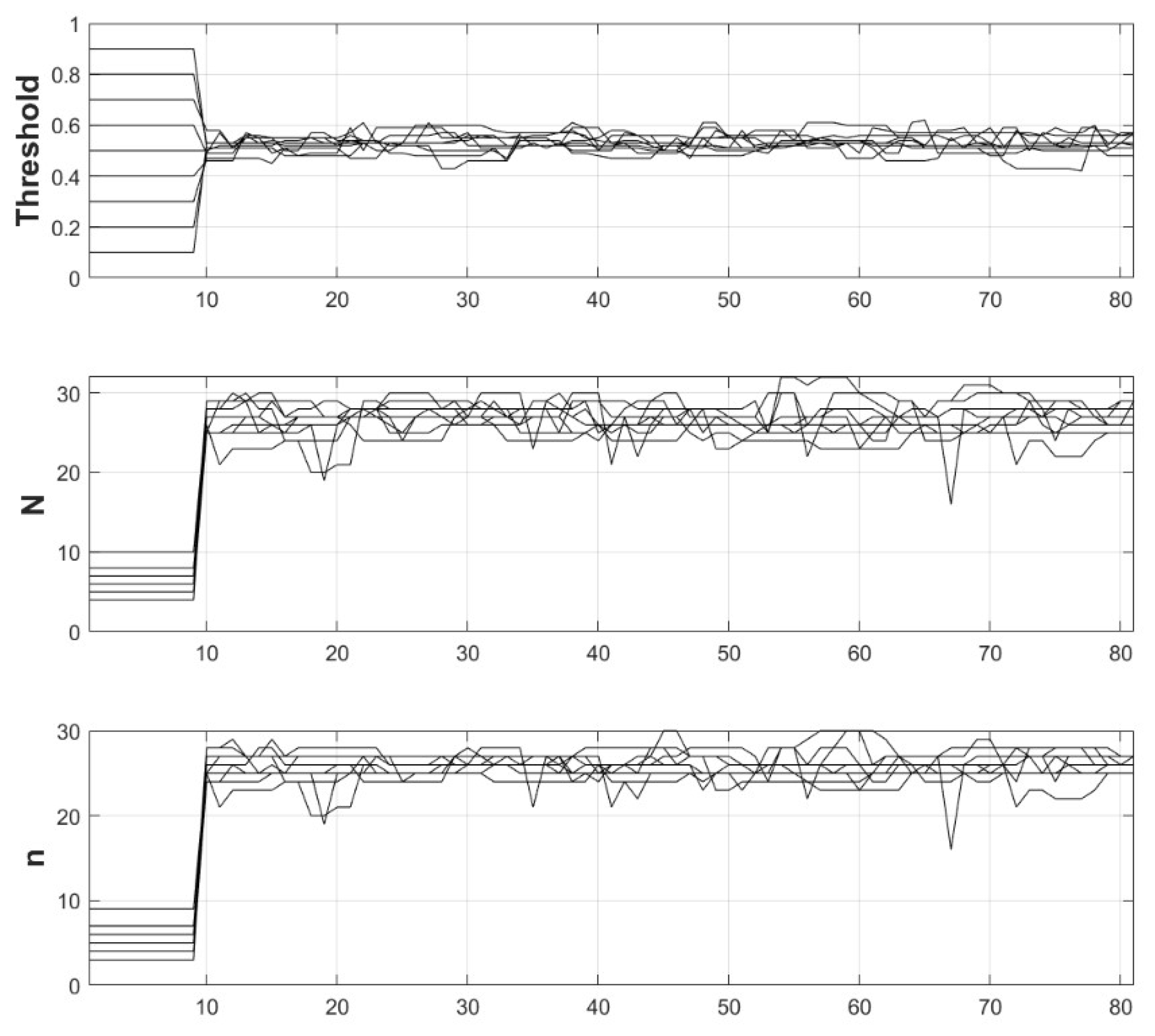
On Figure 7 we show the evolution of the detection parameters.

3.2. Change of Seizure Generation Parameters

Here we perform two simulation experiments aimed at testing the limits of the proposed reinforcement paradigm. Both consist of three separate tests, starting with three different sets of initial detector parameters shown in Table 2.

In the first experiment, we generate seizures with the same maximal duration (60 samples) but with a variety of parameters

T_{s}

T_{n}

P_{s}, P_{n}

presented in Table 3.

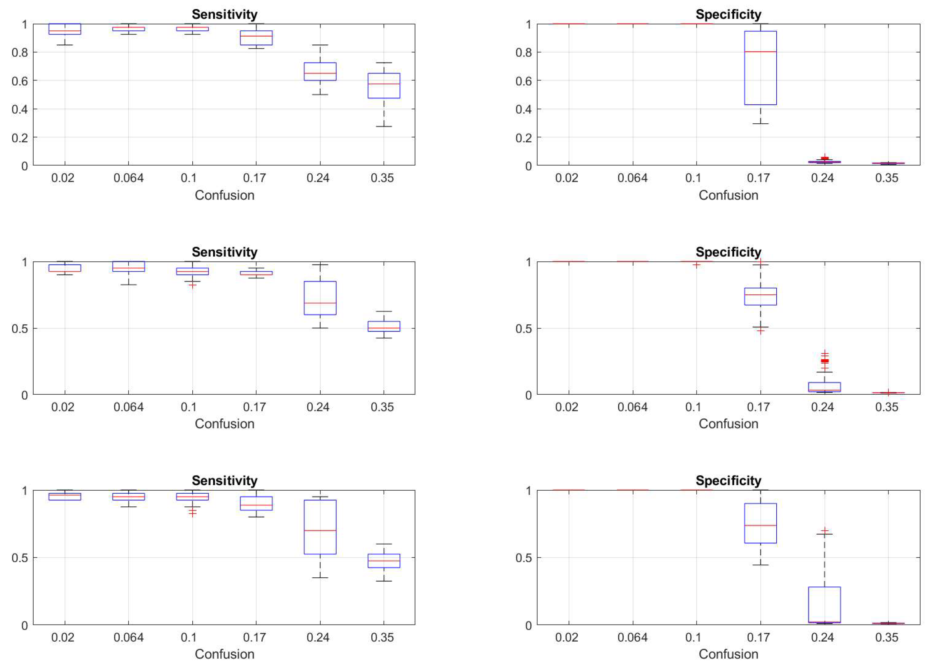
On Figure 8, we show the results of this reinforcement simulation experiment.

Figure 9 represents the statistics of the asymptotic behavior of the reinforcement procedure for these tests, taking again the last 50 epochs.

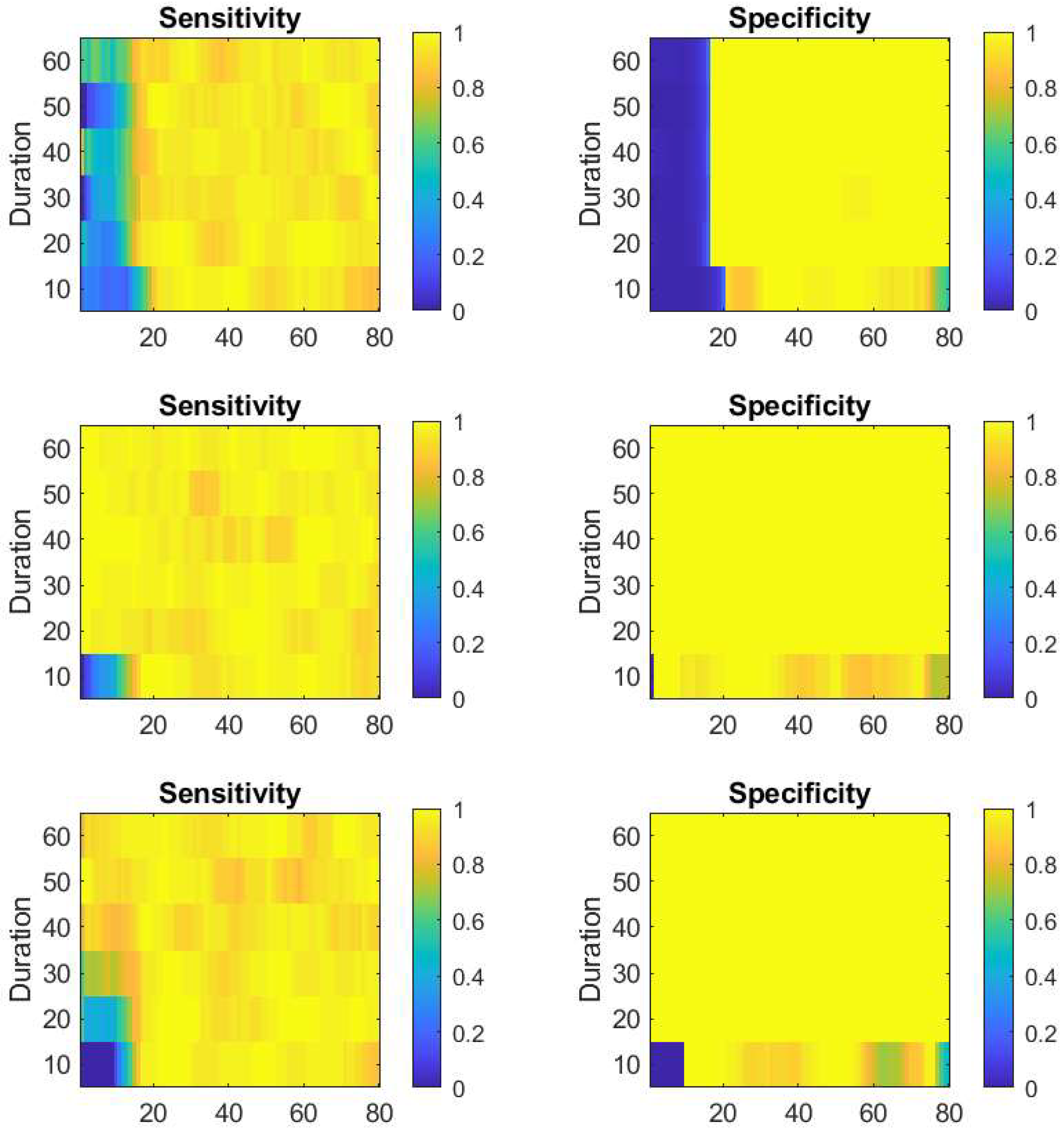
In the second experiment, we apply the reinforcement paradigm to generated seizures of different maximal length, ranging from 10 to 60 samples. In this experiment the other generation parameters were kept constant

{{T}_{s}

T_{n}

P_{s}, P_{n}} = {0.1,0.9,0.02,0.98}

and corresponding to low confusion factor (high separation) between the simulated normal and seizure states. Figure 10 presents the results.

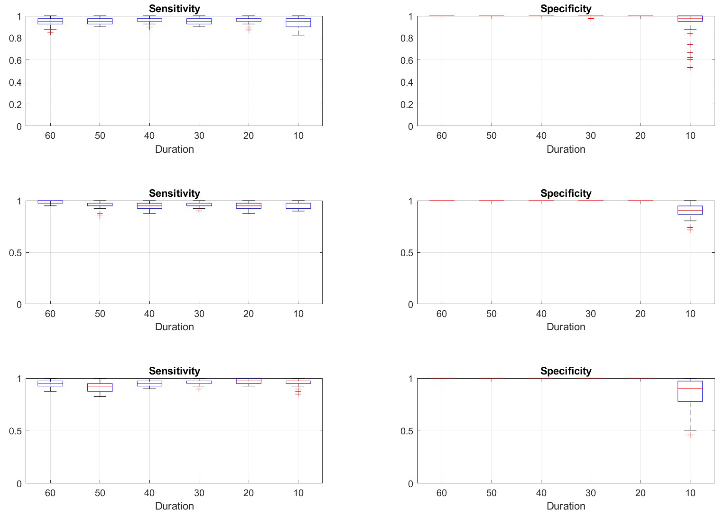
Also for this set of data, we show the sensitivity and specificity asymptotic behaviour by the boxplots on Figure 11.

4. Conclusions

As demonstrated in section 3.1 and visually presented on Figure 5, the proposed reinforcement parameter adaptation successfully converges to a detector with both high sensitivity and specificity performance. This is achieved from a variety of initial settings, some very “liberal”, allowing for many false positive detections, other very “conservative”, skipping some real events. In all cases, we use here the same event generation parameters. The later correspond to a relatively good separation between normal and seizure epochs with confusion factor of 0.062. We see from Figure 7 that for all initial values, the detector parameters reach approximately the same optimal levels due to the reinforcement algorithm. As the process is continuously active, certain fluctuation are present but the system recovers its target parameters and shows asymptotic stability.

To answer the question of how far we can trust the method with respect to the separation between seizures from normal periods, we have performed the experiments reported in section 3.2. From the results of the first test, shown on Figure 8 and Figure 9 we see that independently from the initial detection parameters, the reinforcement adaptation provides stable sensitivity for generation parameters corresponding to confusion factor less than 0.2. For the specificity, the adaptive process fails already for confusion factors greater than 0.1. The conclusion is that for systems with marginal or poor distinction between normal and seizure states, the detector can still adapt for proper detection of the events but will yield also false positive detections.

The final test explores the limits of the event durations that the approach will still be useful. From the results shown on Figure 10 and Figure 11, we see that again, the sensitivity reaches high values independently of the initial detector settings for all maximal event durations ranging from 10 up to 60 simulation steps. The specificity trace, however, is not stable for short seizure events. As in the previous test, we see that for short seizures, the algorithm will manage to restore an optimal detection but at the expense of letting through false positive detections.

5. Discussion

In this work, we first present a generic method for adaptive detection reinforcement. We call it TOREADA (topological reinforcement detection algorithm) and here we will explain the role of “topology”. In addition to the formal description in Section 2, a more intuitive insight might be helpful. Our major assumption, or axiom, is that the events that will be detected form within certain parameterization a connected continuous manifold. An ad-hoc detector setting, or the detection manifold, may cover partially the “true” event manifold, therefore resulting in false positive detections (FP) and false negative detections (FN) that count detected non-events and undetected true event correspondingly. Therefore the reinforcement process, or learning paradigm, is associated with deforming the detection manifold so that it can possibly cover as precise as possible the true event manifold. To do this, we introduce two complimentary transformations: Embedding and Envelope. The embedding step expands the detection manifold to an “embedding” one that contains the former. All events that fall into the larger, embedding manifold form the training set of events. In this way if initially the detector is not detecting events, they may still fall into the training set. The second stage is taking of the envelope around all classified true positive events. This step will form a “tighter” manifold within the embedding one that will possibly help to reject false positive detections. Finally we take the envelope manifold as the new detection manifold and subsequently the process is iteratively repeated according to appropriate schedule.

The two steps of embedding and taking an envelope are by far not unique. Taking a too wide embedding manifold around the current detection one, for example, may speed-up the process of reducing the FN events but at the same time it may introduce too many FP events that will make the assessment of the true events quite complicated. A very tight envelope may reduce the FP detections but will counter-act the embedding process and consequently will slow-down the reduction of undetected true events.

We have also left outside the scope of this work the procedure of validating the detected events. Here we allow for both supervised labelling or automated, using clustering algorithm for example, as proposed in our previous work [11]. Including this form of automated validation into the simulation tests will be a subject of our future research. Another extension of the current work will involve simulation of the optical flow output signals and not just the epi-factor. This will make possible testing our real-world adaptive algorithm, also presented in [11], that involves also the adjustment on the move of the frequency interval relevant for the particular seizure generating system. We remind that here our objective was to concentrate on steps described by equations (5) and (6).

The classic approaches to machine learning, including applications targeting detection of convulsive epileptic states, rely on available big collections of labelled data [15]. The belief there is that these collections contain the necessary information and that they can account for all the variability of the real-world scenarios. Our concept does not require, although it may use, a pre-recorded labelled sets of events. It acquires its training sets along with the operation of the detector and therefore is a continuous learning from experience paradigm. This way, the method is applicable to non-stationary situations and more generally, can potentially cope with the real-world variability of conditions. Moreover, in contrast to the static data collection paradigm, the TOREADA concept can potentially incorporate adaptive reinforcement of the data acquisition protocols. It can for example, adjust spectral ranges, apertures and other sensor properties in order to achieve optimal performance.

The above topological paradigm presents also certain restrictions. If the events that we are attempting to detect are of several different classes, corresponding to disconnected manifolds, our approach is unlikely to work. A possible solution would be to introduce multiple initial detection manifolds and apply the TOREADA algorithm to each one.

As a particular real-world application, we presented here also our system for convulsive seizures detection. This explicit example of TOREADA is an operational implementation undergoing field trials in clinical and care settings. We use here this realization, called also Dual Detection algorithm, to provide numerical validation and performance assessment of the generic concept.

We used in this work Monte Carlo (MC) type of numerically simulated data instead of collected clinical data. There are several reasons for this. First, validating and exploring the limits of adaptive and machine learning algorithms in clinical conditions may present certain ethical issues. If the alerting system runs out of optimal setting and fails to alert for a convulsive event, this may put the patient at risk. Conversely, if unsuccessful reinforcement trial leads to many FP alerts, the care personnel may switch the system off. Second, no amount of real-life examples can provide enough data for all possible scenarios and exceptions that the system may encounter elsewhere. Finally, the use of simulated data avoids the issues of privacy, especially present in the case of supervised validation of the video data.

Concerning our results in Section 3, we note again the “asymmetry” between the performance limits of our approach with respect to the sensitivity and specificity. Specificity is lost earlier with the decrease of seizure/normal separation, either due to confusion increase or seizure length decrease, as seen from Figure 8, Figure 9, Figure 10 and Figure 11. As mentioned earlier, it is a result of the “competition” between the embedding process described in this particular implementation by equation (5) and the envelope described by equation (6). Other choices, for example a more conservative embedding and tighter envelope may reverse the situation and the system will lose sensitivity while the reinforcement algorithm still achieves high specificity. To end this point, the current results are favourable in the view of clinical and care practice. The harm of undetected seizure events may be potentially higher than that of false alarming, without diminishing of course the need to reduce the later as further as possible.

Funding

Partially funded by “De Christelijke Vereniging voor de Verpleging van Lijders aan Epilepsie”. Program 35401, Remote Detection of Motor Paroxysms (REDEMP).

Conflicts of Interest

The authors declare no conflicts of interest, The funders had no role in the design of the study; in the collection, analyses, or interpretation of data; in the writing of the manuscript; or in the decision to publish the results.

References

Harden, C.; Tomson, T.; Gloss, D.; Buchhalter, J.; Cross, J.H.; Donner, E.; French, J.A.; Gil-Nagel, A.; Hesdorffer, D.C.; Smithson, W.H.; et al. Practice guideline summary: Sudden unexpected death in epilepsy incidence rates and risk factors: Report of the Guideline Development, Dissemination, and Implementation Subcommittee of the American Academy of Neurology and the American Epilepsy Society. Neurology 2017, 88, 1674–1680. [Google Scholar] [CrossRef] [PubMed]
Lamberts, R.; Thijs, R.; Laffan, A.; Langan, Y.; Sander, J.W. Sudden unexpected death in epilepsy: People with nocturnal seizures may be at highest risk. Epilepsia 2017, 23, 253–260. [Google Scholar] [CrossRef] [PubMed]
Herrera-Fortin, T.; Assi, E.B.; Gagnon, M.-P.; Nguyen, D.K. Seizure detection devices: A survey of needs and preferences of patients and caregivers. Epilepsy Behav. 2021, 114, 107607. [Google Scholar] [CrossRef] [PubMed]
Bruno, E.; Viana, P.F.; Sperling, M.R.; Richardson, M.P. Seizure detection at home: Do devices on the market match the needs of people living with epilepsy and their caregivers? Epilepsia 2020, 61, S11–S24. [Google Scholar] [CrossRef] [PubMed]
Geertsema, E.; Visser, G.; Sanger, J.; Kalitzin, S. Automated non-contact detection of central apnoea using video. J. Neural Biomed. Signal Process. Control 2020, 55, 101658. [Google Scholar]
Geertsema, E.; Visser, G.; Viergever, M.; Kalitzin, S. Automated remote fall detection using impact features from video and audio. J. Biomech. 2019, 88, 25–32. [Google Scholar] [CrossRef] [PubMed]
François-Lavet, V.; Henderson, P.; Islam, R.; Bellemare, M.G.; Pineau, J. An introduction to deep reinforcement learning. Foundations and Trends® in Machine Learning 2018, 11, 219–354. [Google Scholar] [CrossRef]
Sutton, R.S. Introduction: The challenge of reinforcement learning. In Reinforcement learning; Springer US: Boston, MA, 1992; pp. 1–3. [Google Scholar]
Wiering, M.A.; Van Otterlo, M. Reinforcement learning. Adaptation, learning, and optimization 2012, 12, 729. [Google Scholar]
Fayaz, S.A.; Jahangeer Sidiq, S.; Zaman, M.; Butt, M.A. Machine learning: An introduction to reinforcement learning. Machine Learning and Data Science: Fundamentals and Applications 2022, 1–22. [Google Scholar]
Kalitzin, S. Adaptive Remote Sensing Paradigm for Real-Time Alerting of Convulsive Epileptic Seizures. Sensors 2023, 23, 968. [Google Scholar] [CrossRef] [PubMed]
Kalitzin, S.; Petkov, G.; Velis, D.; Vledder, B.; Lopes da Silva, F. Automatic segmentation of episodes containing epileptic clonic seizures in video sequences. IEEE transactions on biomedical engineering 2012, 59, 3379–3385. [Google Scholar] [CrossRef] [PubMed]
Kalitzin, S.; Geertsema, E.; Petkov, G. Optical flow group-parameter reconstruction from multi-channel image sequences. In Frontiers of Artificial Intelligence and Applications Application of Intelligent Systems; Petkov, N., Strisciuglio, N., Travieso-Gonzalez, C., Eds.; IOS Press: Amsterdam, The Netherlands, 2018; Volume 310, pp. 290–301. [Google Scholar]
Binder, K. Introduction: Theory and “technical” aspects of Monte Carlo simulations. In Monte Carlo methods in statistical physics; Springer Berlin Heidelberg: Berlin, Heidelberg, 1986; pp. 1–45. [Google Scholar]
Yang, Y.; Sarkis, R.A.; El Atrache, R.; Loddenkemper, T.; Meisel, C. Video-based detection of generalized tonic-clonic seizures using deep learning. IEEE J. Biomed. Health Inform. 2021, 25, 2997–3008. [Google Scholar] [CrossRef] [PubMed]

Figure 1. “Category” representation of the TOREADA approach to reinforcement. Green blocks represent the input and the output of an automated system. The blue block “Decision Manifold” represents a direct, without any adaptive reinforcement, reactive process. The reinforcement learning loop consists of an embedding (brown oval “Embedding”) step where the decision criteria are relaxed and define the “Observation Manifold”(blue box) in order to account for a larger variety of input events, the training data. An assessment procedure (brown rectangle “Assessment”) that can be either supervised or automated, labels the events as true or false (blue box “Labelled Data”). The labelled set of events provides input for constructing an envelope of decision criteria (brown oval “Envelope”) that optimizes the detection of the true events and the rejection of the false ones. This decision envelope forms the reinforced, adapted new decision manifold.

Figure 2. Illustration of the quantities used in the seizure-detection decision algorithm. The vertical axis represents the output of the optical flow and filtering pre-processing. The horizontal axis is the running time. Dashed blue line is the selected threshold and the blue arrow on the top is the selected observation elapsed time, or the detection depth. The grey box represents the pre-convulsive seizure onset (most typically the tonic phase) and the yellow area is the observed convulsive, clonic phase.

Figure 3. Generic scheme for Monte-Carlo type of simulating epi-marker. The output signal, the synthetic epi-marker, is generated according to a probabilistic model that determines the distribution of values at each time depending whether the system is in a pre-defined ictal (seizure) state of in a “normal” state.

Figure 4. Real (top frame) and synthetic (bottom frame) Epi-marker. On both plots, the Epi- marker is the blue trace and the vertical axes indicate its values. Note that the negative values on the top frame are due to conveniently introduced offset as compensation for white noise background. The horizontal axes on both plots represent the real and simulation time (sample steps) correspondingly. The vertical red line on the top frame represents the beginning of the seizure as detected in real time by the detector. On the bottom frame, the two red lines are at the beginning and the end of the model seizure event; the red star is the detected onset by the algorithm.

Figure 5. Results from simulations of the reinforcement procedure starting from various initial detector settings. Left plot is the sensitivity presented in pseudo-colour code from the colour bar. The vertical axis is the trial number; the corresponding parameters are in Table 1. The horizontal axis is the epoch number (each epoch of 3600 simulation steps, see section 2.5) from the start of the simulation experiment. The right plot is with the same notations but showing the specificity evolution.

Figure 6. Statistical distributions of sensitivity (left plot) and specificity (right plot) derived from the last 50 epochs of the simulations of reinforcement procedure starting from various initial detector settings, same data as shown on Figure 5. The vertical axes are the corresponding quantities, the horizontal represent the number of initial parameters given in Table 1. The boxes are the 25%-75% percentiles, the red lines are the median values, and the whiskers denote the 5%-95% percentile values and the red crosses are the outliers. .

Figure 7. Traces (black lines) of the detector parameter adaptation from simulations of the reinforcement procedure starting from various initial detector settings. The horizontal axis is the epoch number (each epoch of 3600 simulation steps, see section 2.5) from the start of the simulation experiment. The labels on the vertical axes denote the corresponding parameter.

Figure 8. The notations are the same as on Figure 5. Each row of images represent a session with different initial detection parameters given in Table 2. For better inspection of the results, he vertical axes are showing the confusion factor from eq. (10) associated with the content of Table 3.

Figure 9. Statistical distributions of sensitivity (left column of plots) and specificity (right column of plots) derived from the last 50 epochs of the simulations of reinforcement procedure starting from three various initial detector settings (each horizontal line of plots) given in Table 2, same data as shown on Figure 8. Vertical axes are the quantities; the labels on the horizontal axes indicate the various confusion factors as given in Table 3. The boxplot features are the same as on Figure 6.

Figure 10. The same notations as in Figure 6. The vertical axes here represent the simulated maximal seizure duration in simulation steps. The three line of images correspond to the three different initial detection parameters from Table 2.

Figure 11. Statistical distributions of sensitivity (left column of plots) and specificity (right column of plots) derived from the last 50 epochs of the simulations of reinforcement procedure starting from three various initial detector settings (each horizontal line of plots) given in Table 2, same data as shown on Figure 10. Vertical axes are the quantities; the labels on the horizontal axes indicate the various maximal seizure lengths. The boxplot features are the same as on Figure 6.

Table 1. Initial values of the detector parameters before starting reinforcement learning. First column is he trial number, the second: detection threshold, third: the detection window length the forth: the minimal number of values above the threshold for detecting a seizure event. The fifth column is the blackout period, taken the same (90 samples) throughout all simulations.

Trial No	Threshold	N	n	Black-out
1	0.1	10,00	9,00	90,00
2	0.2	8,00	7,00	90,00
3	0.3	6,00	5,00	90,00
4	0.4	7,00	6,00	90,00
5	0.5	10,00	9,00	90,00
6	0.6	8,00	7,00	90,00
7	0.7	6,00	5,00	90,00
8	0.8	5,00	4,00	90,00
9	0.9	4,00	3,00	90,00

Table 2. Three different initial detection parameters used for the two experiments in this section. The columns are the same as in Table 1.

Session	Threshold	N	n	Black-out
1	0.2	5	3	90
2	0.5	10	9	90
3	0.8	10	10	90

Table 3. Seizure generation parameters for the first experiment in this section. The first column is the trial number, second: the threshold of normal state, third: the threshold of simulated seizure state, forth: probability of exceeding the threshold in normal state, fifth: probability of exceeding the threshold during seizure state. The fifth column is the confusion factor for the corresponding generation parameters as give in equation (10). In this experiment, the maximal seizure duration is always 60 samples.

Trial No	$T_{n}$	$T_{s}$	$P_{n}$	$P_{s}$	C
1	0,1	0,9	0,02	0,98	0,02
2	0,4	0,6	0,1	0,96	0,064
3	0,3	0,4	0,1	0,9	0,1
4	0,2	0,4	0,15	0,75	0,17
5	0,4	0,5	0,2	0,7	0,24
6	0,5	0,5	0,3	0,6	0,35

Disclaimer/Publisher’s Note: The statements, opinions and data contained in all publications are solely those of the individual author(s) and contributor(s) and not of MDPI and/or the editor(s). MDPI and/or the editor(s) disclaim responsibility for any injury to people or property resulting from any ideas, methods, instructions or products referred to in the content.

© 2024 by the authors. Licensee MDPI, Basel, Switzerland. This article is an open access article distributed under the terms and conditions of the Creative Commons Attribution (CC BY) license (http://creativecommons.org/licenses/by/4.0/).

Copyright: This open access article is published under a Creative Commons CC BY 4.0 license, which permit the free download, distribution, and reuse, provided that the author and preprint are cited in any reuse.

Alerts

MDPI Initiatives

Important Links

Choose an area of interest and we will send you notifications of new preprints at your preferred frequency.

Disclaimer

Topological Reinforcement Adaptive Algorithm (TOREADA) Application to Alerting of Convulsive Seizures and Validation with Monte-Carlo Numerical Simulations

Abstract

Keywords:

Subject:

1. Introduction

2. Materials and Methods

2.1. General Concept of TOREADA

2.2. Detection of Convulsive Seizures

2.3. Dual Detection Approach

2.4. Generating Synthetic Data

2.5. Simulation Protocol and Performance Quantification

3. Results

3.1. Static Seizure Generation Scenarios and Various Initial Detector Parameters

3.2. Change of Seizure Generation Parameters

4. Conclusions

5. Discussion

Funding

Conflicts of Interest

References

MDPI Initiatives

Important Links

Subscribe