A. INTRODUCTION
A1. THE THERMAL STIMULATED DEPOLARIZATION (TSD) AND THE THERMAL-WINDOWING DECONVOLUTION (TWD) CHARACTERIZATION TECHNIQUES. A BRIEF INTRODUCTION.
Originally, thermal stimulated current depolarization techniques were used to measure charge detrapping in low-molecular-weight organic and inorganic non-conductive compounds. Ever since 1967 they have been applied to the study of structural transitions in polymers, another class of non-conductive materials. The credit for the initial development must be given to C. Lacabanne at the University of Toulouse, France [
1], J. Vanderschueren at the University of Brussels, Belgium [
2], and J. Van Turnout of the University of Handoven in Holland [
3], who applied thermal stimulated depolarization methods to the investigation of the microstructure and properties of polymers. The result of their 20 years of dedicated research has led to the publication of hundreds of articles in the leading scientific journals . Additionally, Lacabanne pioneered in 1974 the use of the polarization –depolarization procedural technique she called “Thermal -Windowing Spectroscopy”, successively renamed over the years “Relaxation Map Analysis (RMA)” in 1993 [
4] and more recently "Thermal-Windowing-Deconvolution" (TWD) in 2022 [
5], and applied it to the study of a wide variety of macromolecular materials, synthetic and organic [
6]. The use of "thermal-windowing" rendered possible the deconvolution of the thermal stimulated depolarization peaks and the decoupling of the relaxation modes responsible for internal motion permitting, for the 1
st time, a better understanding of their coupling characteristics which relate to the state of the material itself, in particular its thermodynamic sensitivity to “internal stress”.
The methods of thermal stimulated depolarization became very popular in the early 90’s as a result of the introduction by Solomat Instruments (Stamford, CT, USA) of the automated TSD/TWD spectrometer on the thermal analysis market [
4]. At Solomat, where this author was the Director of Research, these dielectric spectrometers were called TSC/RMA, and a book was published as a guide for the use of the spectrometer and the analysis of the results to promote the sales of the TSC/RMA spectrometers [
4]. This new technology could "measure up" the amorphous state in such diverse applications as bonding and cohesion between matrices and fibers for composites, between metals and paints, between the crystalline phases in semi-crystalline polymers or even between the phases in a blend or a block copolymer. In 2022, a new book on the same TSD/TWD subject was published [
5] with a different objective in mind: explain the depolarization results using our new Dual-Phase model approach of describing the interactions in polymers by application of the Grain-Field Statistics. This new book provides a different interpretation of the results obtained by TSD and TWD, while the book of 1993 [
4] provided the classical formulation of Lacabanne [
1], Vanderschueren [
2], and Van Turnout [
3]. In particular, we develop in [
7], in response to a question raised in [
8], a new understanding of the amorphous state of matter submitted to an electrical field using the variables that enter the dynamic equations of the Dual-Split statistics when it is brought out of equilibrium by such thermal mechanical processing procedures as to induce dissipative structures (Rheomolding [
9], Rheo-Fluidification and Sustained-Orientation [
10].
Our general objective is to explain all the properties of polymers using a new statistical formulation of their interactions: “the Grain-Field Statistics of Dissipative systems”. The application to the rheology of polymer melts has been introduced [
11,
12] and is the subject of a specific publication [
13]. In the case of the dielectric properties, in [
5] and in this article, the subject of the polarization and depolarization of the dipoles and the creation of space charges is studied from a different angle than the traditional views [
1,
2,
3]: Is it possible (or not) to correlate the parameters of the Grain-Field Statistics to the thermo-kinetics features observed in a relaxation map of interactive dipoles: the compensations and super-compensation lines and their comprehension in terms of the Dual-Phase model [
7]?.
Sophisticated thermal analytical equipment are available on the market: Differential Scanning Calorimeters (DSC), Dynamic Mechanical Analyzers (DMA), dielectric spectrum analyzers (DEA), but none can characterize the amorphous state to determine the interactive coupling molecular basis for its non-equilibrium characteristics, either in the solid or in the molten temperature regions.
The 1st book of 1993 narrated how industry engineers and scientists would welcome the arrival of an instrument to tag and measure the internal stress in injection molded, extruded or blow molded parts, or capable of characterizing the segregation in a blend or a block copolymer, or determining the bonding strength of paints and glues. The book explained that Lacabanne, Vanderschuren and Van Turnout had developed the basic technology for such an instrument. Solomat Instruments LLP sought and obtained a license to develop, manufacture and commercialize the new technology. The result was the first automated TSD/TWD Spectrometer that started to sell in late 1988.
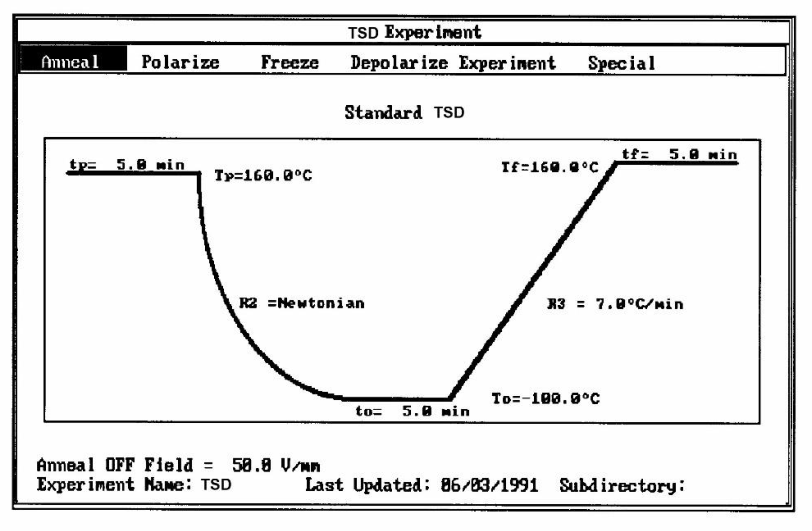
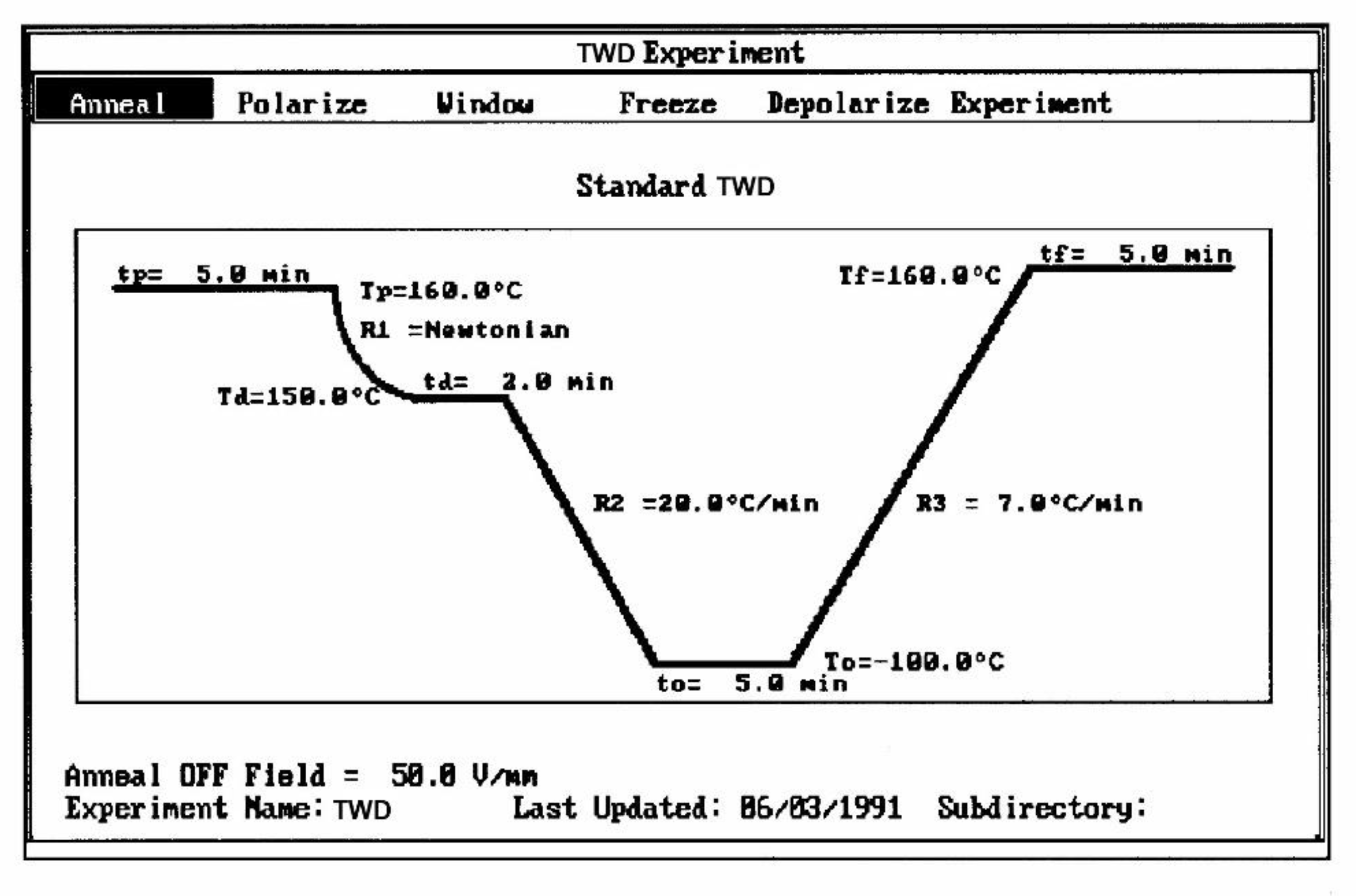
Several techniques exist to analyze the molecular response of materials to physical or chemical inputs, in order to determine their specific performance. Differential Scanning Calorimetry (DSC), and Differential Thermal Analysis (DTA) are among the most popular in laboratories and on production sites. Other techniques include Thermal Mechanical Analyzers (TMA), Dynamic Mechanical Analyzers (DMA), stress relaxation or creep analyzers, thermal expansion coefficient devices, and dielectric analyzers (DEA). The method of thermo-stimulated depolarization (TSD) consists in putting the specimen rapidly at high temperature (above the transition temperature at which the relaxation phenomena is expected), orient the dipoles at that temperature and freeze-in the orientation thus produced by quenching at low temperature (
Figure 1).
The voltage field applied is then removed and the temperature is ramped linearly back up to reveal the polarization induced at high temperature. TSD is therefore a thermally stimulated recovery experiment. An electrometer is connected to the sample to record the short-circuit current while heating . A current is created when the material depolarizes. This thermally stimulated depolarization current reveals the molecular mobility of the material's structure. The rate of depolarization is related to the relaxation times of the internal motions providing a new opportunity to study the physical and morphological structure of materials.
The depolarization current, J, flowing through the external circuit is measured by a very sensitive electrometer (capable of measuring currents 10 million times smaller than those measured by a tunneling microscope), and allows determination of the "dipole conductivity".
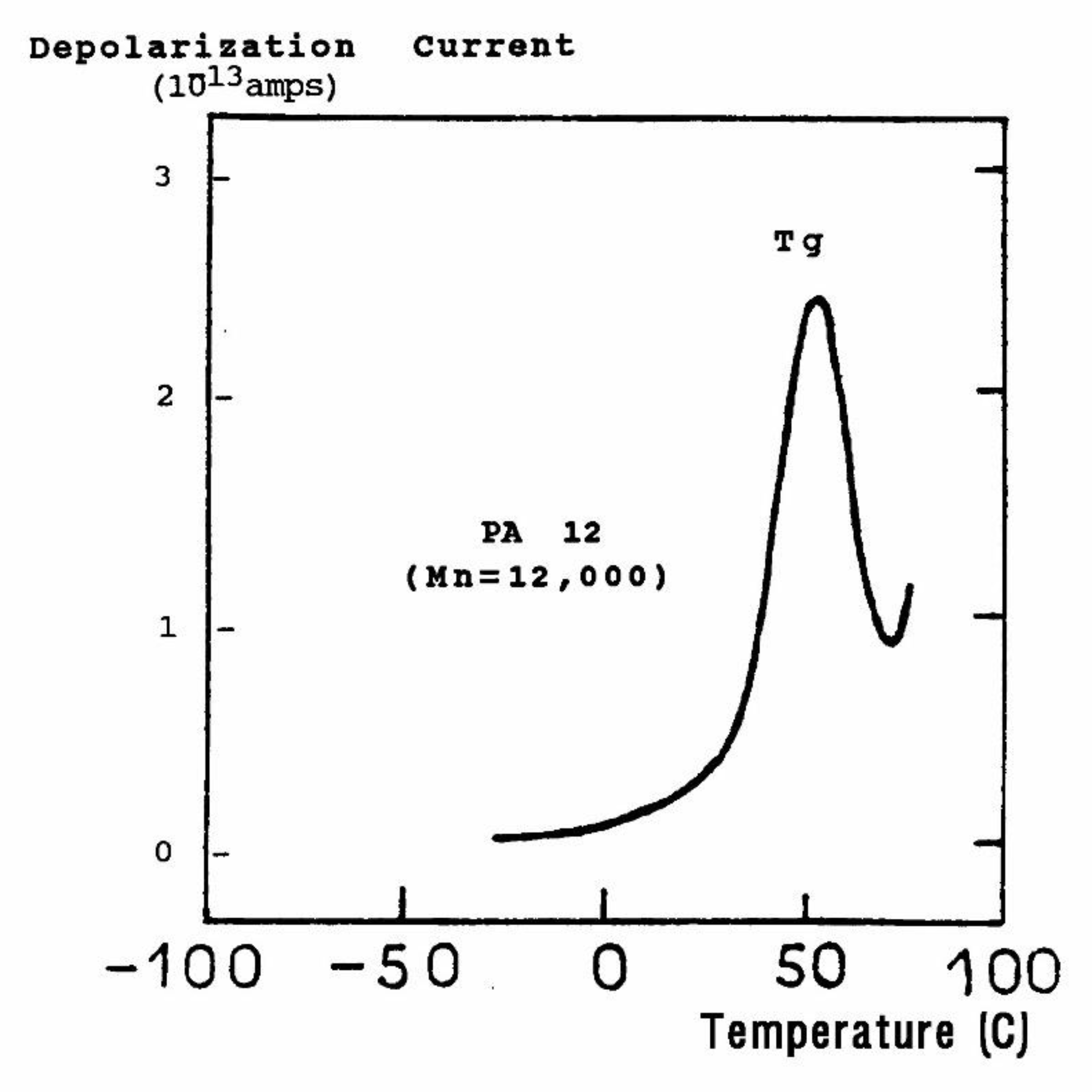
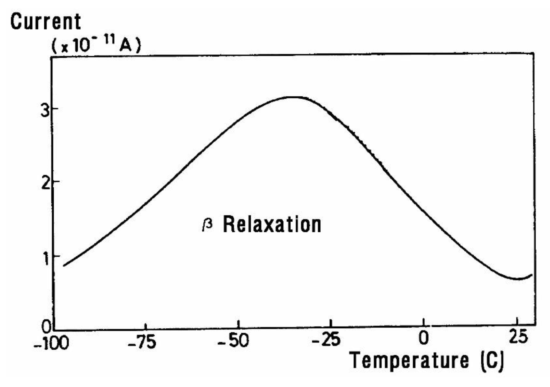
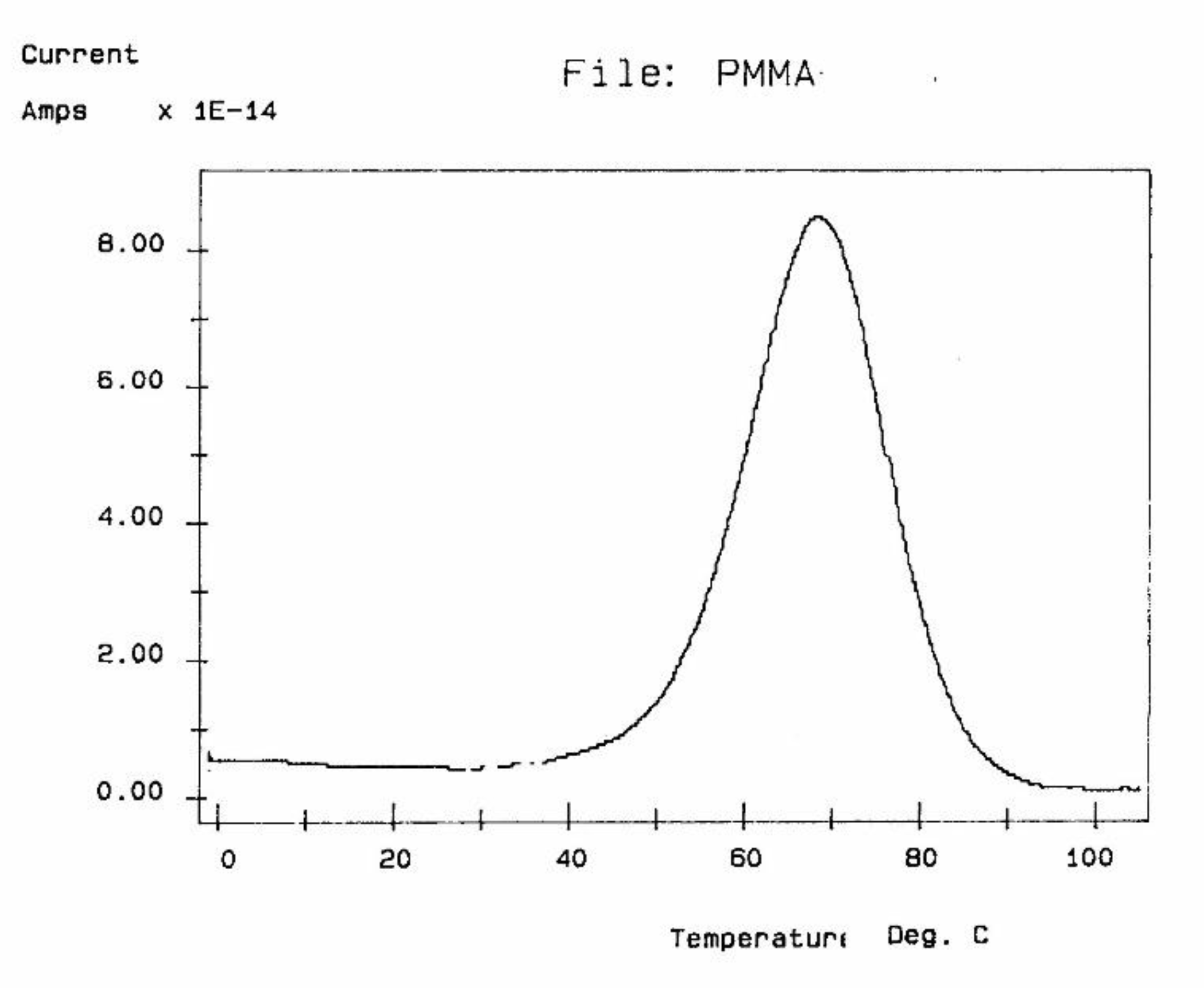
The current peaks recorded this way (
Figure 2a and
Figure 2b) are found to correlate well with the transition temperatures measured by mechanical relaxation (DMA), by DSC or by conventional (a.c.) dielectric spectroscopy (DETA). A TSD output looks like a tan δ versus temperature plot, showing maxima at the transitions occurring inside the material. In fact, TSD provides very similar results to those obtained from other analytical instruments operating at the same low frequency equivalent (10
-4 Hz), with the addition of an accrued sensitivity, and a separating power unseen in other technologies.
The concept of "thermal-windowing" gives the TSD another dimension. It consists of polarizing only a fragment of the full spectrum of relaxation and depolarizing it partially to isolate or "window" a single relaxation process. There are two types of possible windowing techniques: the first method, which can be called "partial isothermal recovery" or "isothermal windowing", consists of the following: first, polarize the sample at temperature Tp for a time tp adjusted to allow orientation only of a certain fragment of the dipoles. At the same temperature Tp, cut off the polarizing voltage and stay at Tp for a time td. This allows the depolarization of a fragment of the oriented dipoles. Finally, quench the sample to To << Tp. Reheat at constant rate and measure the current of depolarization. Δt = (tp - td) is the "time-window" and can vary between 1 min and about 1 hour.
The 2
nd commonly used thermal deconvolution method is the "thermal-windowing deconvolution experiment (
Figure 3), which we designate TWD in this book. TWD essentially gives identical results as the 1
st deconvolution method, yet it is faster to practice. In this option, a constant voltage is applied at Tp for a time tp, commonly of the order of 2 minutes. The temperature is then lowered to Td at which the voltage is removed and the specimen allowed to recover partially for a time td, usually equal to tp. ΔT = (Tp - Td) is the temperature window and can vary between 1° and about 10°C. The specimen is then quenched by 50° to 100°C to a sub-temperature T
o where the amount of polarization induced in the material is frozen. A linear heating-up is then performed, and the variation of current due to thermally induced depolarization or other current discharges is observed as a function of time (i.e. temperature). Since the current, J(t), is the derivative of polarization, the ratio P(t) divided by J(t) is a quantity with the dimension of time and represents, according to Bucci et al [
14,
15], the elementary relaxation time τi typical of the relaxing system.
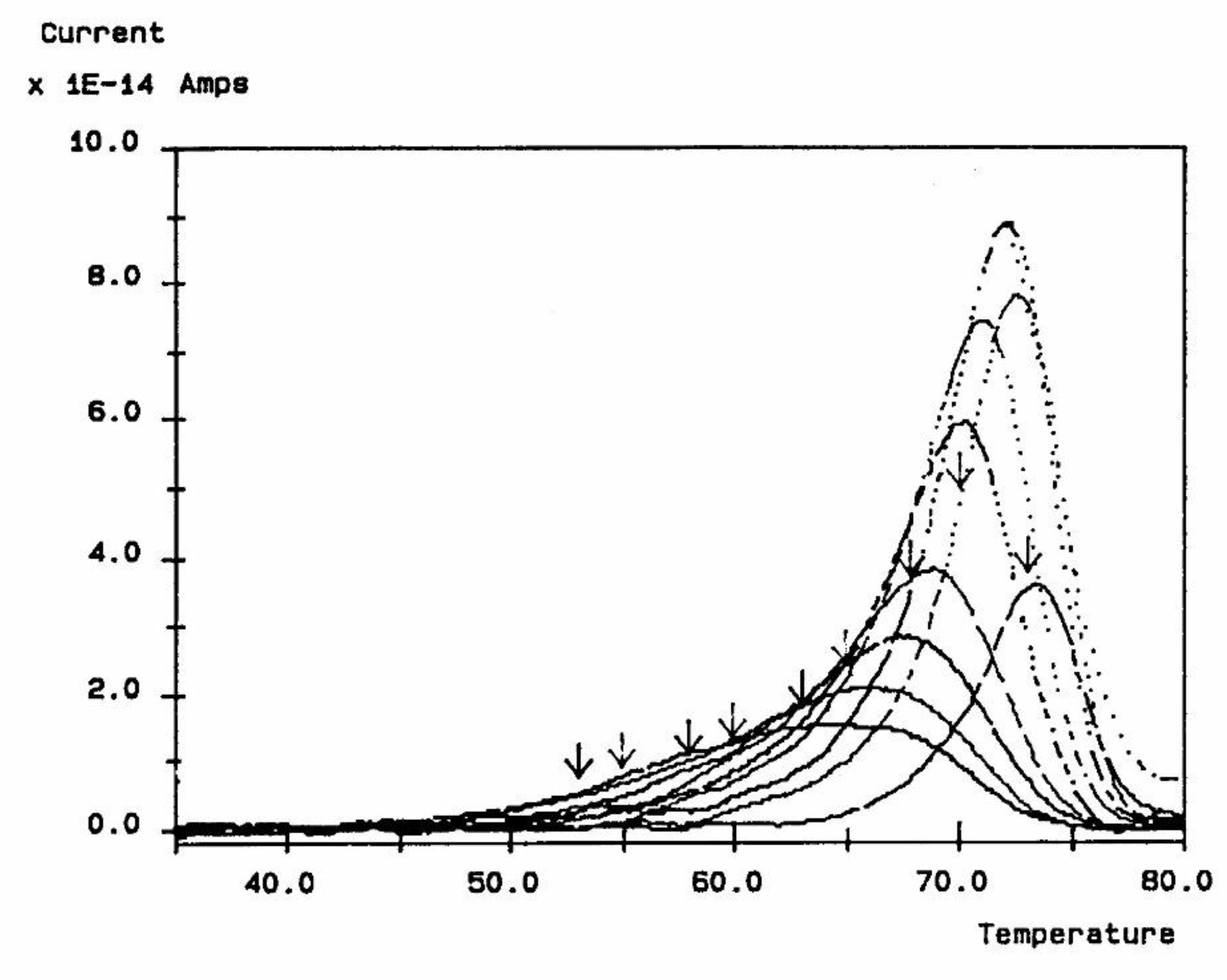
Figure 4 shows the result of thermal-windowing on the TSD output.
When tp, td, and (Tp - Td) are conveniently chosen, the depolarization current is supposed to represent the relaxation of a single Debye relaxation mode isolated from the spectrum of relaxation modes. By varying the value of the temperature of polarization Tp, and repeating the above thermal-windowing process, one can isolate the elementary modes one by one (
Figure 5).
The computer in the automated TSD/TWD spectrometer of Solomat integrated the current
vs temperature peak for each temperature, and calculated the value of the relaxation time at each temperature. According to the Bucci's equation ([
14,
15]; also p. 7 and 34 of [
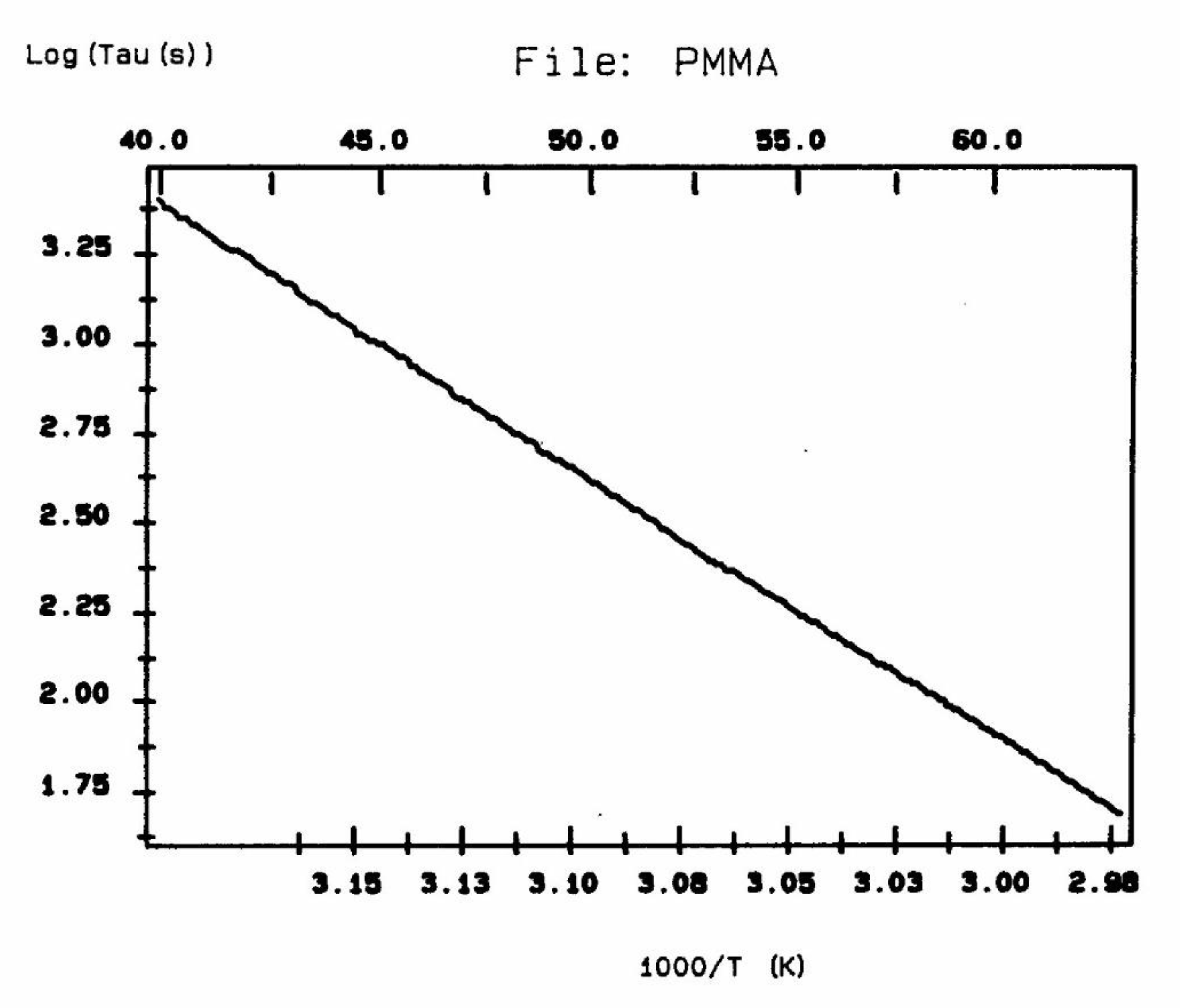
5]), the analysis of each resolved Debye peak obtained at various polarization temperature gives a temperature dependent retardation time τ
i(T) which often follows an Arrhenius dependence (
Figure 6).
According to Lacabanne [
1], the relaxation time in
Figure 6 is the inverse of the frequency of jump between two activated states of the depolarization process, the intercept of the Arrhenius equation is proportional to the Entropy of activation for the activated process involved, and the slope is proportional to the Enthalpy of activation. If a structure is "loose", the contrary of "ordered" or "compact", i.e. when molecular mobility is less hindered by the interactive intra-intermolecular surrounding, the Entropy of activation will be "larger". Conversely, any parameter which acts to "organize" the structure and create a tighter environment for the bonds will cause a decrease of the Entropy of activation. So, the activated Entropy calculated from the intercept of
Figure 6 gives an indication of "the degree of disorder" (DOD) of the structure [
16].
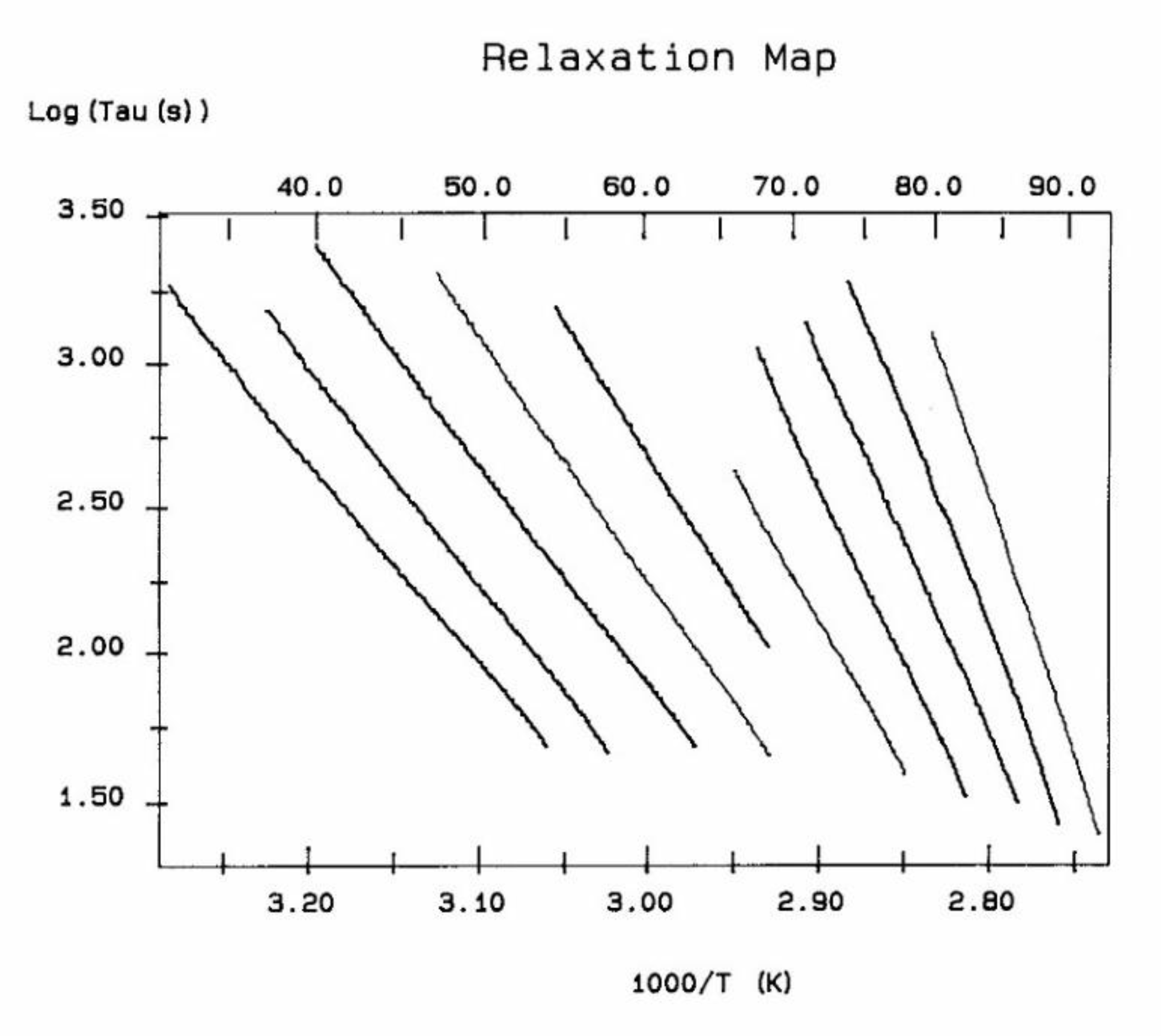
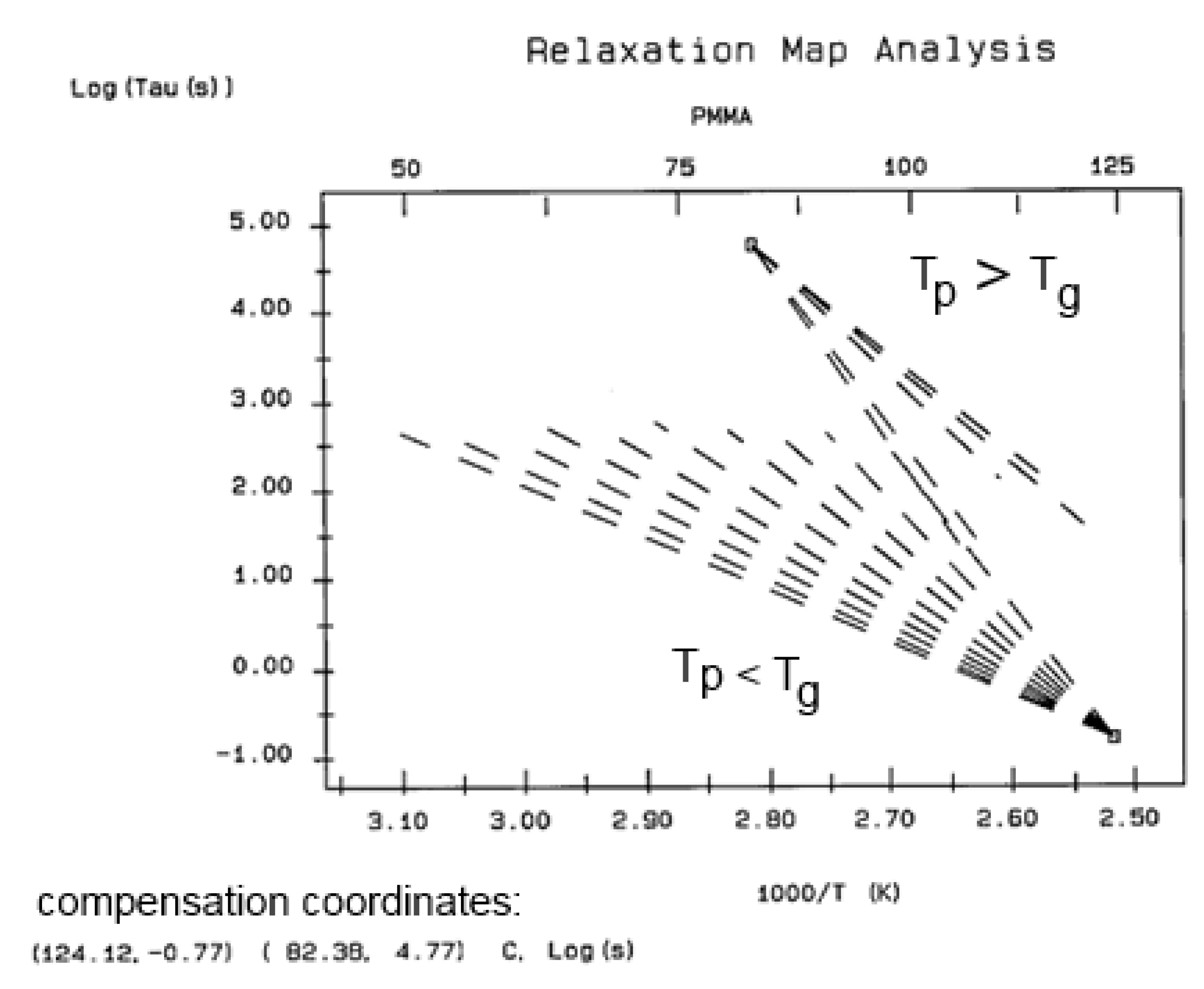
A relaxation map (
Figure 7) is obtained from a TWD experiment: it is the collection of the relaxation lines obtained for each deconvoluted Debye peak, and analyzed according to Bucci's equation. While the techniques based on Thermal Stimulated Depolarization, even when named using various other designations than TSD, were popular to characterize molecular motions in all kinds of non-conductive materials [
1,
2,
3,
4,
5,
6] , the TWD technology leading to a Relaxation map appears to be more specifically suited to determine the degree of cooperativeness between the relaxation modes responsible for internal motions at the main transitions, revealing the state of their structure and their morphology [
5,
16]. Relaxation maps can be looked at as "fingerprints" of the material, being representative of its chemical structure, morphology, and non-equilibrium structure (
Figure 8).
The analysis of the relaxation map determines the elementary Enthalpies of activation, and the pre-exponential factors (related to the Entropy of activation) for all the relaxation modes obtained by varying the temperature of polarization Tp.
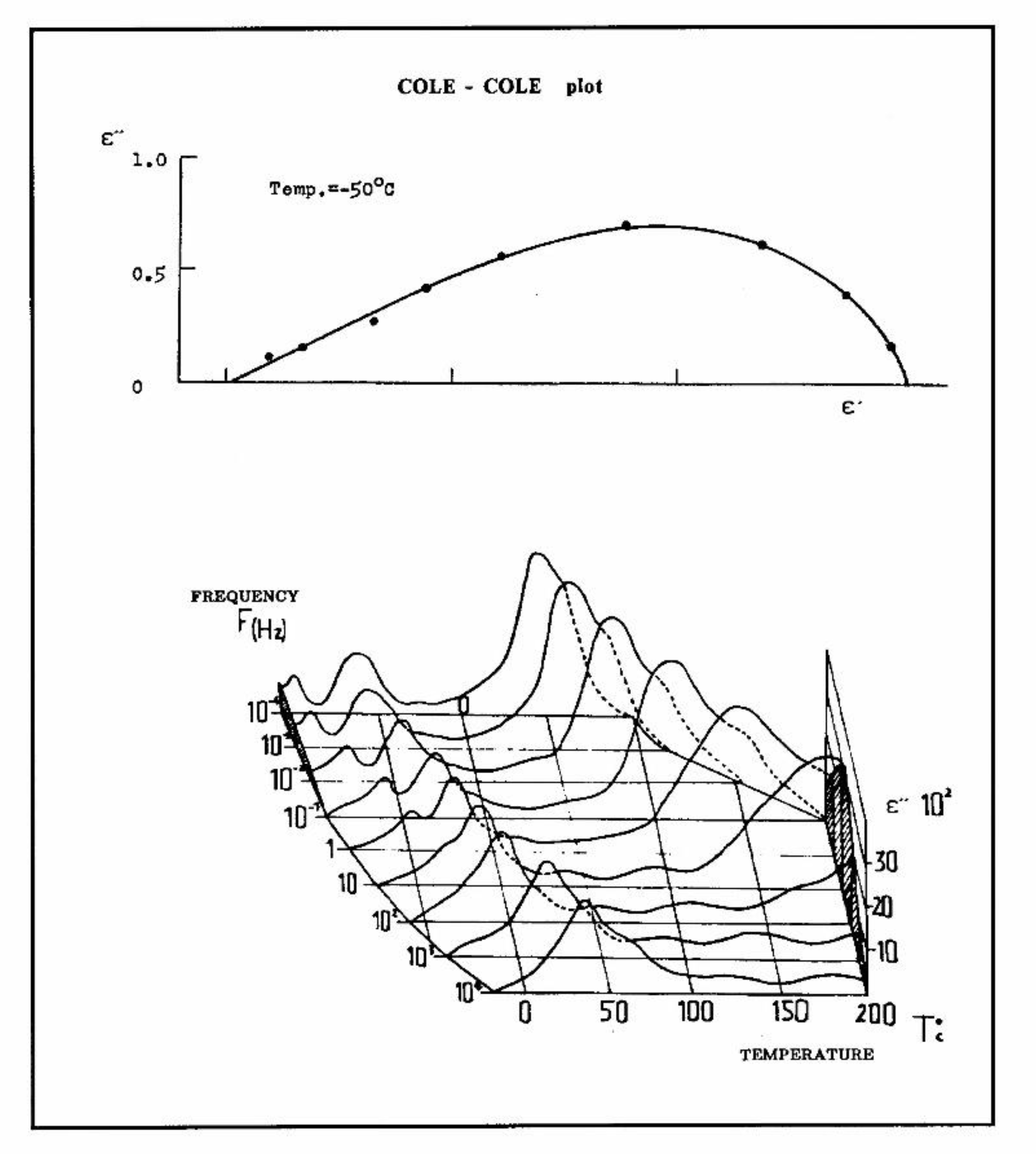
In summary, the relaxation observed during the recovery stage of TSD reveals the kinetics, and the powerful method of "thermal-windowing deconvolution” (TWD) deconvolutes the individual relaxation modes. This allows the study of their coupling characteristics, reflecting the structure and the physical state of the material. Constitutive equations can be used thereafter to reconstruct the material dielectric behavior (
Figure 9) by calculation of the fundamental physical parameters from the spectrum of relaxation (dielectric permittivity, etc) .
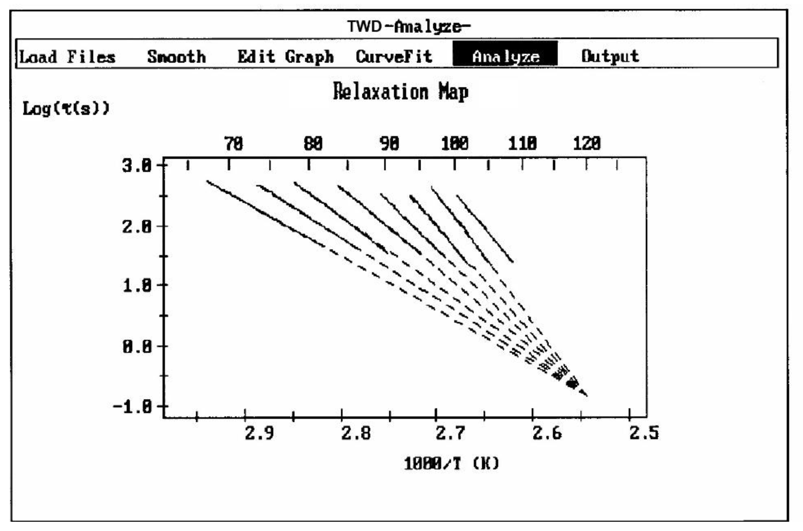
The various Arrhenius lines obtained by thermal-windowing at different polarization temperature, Tp , often converge to a common point, the compensation point (
Figure 10).
The spectral lines in
Figure 10 apply to a thermo-electrical activation of the dipoles below Tg (Tp < Tg), which results in a “positive” compensation: this means that the temperature of the compensation point is located above Tg and the convergence points downwardly. When Tp > Tg but below TLL , the spectral lines converge upwardly and backward to a compensation point located below Tg: the compensation is designated “negative” . An example is shown in
Figure 11. When Tp > TLL the spectral lines are parallel to each other and thus no longer converge (for an amorphous state at or near equilibrium) and they may no longer display an Arrhenius behavior (their spectral line is curved).
The coordinates of the compensation points, either positive or negative, can be found by a “compensation search”, a plot of the intercept versus the slope of the Arrhenius spectral lines . The compensation is validated when the plot in the compensation search (called a compensation line) is linear. In such a case, the dipoles are not independent in their relaxation, they are “interactively coupled”, the meaning of which is defined and specified in this review. The coordinates of the compensation points are calculated from the slope and the intercept of the compensation line. When the dipoles are not interactively coupling, i.e. when their motions are independent, their spectral lines are parallel and there is no compensation point in the compensation search. This lack of interactive coupling occurs above the TLL transition under equilibrium conditions .
It should be noted that there are several types of representation of the state of interactive coupling of an amorphous phase, the Relaxation Map of Log τi vs 1/T in
Figure 11 being one of them. For instance, when the relaxation time τi of each mode is converted to its Eyring form, τι
(Eyring) , we obtain an “(Eyring Relaxation Map) pursuant to the following equation (Eq. 2.5 of Ref. [
5]):
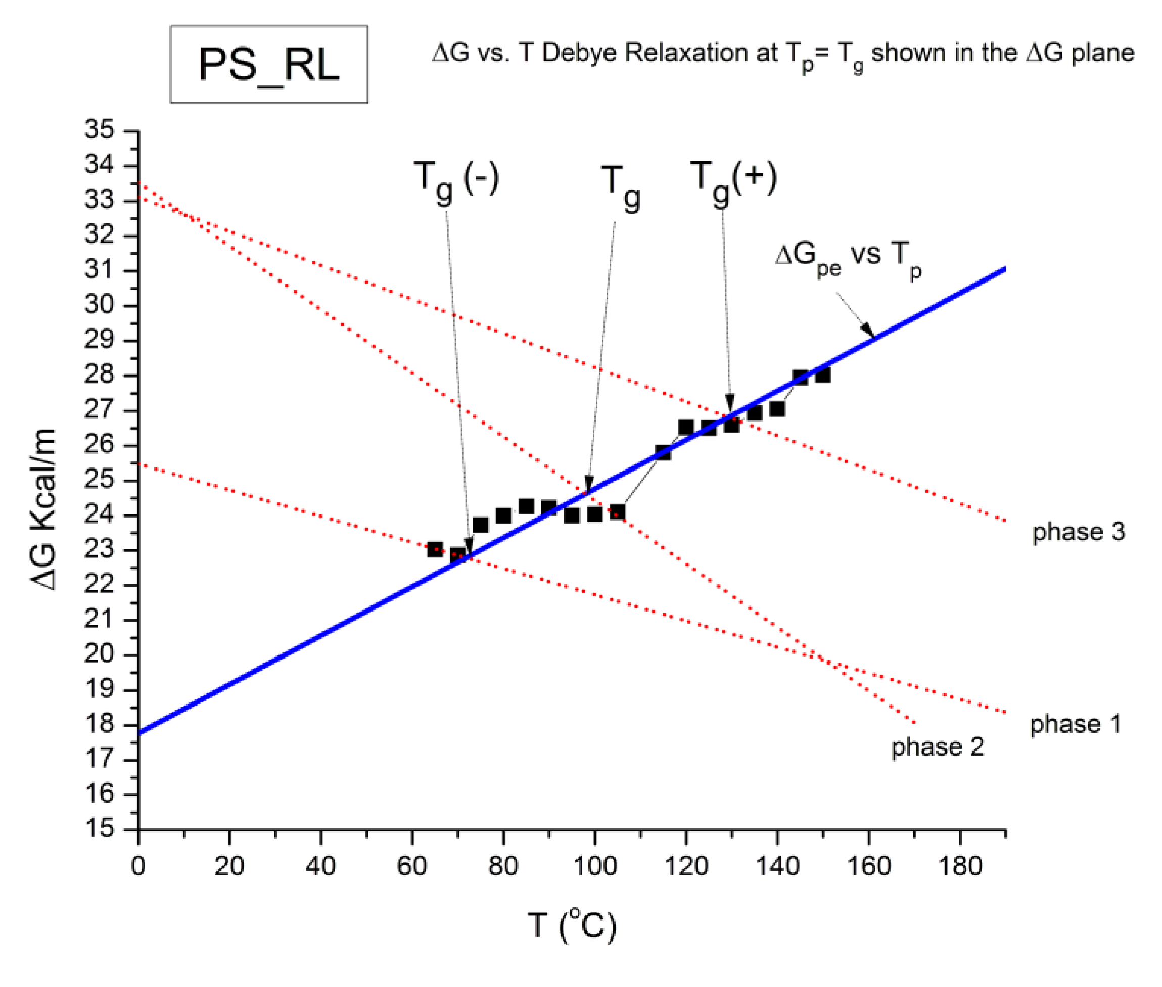
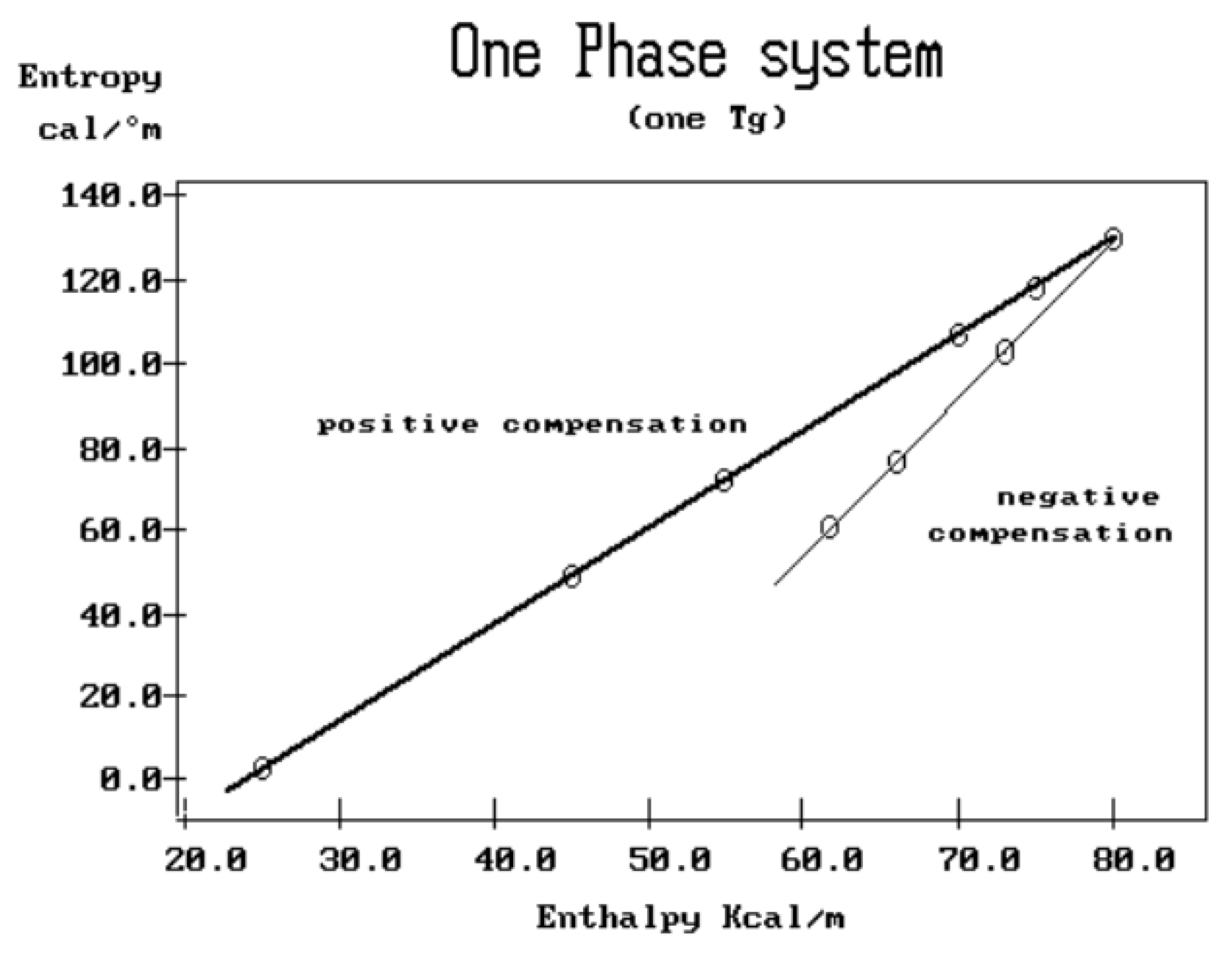
where h and k are the Planck and Boltzmann constants, respectively, and ΔHp, ΔSp are the enthalpy and entropy of activation of the Debye elementary relaxation modes at T= Tp. The relaxation data can also be presented in the ΔG vs. T plane where all the Eyring relaxation times are converted into ΔGi relaxation spectral lines : ΔG(T)= ΔHp-T ΔSp where T, the x-axis, is the temperature
during the depolarization stage (see Figure 2.7 of Ref. 5, p. 71). The compensation search in the ΔG plane consists of a plot of ΔSp vs. ΔHp, as illustrated in
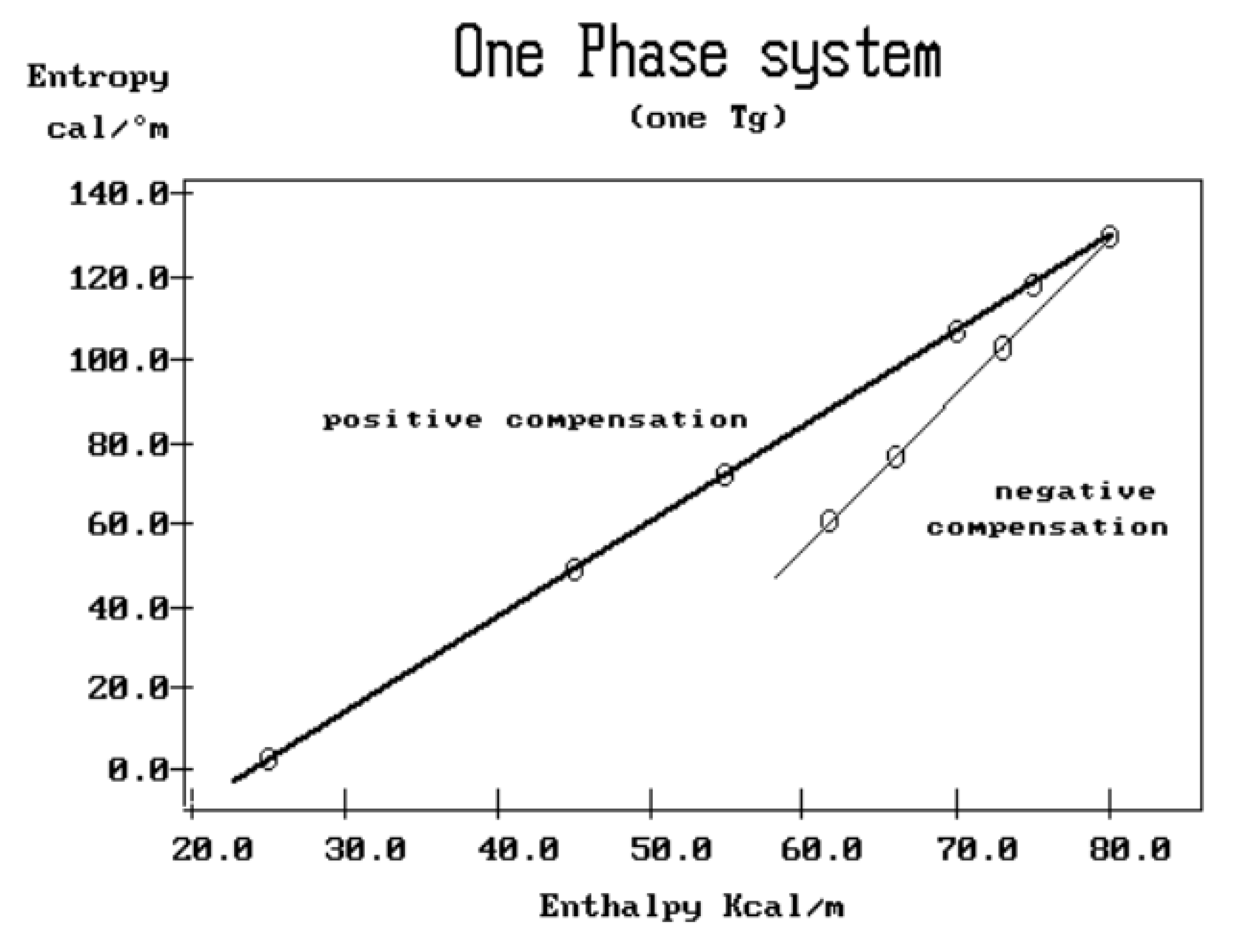
Figure 12 for an amorphous polymer exhibiting a single Tg transition, “a one phase system”.
In conclusion, the interest in thermal stimulated processes outcomes lies around this phenomenon of compensation, the determination of the coordinates of the compensation points , the interpretation of its origin, its practical use to characterize the degree of coupling in the amorphous phase of polymeric matter, and its relationship with the state of (non) equilibrium [
16]. In our opinion, a new type of thermal analysis was born with the introduction of the "thermal-windowing deconvolution" experimental procedure (TWD), which apparently permits to isolate , i.e. filter out, one by one, the single elementary Debye peaks that constitute the global depolarization peaks during the heating stage (
Figure 5).
The purpose of this review is to clarify the general description of TWD stated above, i.e. discuss and challenge the consensual understanding that a spectrum of elementary relaxation modes coexist in global TSD peaks and that the technique of TWD can deconvolute single Debye peaks from them. The challenge is to understand the compensation of the elementary relaxations, either the positive or negative compensations, and determine the meaning of the “interactive coupling” between these elementary relaxation motions extracted from global peaks. In other words, to simplify the true fundamental issue behind this research: is the deconvolution of global depolarization peaks into relaxation maps of compensating single Debye relaxations a sophisticated curvefitting procedure or is it fundamentally revealing the dual-phase and dissipative nature of the interactions in polymers? In order to better position this issue, we need to briefly review some of the assumptions of the model of Dual-Split kinetics (EKNETICS) that serve as the foundation of our development of the Dual-Phase Open Dissipative System Perspective ( [
7], [
10,
11,
12,
13]).
A2. INTRODUCTION TO THE DUAL-SPLIT KINETICS MODEL (EKNETICS).
It is not our intention to present here the details of our model of the physics of interactions in polymers. The interested reader can refer to an introduction of the Dual-Phase and Cross-Dual-Phase models of polymer physics interactions in references [
10,
12,
13,
17,
18]. We will limit ourselves in this text to presenting the general principles and fundamentals of the theory in order to define the statistical parameters dealt with in the EKNETICS set of equations. In our view, “Dual-conformers,” the constituents of the macromolecules, gather into statistical systems which go beyond belonging to individual macromolecules. A “conformer” is shown in Figure 3.1, duplicated from reference [
19]. The macromolecules themselves represent a chain of “covalent conformers” put together as an entity. The problem is to determine whether the chain properties, derived from its statistics, control entirely the dynamics of the collection of chains making up a polymer. This is what has been assumed by all the other theories, and this is what the Dual-Split Kinetics and the Grain-Field Statistics challenge.
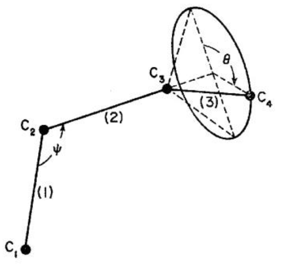
Figure 13.
Sketch of a covalent conformer (Figure 1.2 of [
10]), after Flory’s three-bond unit [
19].
Figure 13.
Sketch of a covalent conformer (Figure 1.2 of [
10]), after Flory’s three-bond unit [
19].
In our view, the free energy of the collection of chains assembled as a polymer is not equal to the scaled-up free energy of a macromolecule embedded in a mean field created by the influence of the other macromolecules; at least not below the temperature TLL (see below), which itself is a function of the dynamics of the experiment and the chain characteristics. In fact, for many experimental conditions, depending on temperature and other factors, our model of polymer interactions does not require, in its hypotheses and derivations, a description of the changes which occur to the individual macromolecules. The dynamic statistical systems dealt with, to determine the free energy and its structure (enthalpy and entropy), are not macromolecules in our approach. However, the fact that macromolecules compose the basic structure is essential, for instance to understand the basis of our new Dual-Phase statistics and to explain “entanglements,” for which our model provides a completely different interpretation than the ones offered by the conventional spaghetti bowl or tube models [
10]. A “covalent conformer” is not the same as a “free conformer” (
Figure 13), such as a small molecule used as the monomer in the polymerization process. Its interaction to other conformers by covalent bonding modifies the conformational potential energy of a free conformer, and this governs the statistical properties of a “free chain.” Here we are still “classical,” yet when dealing with a collection of chains put together, our approach differs from the classical one. Conformers belong to two types of sets: they belong to macromolecules, which link them via covalent forces, as we just said, and they belong to the grand ensemble of conformers which are linked by inter-intra molecular forces, van der Waals, dipole-dipole, and electrostatic interactions which affect and define the viscous medium. That duality is intrinsic to conformers, which we call the “dual-conformers” to mark this specificity. The potential energy of a dual-conformer is different from the potential energy of a conformer part of a free chain. To simplify, one could view the difference between our statistical model and the classical model to describe the properties of polymers as follows: according to the classical views, the statistical systems are the macromolecules, i. e., a network of chains; the properties of the chains are disturbed by the presence of other chains and by the external conditions (temperature, stress tensor, electric field, etc.). The classical definition of the statistical system contrasts with our approach whereby the statistical systems are the “dual-conformers,” not the macromolecules. The interactive coupling between the dual-conformers is defined by a new field of statistics, the Grain-Field Statistics, that explores the correlation between the local conformational property of the dual-conformers and their collective behavior as a dissipative network. In the following, for simplicity we will just call the dual-conformers “conformers.” Again to simplify, the statistics that are used by the classical models and our model to describe the rotational isomeric states (RISs) of the conformers are fundamentally different: the classical molecular dynamic statistics is the Boltzmann statistics, famous for its kinetic formulation of the properties of gases. The Dual-Split or Dual-Phase statistics, leading to the Grain-Field Statistics, is inspired by the classical Boltzmann concept but departs from it by defining a dissipative term in the equations and assuming that the free energy remains always equal to its minimum value, that of the equilibrium state, even for transient states. The kinetics created by such changes in the fundamental equations result in the formation of free energy structures, which we have once called “the energetic kinetic dissipative network of conformers (EKNET)” ([
20,
21,
22,
23,
24,
25]) and more recently, while dealing with rheology, “the elastic dissipative network” ([
10,
17]). In our analytical formulation of the dynamics of these “open dissipative systems of interactions” generated by our two modifications of the classical formula, we realized that essentially two mechanisms of structuration of the free energy prevail and compete: a “vertical structuring” and a “horizontal structuring,” each specifically applying its own version of the basic equations. This distinction increases the complexity of the analytical solution but is, in our opinion, a fundamental aspect of the way interactions work. The vertical structuring refers to a split of the units (collectively interacting in the system) into two compensating sub-systems having each a different statistical partition. The horizontal structuring offers a different split of the collective set, via the generation of Ns identical sub-systems, each with the same statistical partition. Each split mechanism generates a dissipative function. The total dissipative function ought to be minimized (it is 0 at stable equilibrium), a condition that creates their compensation, i. e., whether they work independently, in sequence, or together. The set of equations used to simulate the dynamics of a given dissipative system belongs to the general solution designated “the Grain-Field-Theory”. By applying these general principles to polymers, specifically, we can now summarize our model in one sentence: We define a polymer as a set of “dual-conformers,” i. e., a set of three-bond elements belonging or not to the same macromolecule, submitted to intra-inter molecular forces described by an energy potential to which the equations of the Grain-Field Statistics theory apply. In this review we only focus on the simplest simulation model, the vertical Dual-Split Kinetics. References [
18] and [
25] provide examples of more complex dynamic simulations that we suggest can be applied to simulate many specific problems of polymer physics, including the action of a mechanical stress field on the interactions between the dual-conformers network [
13]. In this paper, we present the Dual-Split Kinetics model in a way that makes its application to the TSD and TWD results more transparent. Working by analogy, one will recognize some identical patterns of behavior between the computer simulations and the real response of polymers using the TSD and TWD stimulation techniques. The simulation is presented in a shortened and simplified way to concentrate on the meaning of the concepts that could be useful to the study of interactive coupling in the amorphous state, the subject of this review. However, further details of the Dual-Split simulations (the effect of cooling/heating or annealing to simulate other viscous flow or thermal analysis results) can be found elsewhere ([
10,
11,
12,
13], [
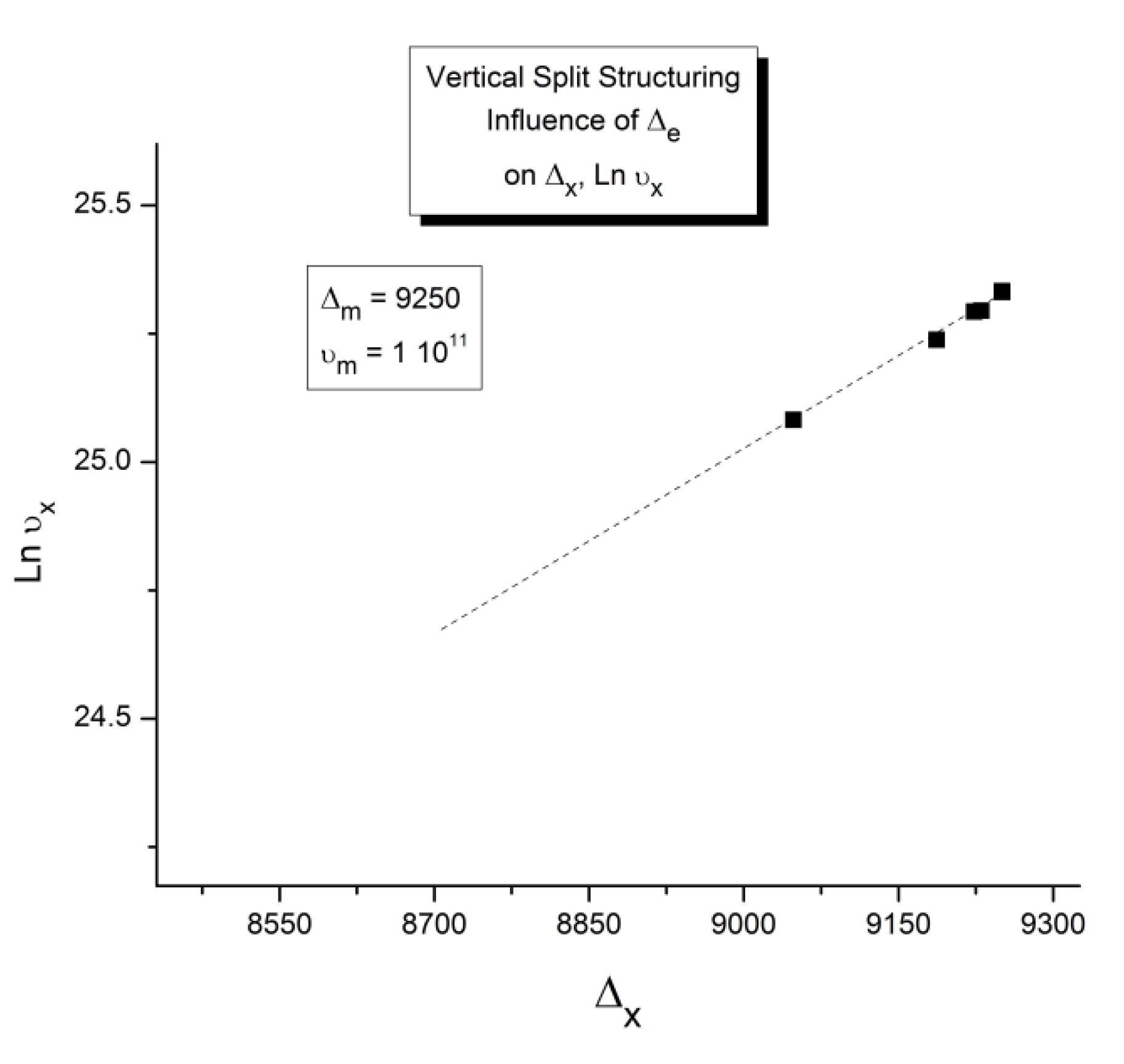
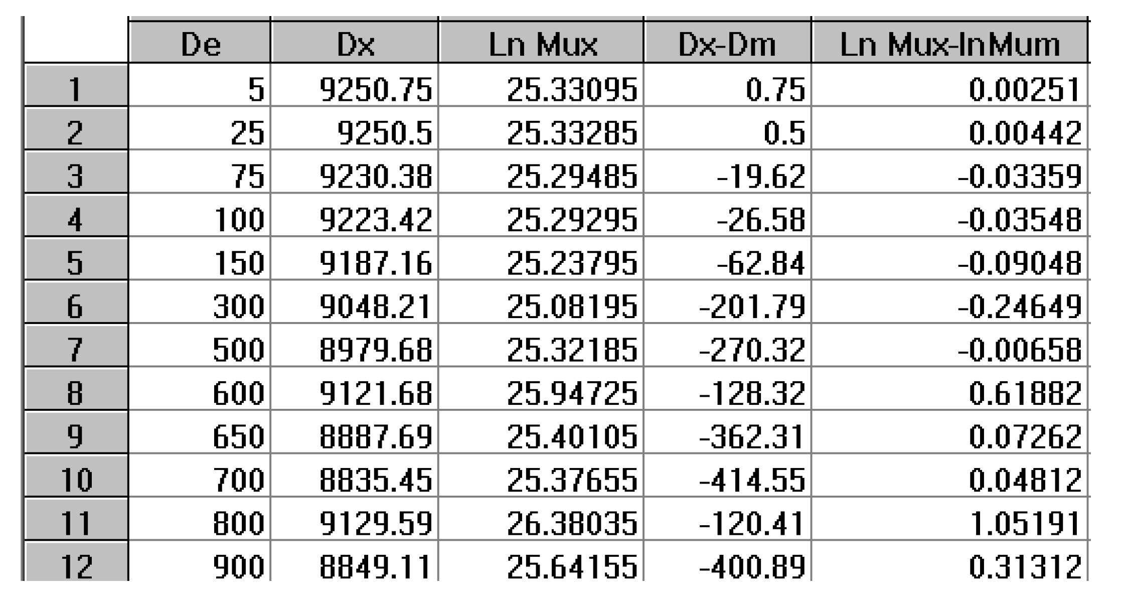
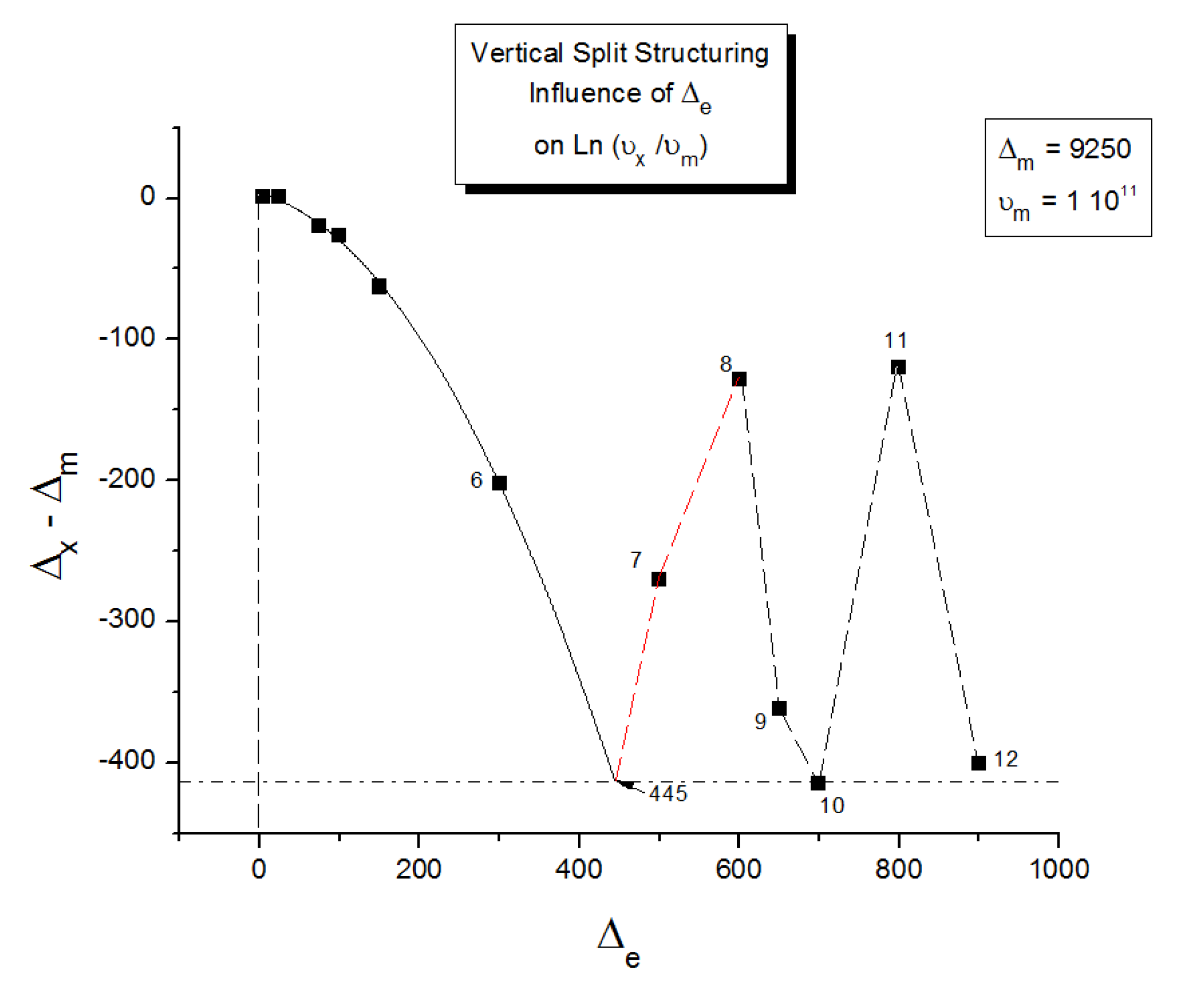
18]). As we will show below, the Dual-Split dynamics depend on the value of 3 fundamental parameters: υm and Δm which are independent of external actions such as a stress or a voltage, and Δe which can vary with the application of external actions. We limit ourselves, within the scope of this review, to dynamic situations that simulate simple experiments after the system initial conditions have been imposed; these simulations imply that the value of Δe has been pre-determined by the effect of an electrical or mechanical field applied prior to the dynamic thermal stimulation. We discuss in the DEVELOPMENT section how a thermal-electrical history procedure, such as the TWD characterization studied in this article, can be simulated by a modification of Δe with the temperature of polarization, Tp, and with the intensity of a voltage field. Once the value of Δe is set by these pre-conditions, the depolarization step of TWD can be simulated by a return to equilibrium induced b
y heating at constant rate in the equations of the Dual-Split Kinetics.
But first, let us describe the assumptions that led to the Split-Dual-Kinetics model, also called the EKTOR model (from the fusion of energetic and Kinetic considerations) or the EKNETICS equations since the result is the formation of a self-induced network, the dissipative network.
A2.1 Conventional Kinetics.
The study of kinetics is a discipline that describes the evolution of the units of a population of, say, chemical molecules, that participate in chemical reactions. Another example would be to describe the evolution of units of a population which could occupy different “states”. Many other terms have been used to describe the same objective: “statistics”, or “dynamics”, for instance, as shown in the following definitions: the population partition that evolves with time can be studied with the tools of “statistics”, a transient statistics in fact, a field also regarded as “dynamics”. All these definitions are used in our presentation. The important thing here is to define the terms quantitatively.
Consider a simple dynamic process such as a 1st order reversible kinetic equation between two states, t ↔ cg, controlled by an activated process with direct and reverse kinetic constants k1 and k2, with activation energy Δ1 and Δ2, respectively. One can write the following elementary set of kinetic and thermo-dynamic equations to describe the evolution of the system:
(1) Bo= (nt + ncg)
Bo= total number of units in state energy levels t, cg
(2) ΔG= RT* Ln(nt / ncg) is the Free energy of the system with
ΔGe= RT* Ln(nte/ncge) = RT* Ln (k2/k1) the equilibrium value
(the sub-index "e" corresponds to the equilibrium value). R is the gas constant.
(3) dnt/dt =-k1*nt + k2*(Bo- nt)
dncg/dt =-k2*ncg + k1*(Bo- ncg)
with:
k1 = υm exp(- Δ1/RT) and k2= υm exp(- Δ2/RT)
where υm is the Frequency Front Factor.
In the following, we call:
(4) Δe = (Δ1 - Δ2)/2 and Δm = (Δ1 + Δ2)/2.
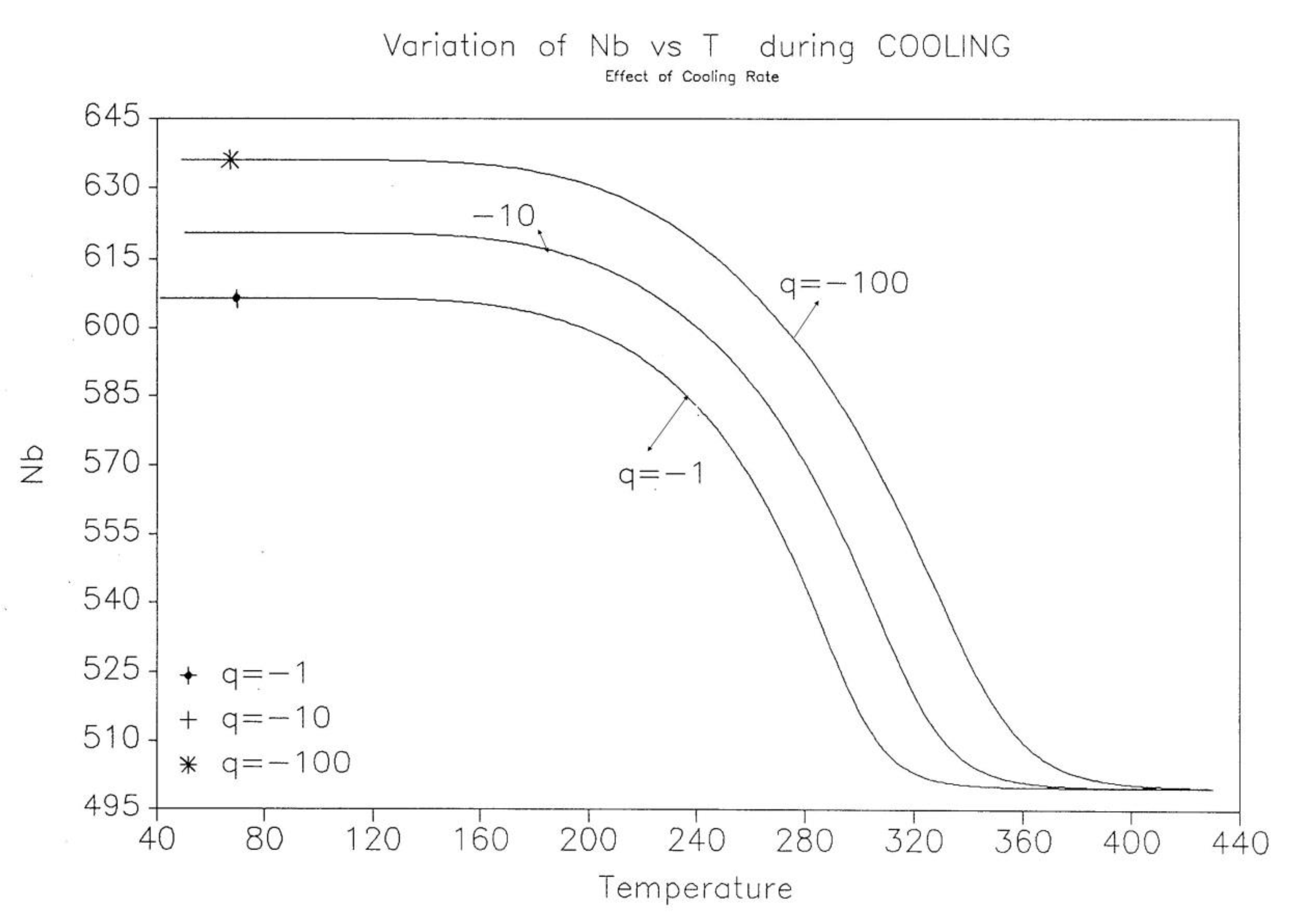
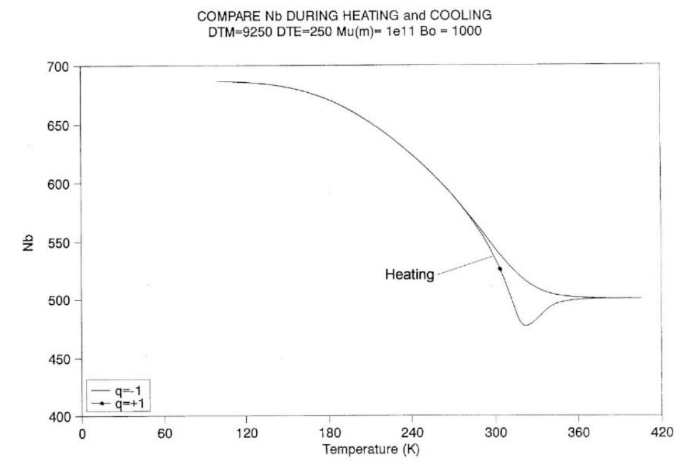
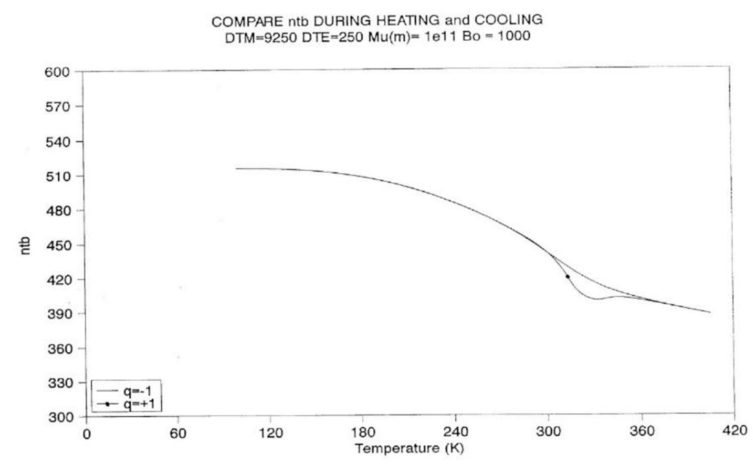
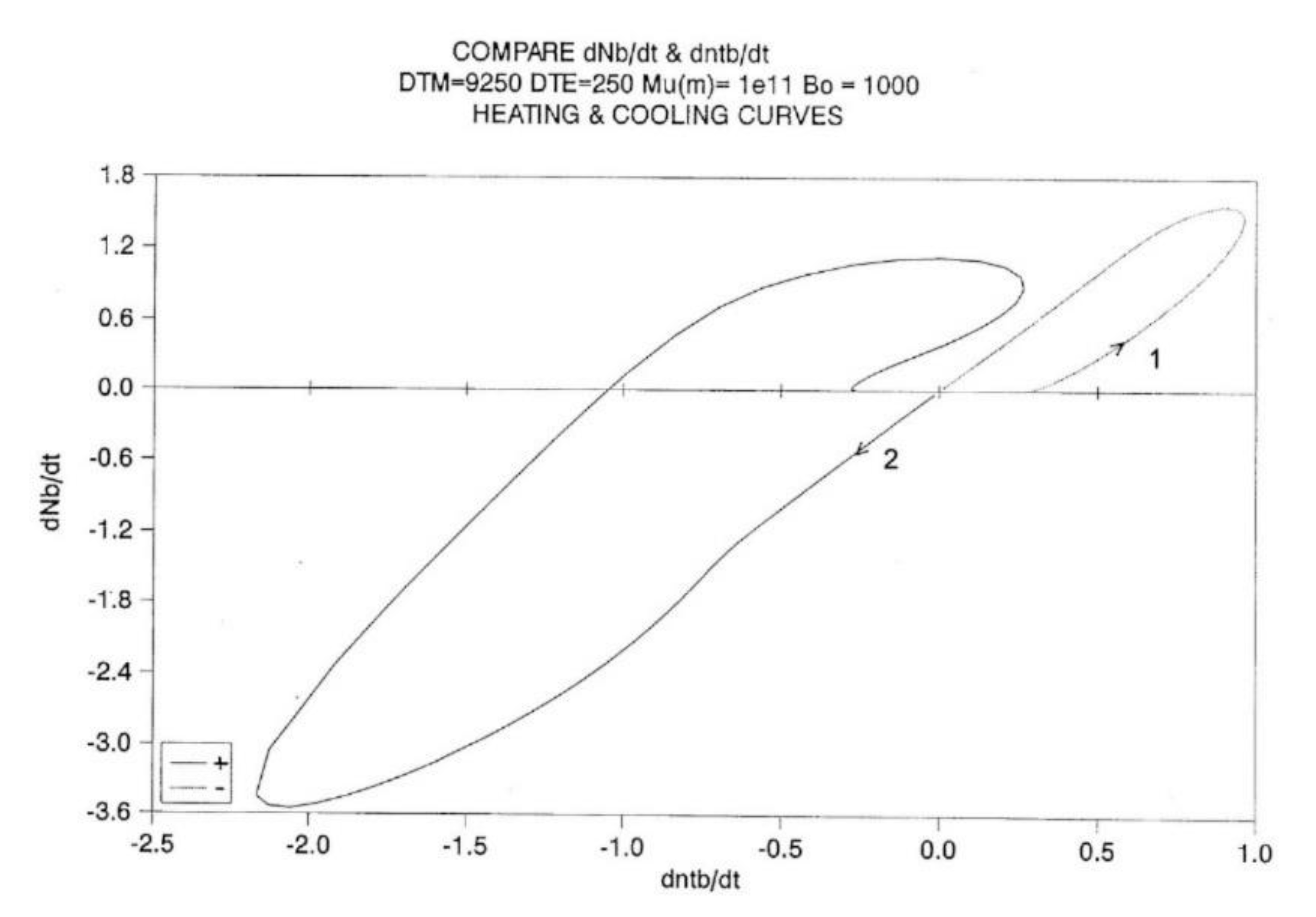
When the total number of units in the two levels, Bo, is constant, the statistics applies to a closed thermo-dynamic system. If the system is cooled at a constant cooling rate q = dT/dt, the now non-linear system of differential equations above can easily be solved (for instance, using a Runje-Kutta 5th order algorithm) to produce at each temperature a set of nt and ncg values, which can be compared to those of equilibrium at the same temperature. This will determine the effective departure from equilibrium due to non-isothermal cooling. Notice in the equation which gives the Free Energy that the term Ln(nt /ncg) reflects the departure of the Free Energy from its equilibrium value, and that nt, ncg are being determined by solving the kinetic set. Therefore, under non-isothermal conditions, the Free Energy plays a very subordinate role, and its magnitude is driven by the kinetic aspect.
For a classical set of kinetic equations it is clear that the transient Free Energy is not at its minimum value, since the value of the minimum Free Energy at any given temperature is known to be the equilibrium value at that temperature: ΔGe=RT*Ln(k2/k1).
When the system is brought out of equilibrium, and then allowed to relax, the kinetic equations drive the system back to the equilibrium state, which implies that the value of the equilibrium Free Energy is implicit in the formulation of the kinetic constants. In fact, the ratio of the two kinetic constants is equal to the thermo-dynamic constant, a quantity which gives the partition function for the two energy levels at equilibrium: ΔGe= RT* Ln(nte / ncge).
In conclusion, for classical kinetic equations under non-isothermal conditions, for which the solution is driven by kinetic considerations only, the Free Energy of the system is not equal to its minimum - equilibrium - value.
A2.2 Dual-Split Kinetics (EKNETICS).
Can we modify the set of equations driving the kinetics so the system Free Energy stays at its minimum value at all times? We call the solutions to this challenge “the EKNETICS equations”. The Dual Split Kinetics model, also called the EKTOR model, is the simplest EKNETICS set of rate equations fulfilling these conditions.
It is assumed that we can split each state cg and t into an F and b category, giving 4 states cgf, cgb, tf, tb; the result is a dual partition, between cg and t units on one hand, and between the f and b units on the other hand. The two partition functions are coupled.
In the following we present the assumptions driving the new EKNETICS and study the difference between its results and results obtained classically. The new equations converge to traditional kinetic equations at “long times”, which we will learn corresponds to either T > TLL, or under "true" equilibrium conditions. Under non-isothermal conditions the system becomes self-dissipative, i.e. ,for closed systems, that its free energy remains equal to its equilibrium value but its Eknetics cross-dual partition evolves in time.
A2.2.2 Dual-Split Kinetics (EKTOR EKNETICS)
Let's now consider the following modified system of equations, the “Vertical Dual-Split Statistics” system of equations, and comment on the assumptions made:
(6) Nb= ntb + ncgb
Nf= ntf + ncgf
Bo=(Nb + Nf)
(7) dntb/dt= (dNb/dt)/2 -k1*ntb + k2*(Nb - ntb)
dntf/dt= (dNf/dt)/2 -k1*ntf + k2*(Nf - ntf)
k1= m exp(- Δ1 /T)
k2= m exp(- Δ2 /T)
(the gas constant R is equated to 1 here and from now on)
(8) Ln (ntb/ncgb) + Ln (ntf/ncgf) + Ln (Nb/Nf) = 2 Ln (k2/k1) = 4Δe/T
q= dT/dt (under isothermal relaxation q = 0)
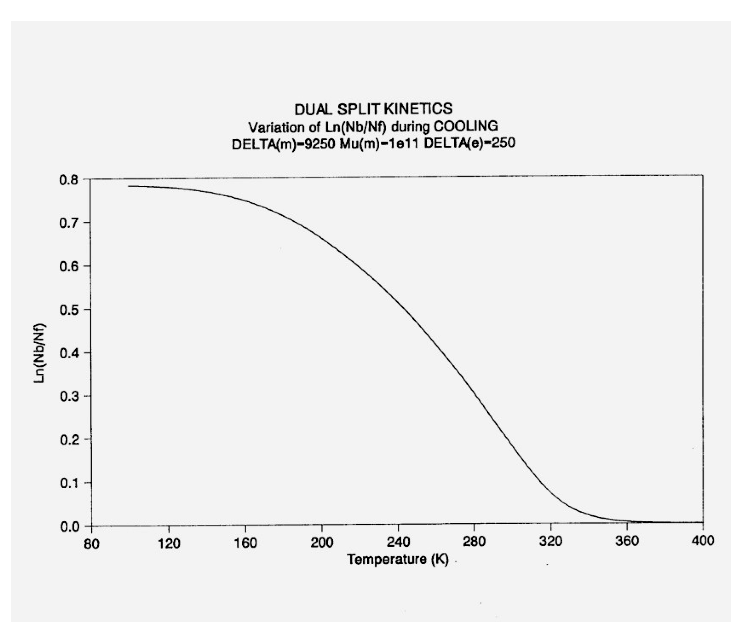
Note the presence of an additional term, Ln (Nb/Nf), in the expression of the Free Energy. This function is what we designate the "dissipative term". Its introduction is fundamental in our work on interactions; it is the source of the originality of the new statistics and results in the study of a new generation of dynamics open-self-dissipative systems. At equilibrium, Nbe=Nfe=(Bo/2) and therefore Ln(Nb/Nf) is equal to zero.
Also note, in Eq. (7), another important modification of the original kinetic equations, which now includes an extra term: (dNb/dt)/2 for the b-conformers and (dNf/dt)/2 for the F-conformers. The introduction of this term is to make the different rates consistent with the belonging of the units into one single closed system. Hence, the presence of this term is not an assumption: it is a requirement.
When Bo is constant in Eq. (7), i.e. for closed systems: (dNf/dt)/2 = - (dNb/dt)/2.
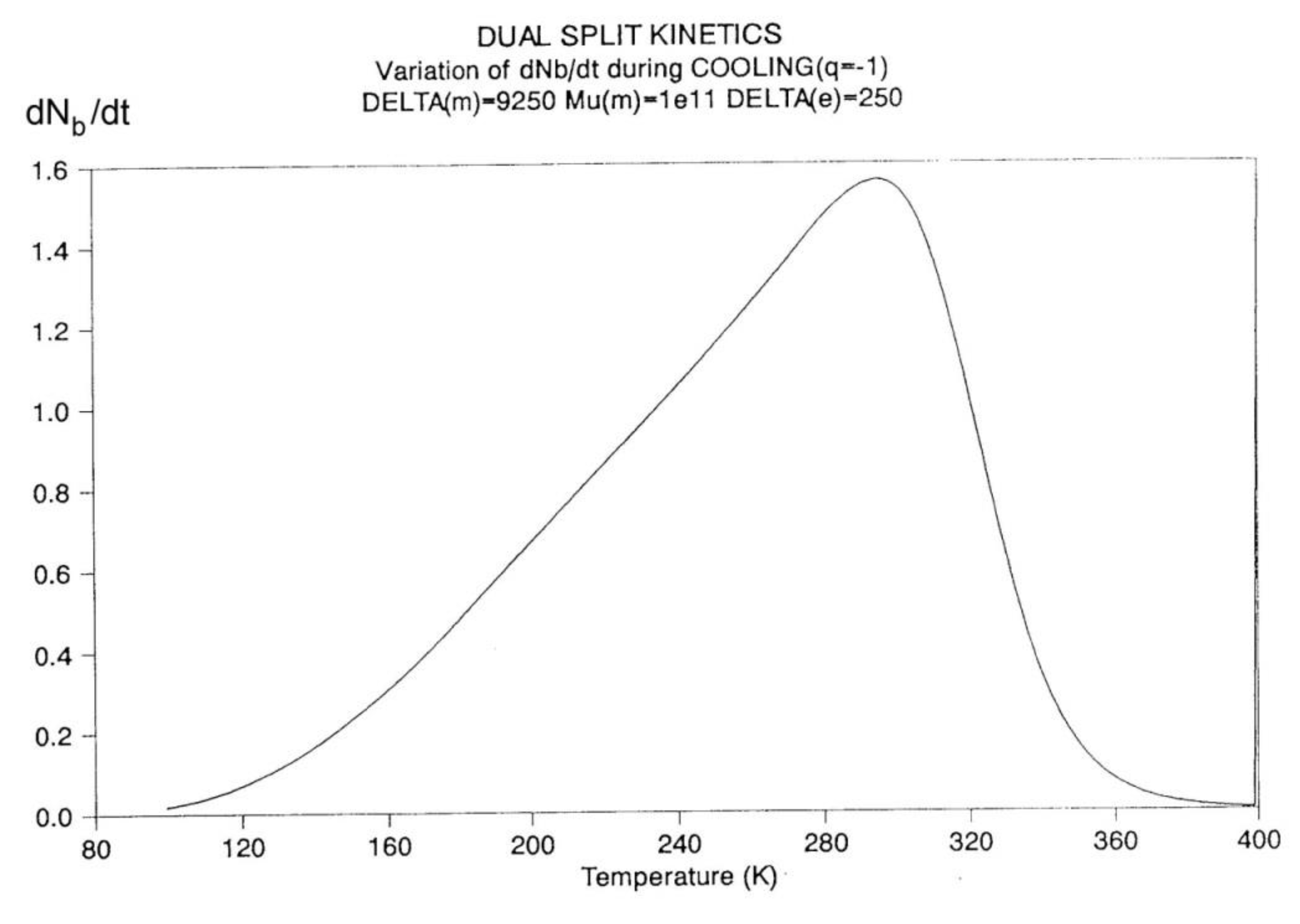
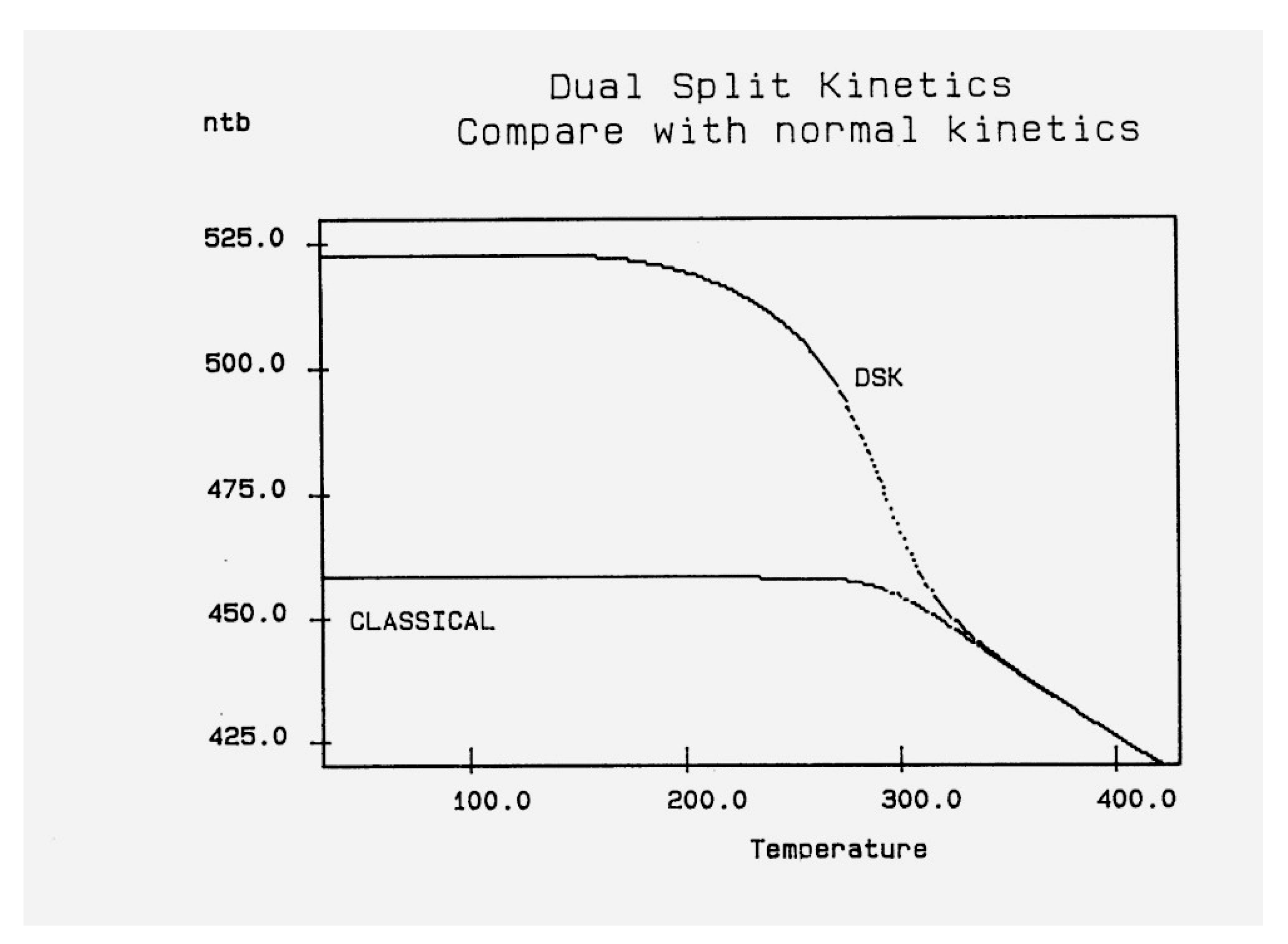
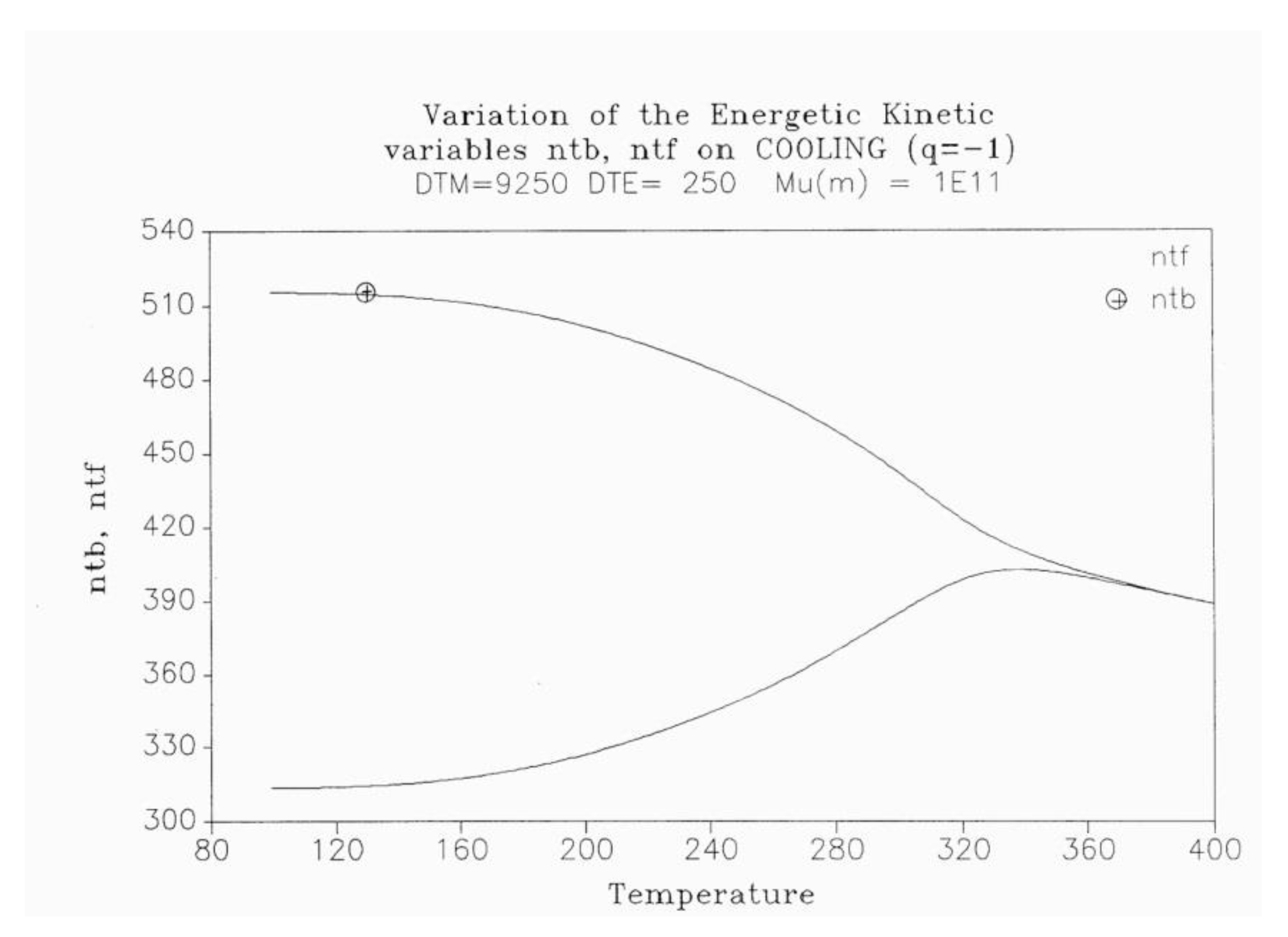
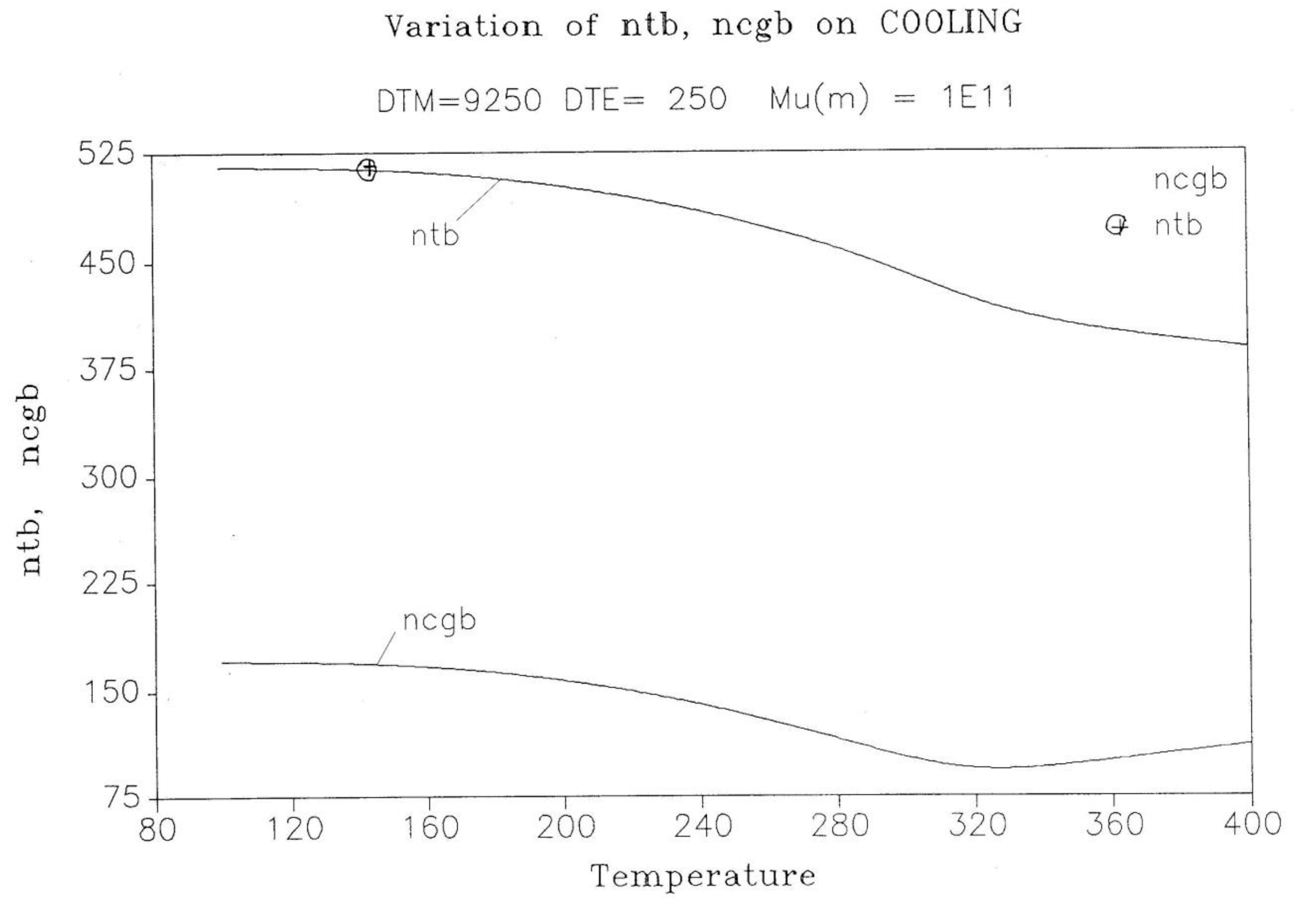
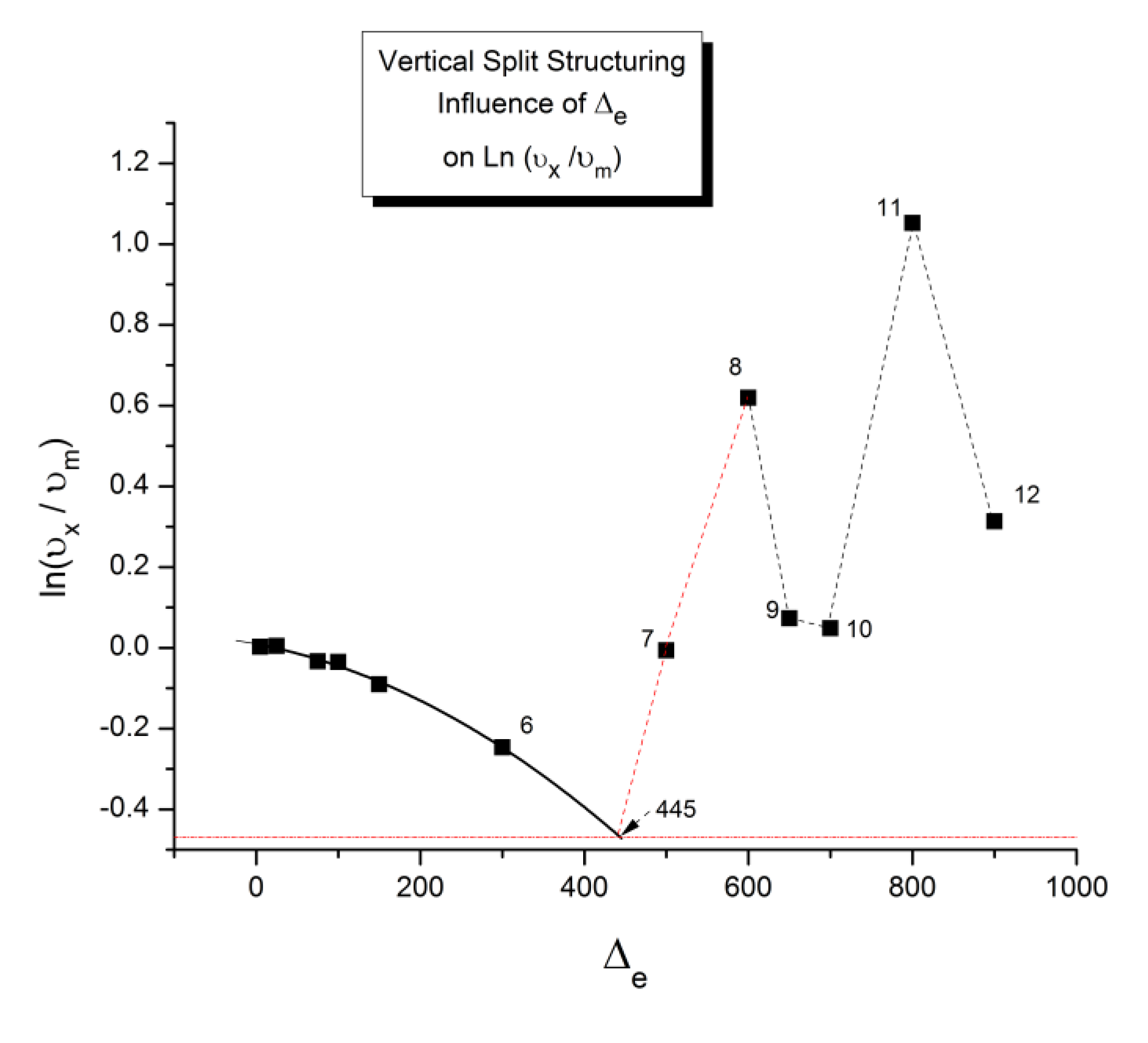
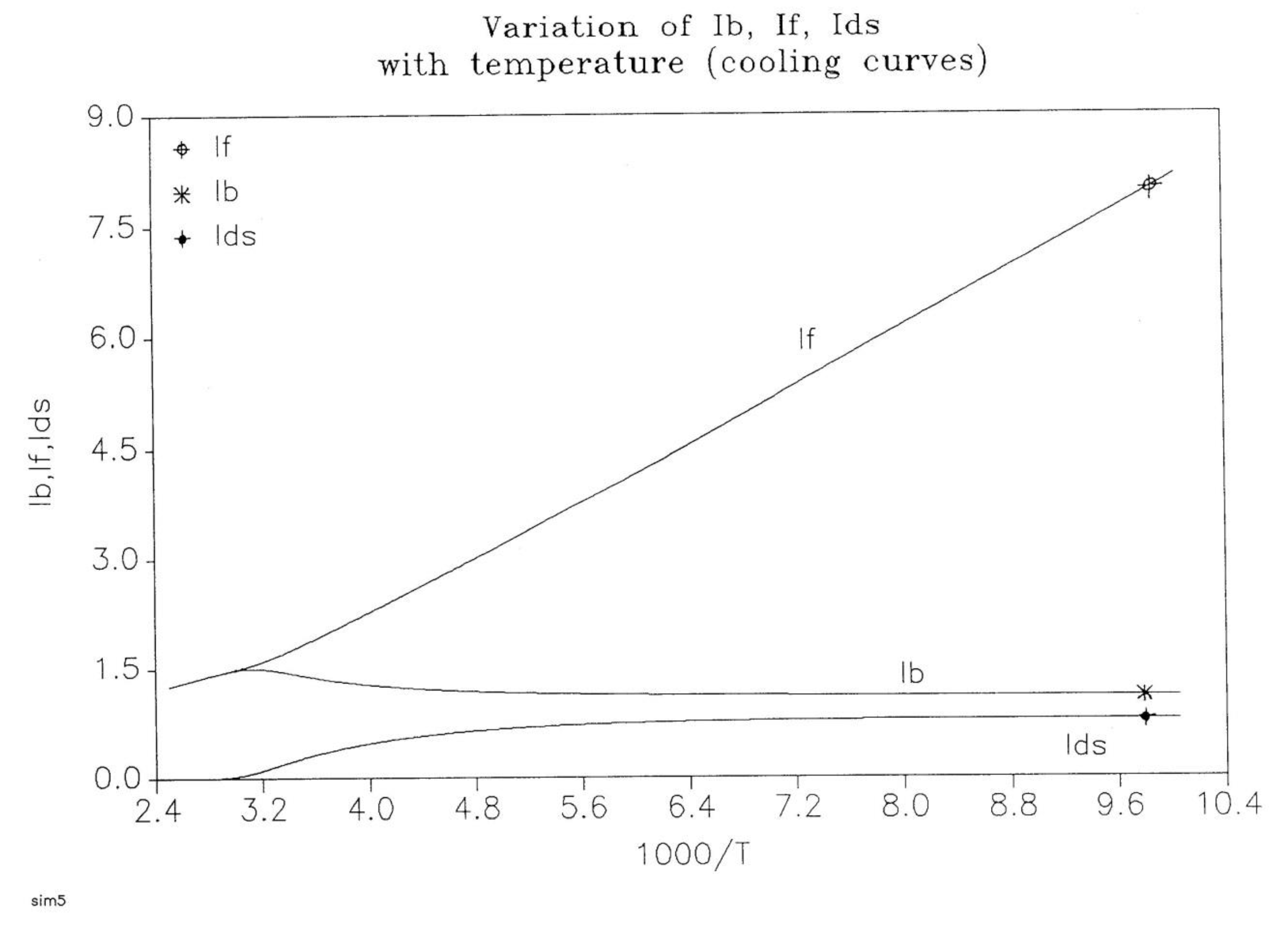
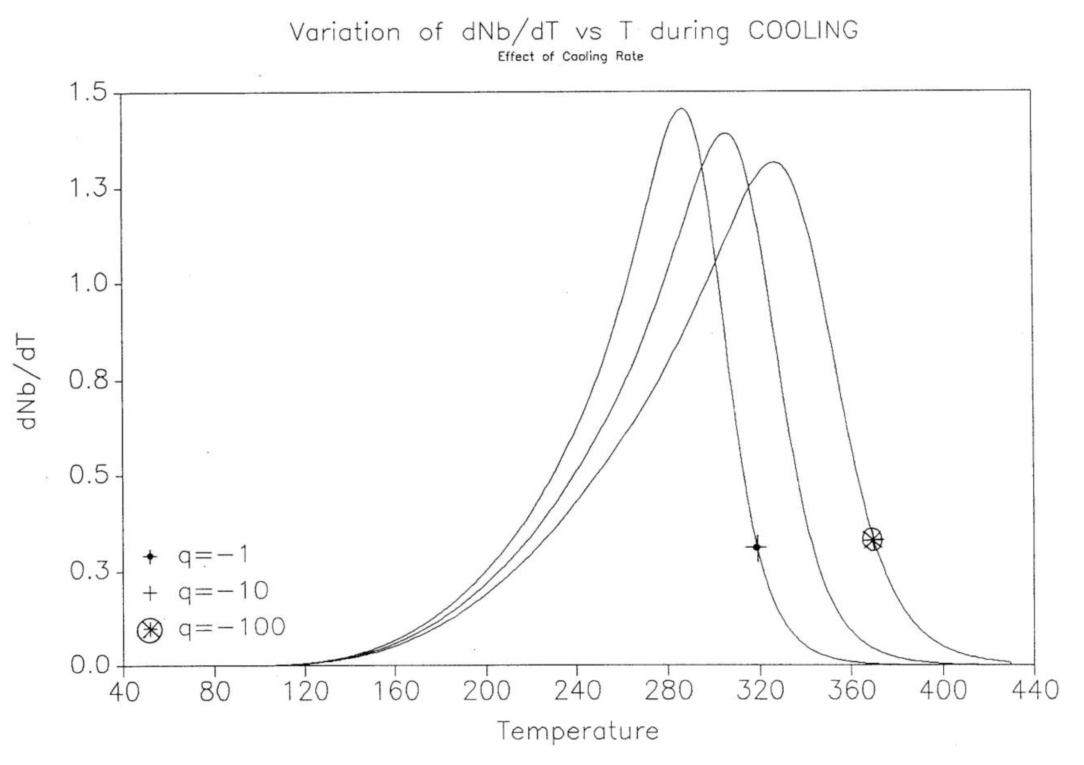
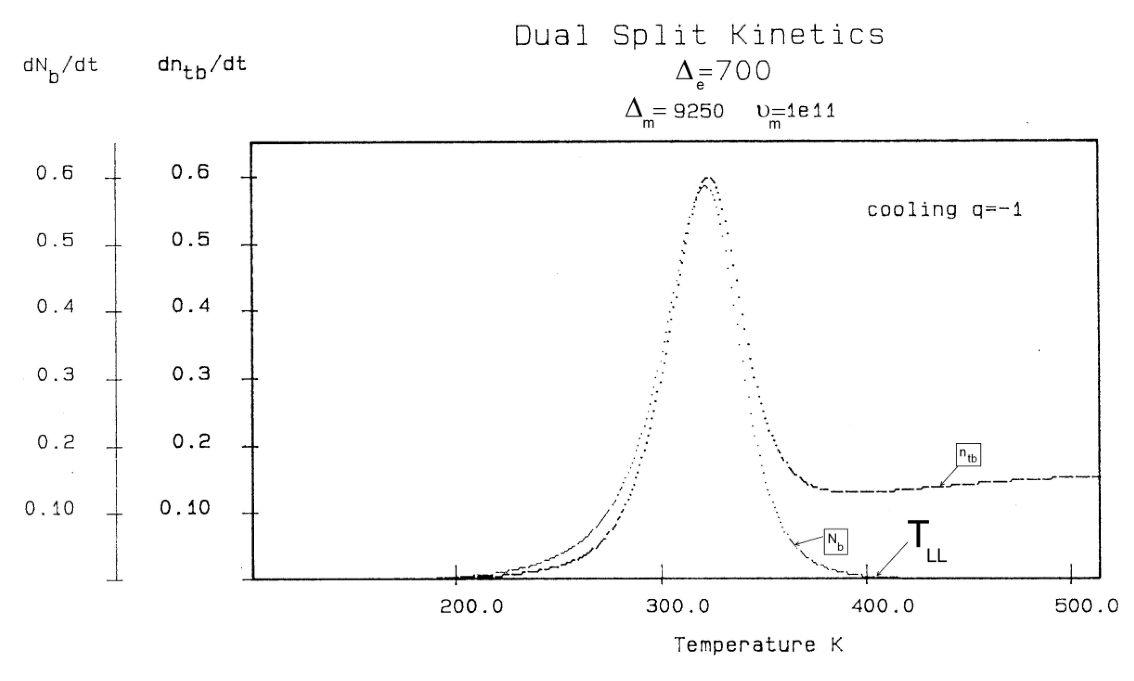
There is no assumption in Eqs. (6)-(8) regarding the variation of dNb/dt and its temperature dependence: the solutions come directly from Eqs. (6) to (8), as illustrated in
Figure 15, discussed in the next section. The coupling between energetic and kinetic constraints driving the new kinetic model is now apparent: the solutions for ntb, ncgb, ntf, ncgf, Nb are not obtained from a simple kinetic assumption (the expression of the kinetic constants and the proportionality between rate and population concentration). There is a real coupling between the free energy constraint and the kinetic constraints. The condition regarding energy is nothing other than a Minimal Principle, since it is assumed that the Free Energy remains that of the equilibrium state at the corresponding temperature. In conventional kinetics a system always evolves towards its minimum Free Energy, and therefore the minimum value is given by the equilibrium value. In the Dual-Split kinetics, the Free Energy remains equal to its equilibrium value when it evolves, which is a fundamental new assumption.
B2. The TSD MANIFESTATION OF Tg, the Tg,ρ PEAK and of TLL.
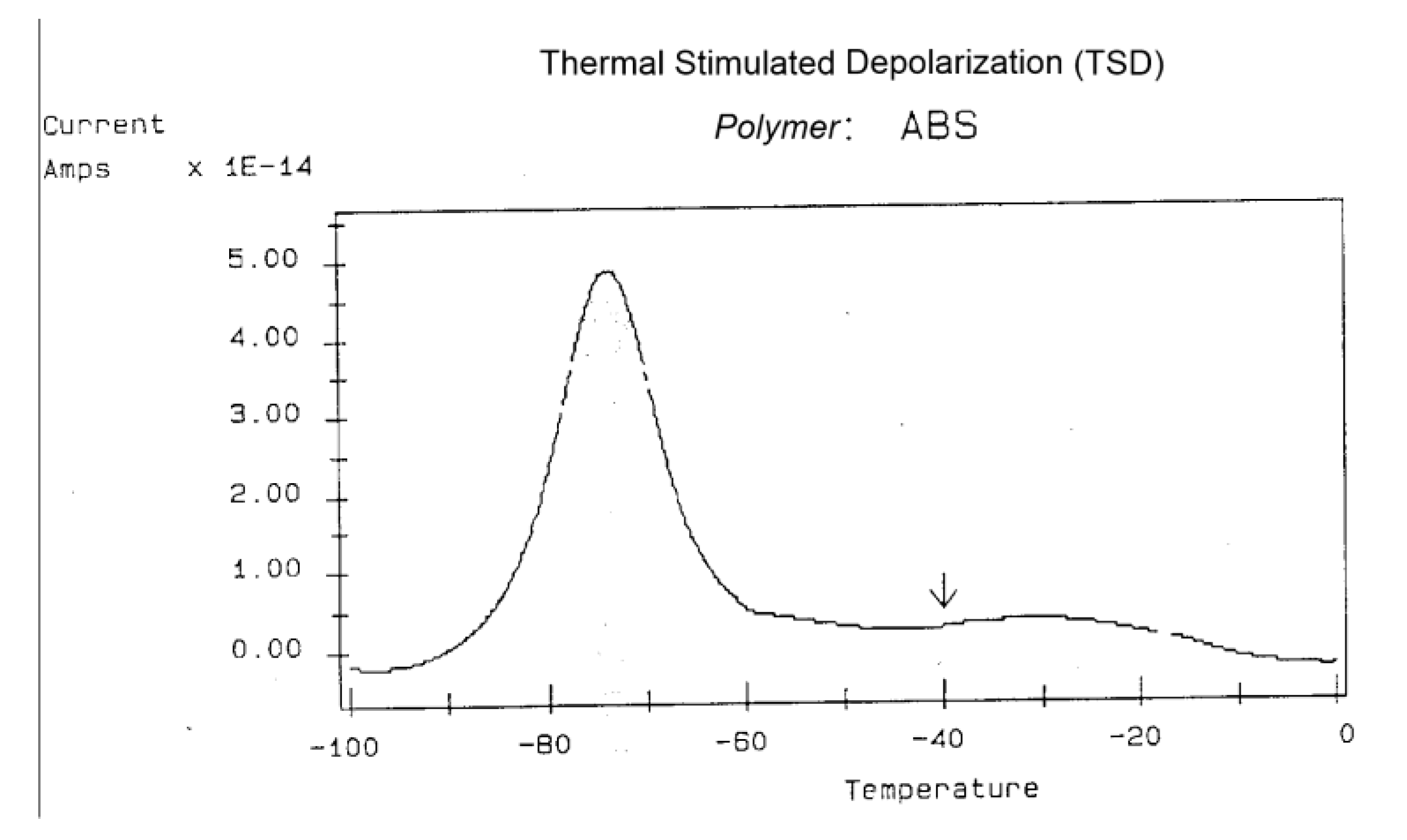
Some peaks of the TSD outputs are caused by the motion of the dipoles at characteristic transitions in the material, such as its Tg. Some other peaks are due to the interactions between the fundamental morphological structure of the amorphous phase (b-grains surrounded by F-conformers in the Dual-phase model ) and the electrical field, creating Wagner charges in F-micro-voids.
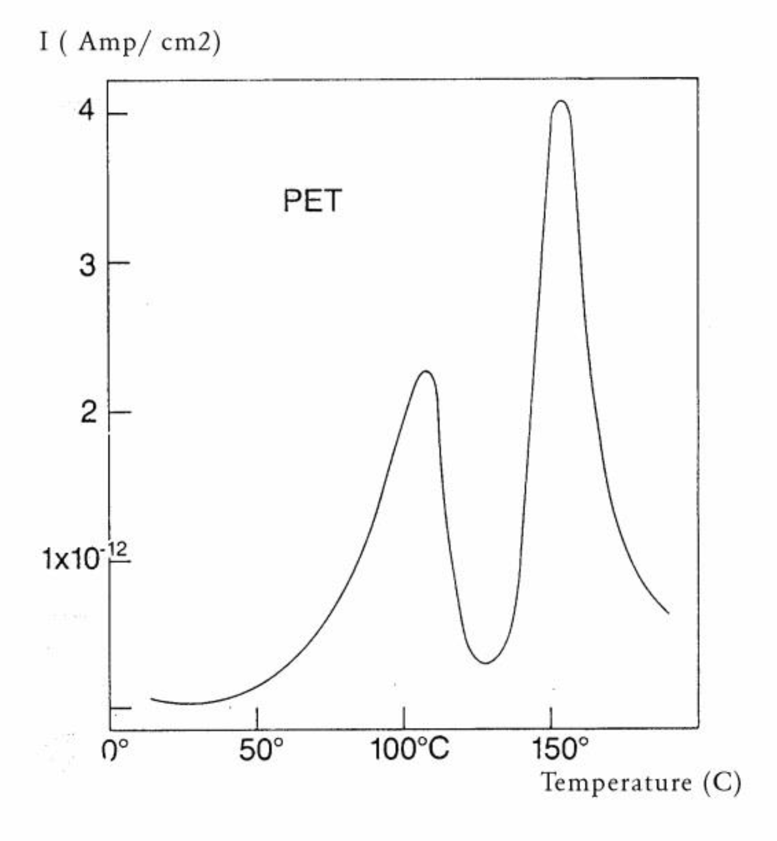
Figure 30 is a typical TSD curve for polyethylene terephthalate (PET). Two peaks are clearly visible, which we call Tg and Tg,ρ . The two peaks are separated by about 50 °C in this figure, and the intensity of the higher peak, Tg,ρ , is higher than the intensity of the first peak Tg.
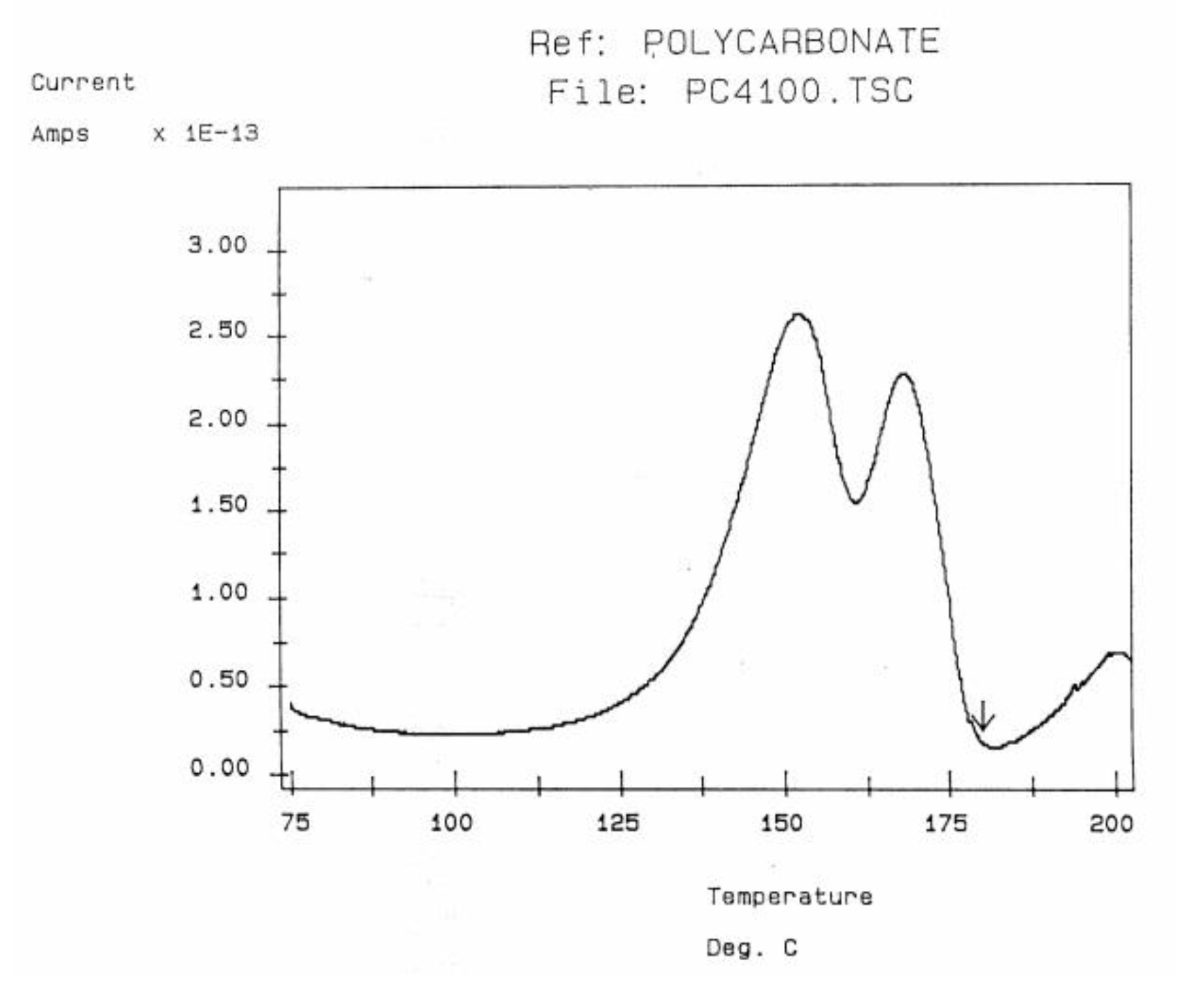
Figure 31 displays the TSD curve for polycarbonate (PC), showing Tg,ρ only 16 °C above the Tg peak.
Figure 30.
TSD depolarization curve obtained for PET showing the Tg and Tgρ peaks. The Tgρ manifestation can be correlated to the free volume content in the material.
Figure 30.
TSD depolarization curve obtained for PET showing the Tg and Tgρ peaks. The Tgρ manifestation can be correlated to the free volume content in the material.
Figure 31.
TSD depolarization curve obtained for PC showing the Tg and Tgρ peaks. The arrow indicates the temperature of polarization.
Figure 31.
TSD depolarization curve obtained for PC showing the Tg and Tgρ peaks. The arrow indicates the temperature of polarization.
The value of Tg,ρ observed by TSD is designated differently by various authors: Lacabanne and Boyer call that peak TLL [
28] and associate its existence with local order. Vanderschueren, Van Turnout and other authors call it Tρ [
2,
3,
29,
30] and speculate that it originates from the discharge of space charges delocalized in the structure. Extensive studies have shown that the relative intensity of the Tg and Tg,ρ peaks, as well as their respective position, depends on the thermal and mechanical history of the polymer, in particular physical aging. The magnitude of the Tg,ρ peak is also a function of the voltage field, increasing first and then leveling off as the voltage increases. The presence of the Tg,ρ peak is universal in the characterization of polymers by TSD. We find that peak just above Tg for all polymers tested: from paints to thermoplastics, from thermosets to rubbers, and for non-polar plastics as well as polar ones. This peak is apparently absent in the characterization of the same polymers by dynamic mechanical analysis (DMA) or DEA. It is stipulated here that differential scanning calorimetry (DSC) experiments can show Tg,ρ under special cooling and processing conditions which enhance its manifestation (see later). The position of Tg,ρ with respect to Tg depends, to a large extent, on the choice of the polarization temperature Tp , which enhances the respective magnitude and the resolution of the peaks by the effect of polarization selectivity mentioned in the previous section. Thus it is not uncommon to observe the Tg and Tg,ρ peaks merge into a broad intense peak for certain polarization temperatures, complicating their fine analysis. The transition TLL is also found by TSD, but it is located at a higher temperature, and it should not be confused with Tg,ρ . In some instances, the mechanical history of the specimen and the temperature of polarization are such that Tg,ρ and TLL merge or overlap, making the analysis even more complicated (
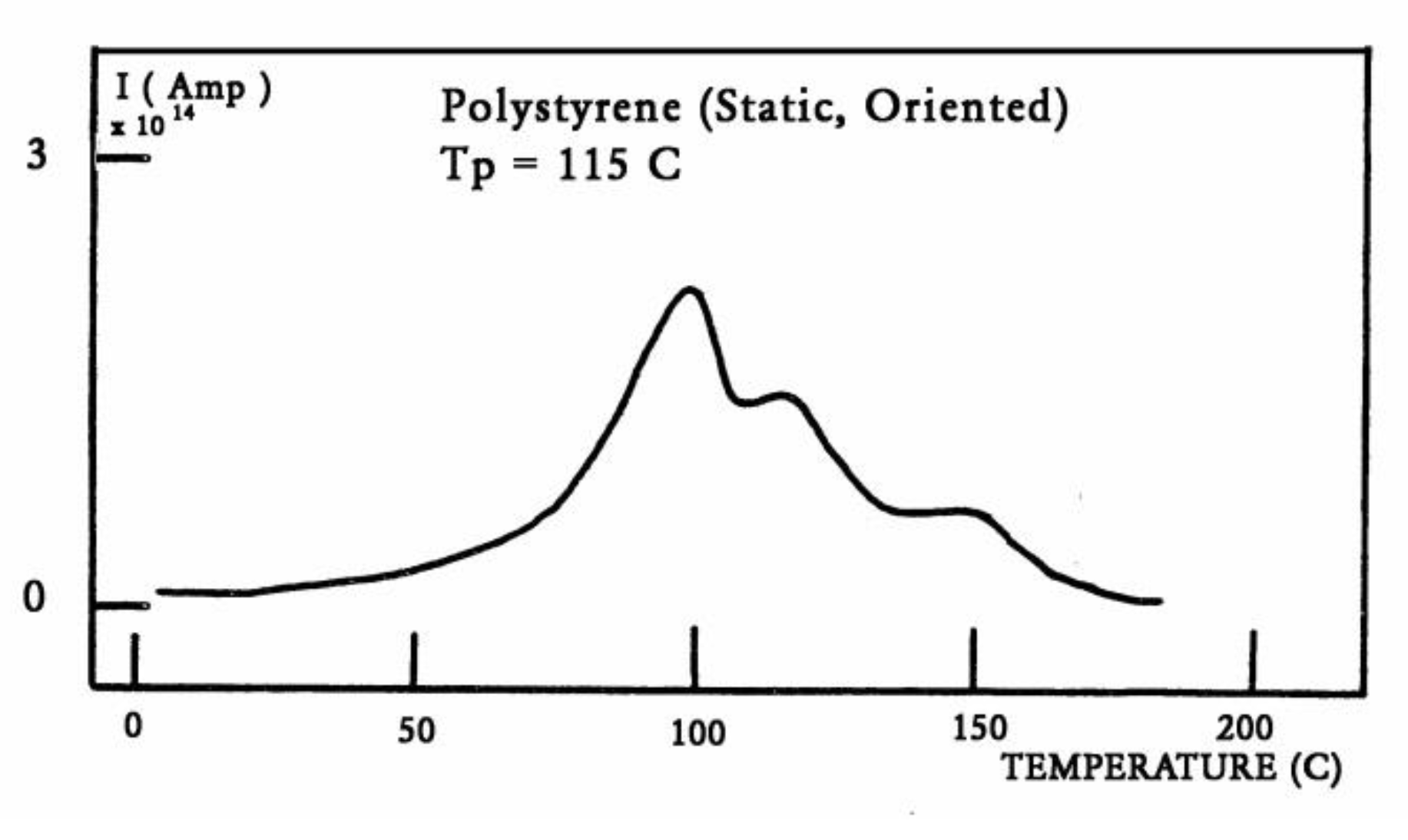
Figure 32). Fortunately, thermal-windowing normally allows a good separation of all the peaks, which can be isolated and deconvoluted individually. The only drawback with thermal-windowing at temperatures of polarization above Tg is that it modifies and partially erases the kinetic effects which are responsible for the relaxations under investigation. In other words, the manifestation of both TLL and Tg,ρ is favored by thermal history treatments which bring the specimen far out of equilibrium, but this is quickly erased by annealing above Tg , which occurs when the sample in the TSD cell is brought up to the polarization temperature. In
Figure 32, the specimen is a compression-molded 2-mm-thick polystyrene rapidly cooled to room temperature. A platen pressure of 226 bars is applied at 122 °C prior to and during cooling. The polarization temperature is 115 °C. Three peaks are clearly visible: Tg at 97 °C, Tg,ρ at 112 °C, and TLL at 150 °C.
Figure 32.
TSD depolarization curve obtained for an oriented compression-molded PS sample showing Tg and two other peaks above Tg .
Figure 32.
TSD depolarization curve obtained for an oriented compression-molded PS sample showing Tg and two other peaks above Tg .
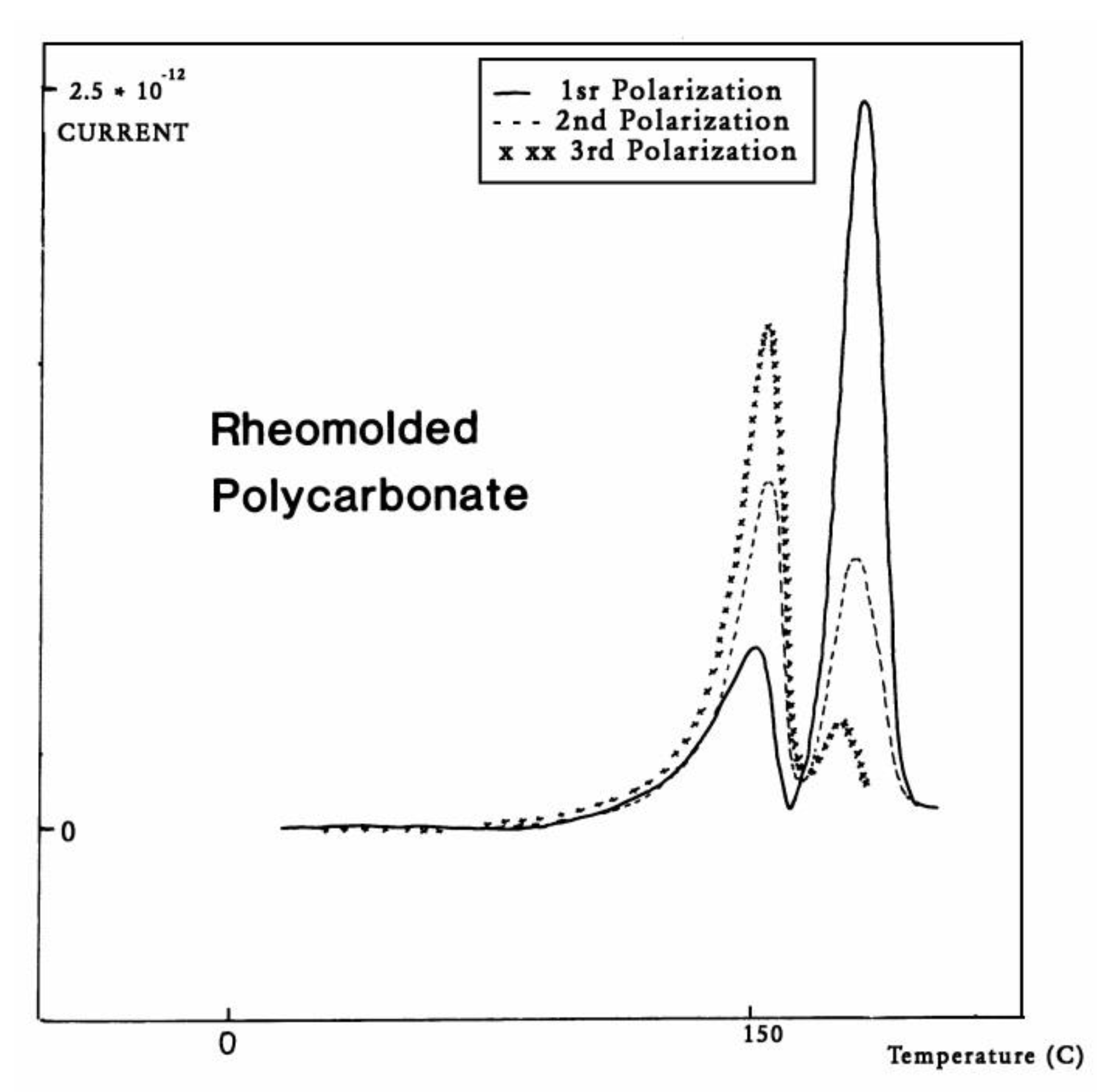
The intensity of the Tg,ρ peak is enhanced by fast cooling or any other thermo-mechanical process which creates a state of non-equilibrium in the polymer. The intensity of Tg,ρ decreases with annealing time, as is demonstrated in
Figure 33. In this figure, PC is subjected to a compression molding treatment involving a mechanical vibration as it is being cooled. This type of treatment is called Rheomolding and is described elsewhere [
8,
9]. In the TSD experiments shown in
Figure 33, a Rheomolded PC is rerun three times in a row without changing specimen. The same polarization conditions are used each time. Each run partially erases the initial thermal history of the specimen. We focus on the intensity and position of the Tg and Tg,ρ peaks. The first trace (first polarization) displays a very intense Tg,ρ peak relative to the Tg peak, but the intensity of this peak rapidly decreases for traces 2 and 3, as the initial state of PC returns to more traditional non-equilibrium conditions (cooling in the TSD cell, although rather fast, is no match to the severe cooling conditions imposed by Rheomolding). It is interesting to observe that as the intensity of Tg,ρ decreases, the intensity of the Tg peak increases, in a kind of complementary manner. The position of the Tg and Tg,ρ peaks also changes in a reverse way: as Tg maximum increases slightly, Tg,ρ decreases, giving the impression of fusion of the two peaks.
Figure 33.
TSD depolarization curve obtained for a mechanically pressurized and vibrated PC sample during its compression molding showing the compensation between the Tg and Tgρ peak intensity when the sample is annealed due to repeated polarizations done above Tg on the same sample.
Figure 33.
TSD depolarization curve obtained for a mechanically pressurized and vibrated PC sample during its compression molding showing the compensation between the Tg and Tgρ peak intensity when the sample is annealed due to repeated polarizations done above Tg on the same sample.
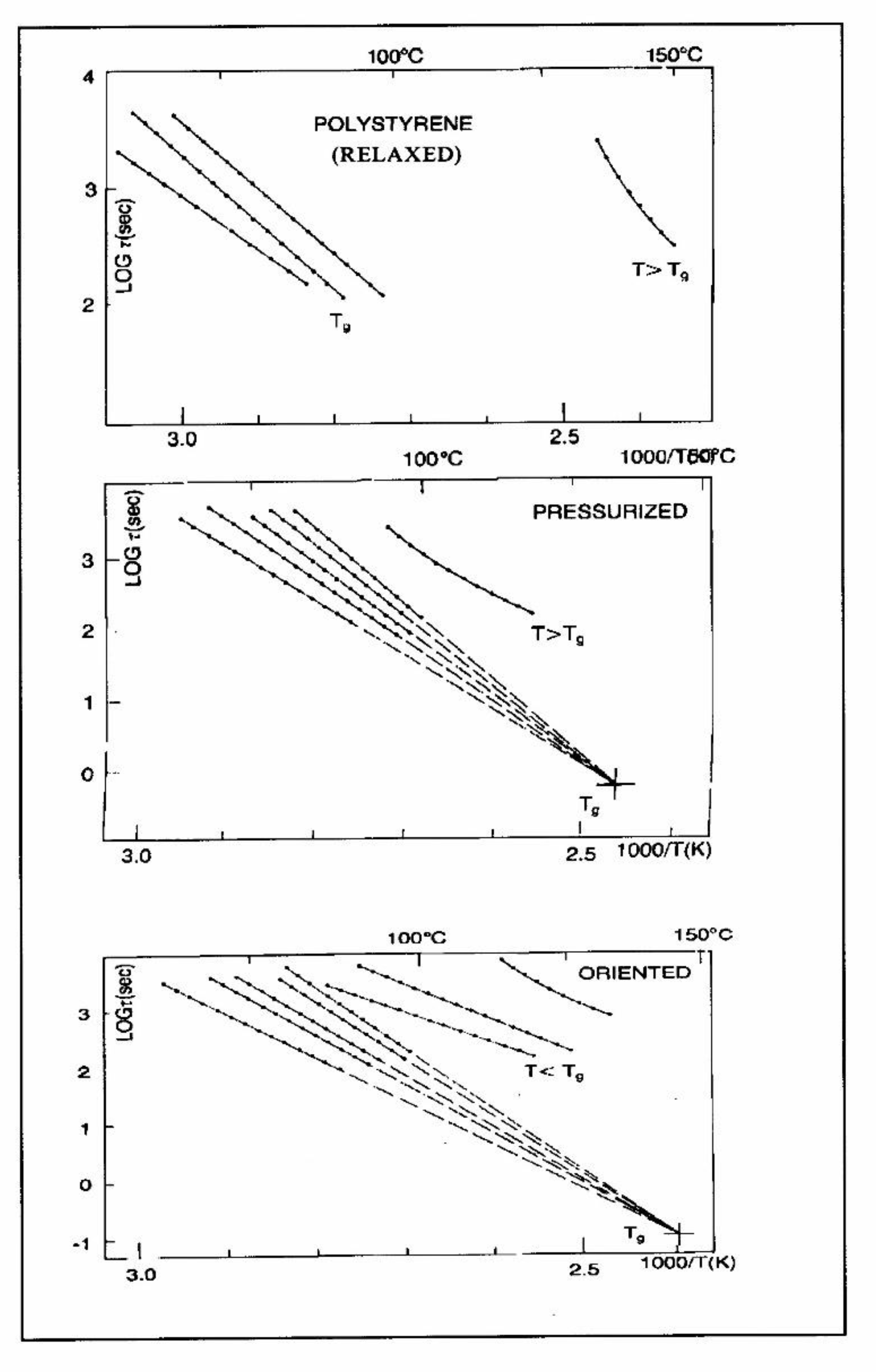
The understanding of the existence of Tg,ρ and TLL is offered in the Discussion (C1). As far as we are concerned, the Tg,ρ peak is real, big, often stronger than Tg , and located a few degrees after Tg . In this chapter, which deals with the applications of TSD, it is important to introduce the existence of peaks Tg , Tg,ρ , and TLL and suggest that their presence is universal in the context of the TSD characterization technique. It is not essential, however, to speculate about their origin. Let us just mention that Part I, Chapter 3 suggests a common kinetic origin to Tg , Tg,ρ , and TLL, and even to Tβ . The apparent complexity of the relaxation behavior arises for two reasons: even if Tg and Tg,ρ are kinetically related, their dielectric origin is different, because the effect of voltage field on the kinetic units responsible for their respective relaxation is different. In the case of Tg , the dipole moment relaxing is associated with a molecular dipole, but probably not so for Tg,ρ . The electric moment for Tg,ρ seems to be associated with ionic dipoles, or perhaps space charges. There is much evidence to confirm that the Tg,ρ peak is related to the “free volume” in the sample, which suggests that either local unstable ionic dipoles or space charges get trapped in the free volume of the polymer under the influence of the voltage field and relax at Tg,ρ . More details are provided in section C1 of the discussion where the “free volume” is defined in the morphology in terms of statistical units of the polymer chains. The difference between the characteristics of Tg,ρ and TLL is definitive: hydrostatic pressure lowers the value of Tg,ρ and increases the value of TLL. This is shown for Tg,ρ in
Figure 8 of the INTRODUCTION (A1). In this figure, polystyrene samples are prepared by compression molding under various conditions. In the top graph, a relaxed specimen is cooled under no mechanical stress at a very slow cooling rate. The Arrhenius transform of the Tg,ρ peak is shown at the extreme right of the graph; it is curved and can be fitted with a WLF type of equation, providing the free volume thermal expansion coefficient above Tg , and the temperature of infinite viscosity (the values found match well viscosity data). In the middle graph, corresponding to the “pressurized” specimen, the WLF curve is shifted towards a lower temperature. Another thermo-mechanical treatment is shown in the bottom graph.
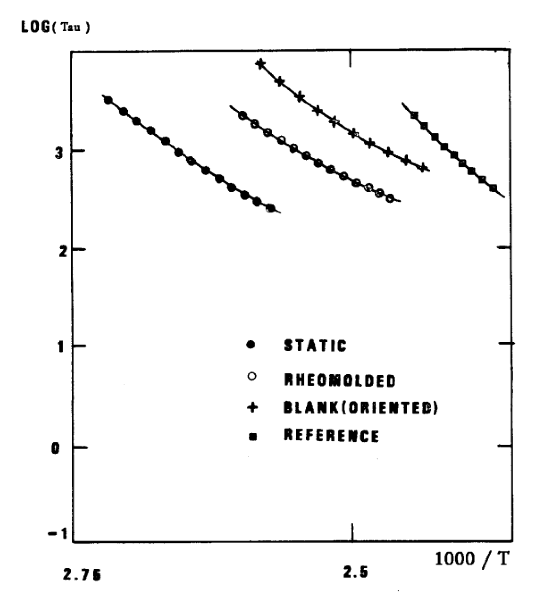
Figure 34 displays the Arrhenius transforms of the Tg,ρ peak for the several processing conditions: static pressure, Rheomolding treatment, oriented sample, and the relaxed polystyrene.
Figure 34.
Variation with the thermo-mechanical history of the molded PS of the Tgρ peak perceived as a WLF curve in the Arrhenius plane after conversion by the Bucci’s equation[
14,
15].
Figure 34.
Variation with the thermo-mechanical history of the molded PS of the Tgρ peak perceived as a WLF curve in the Arrhenius plane after conversion by the Bucci’s equation[
14,
15].
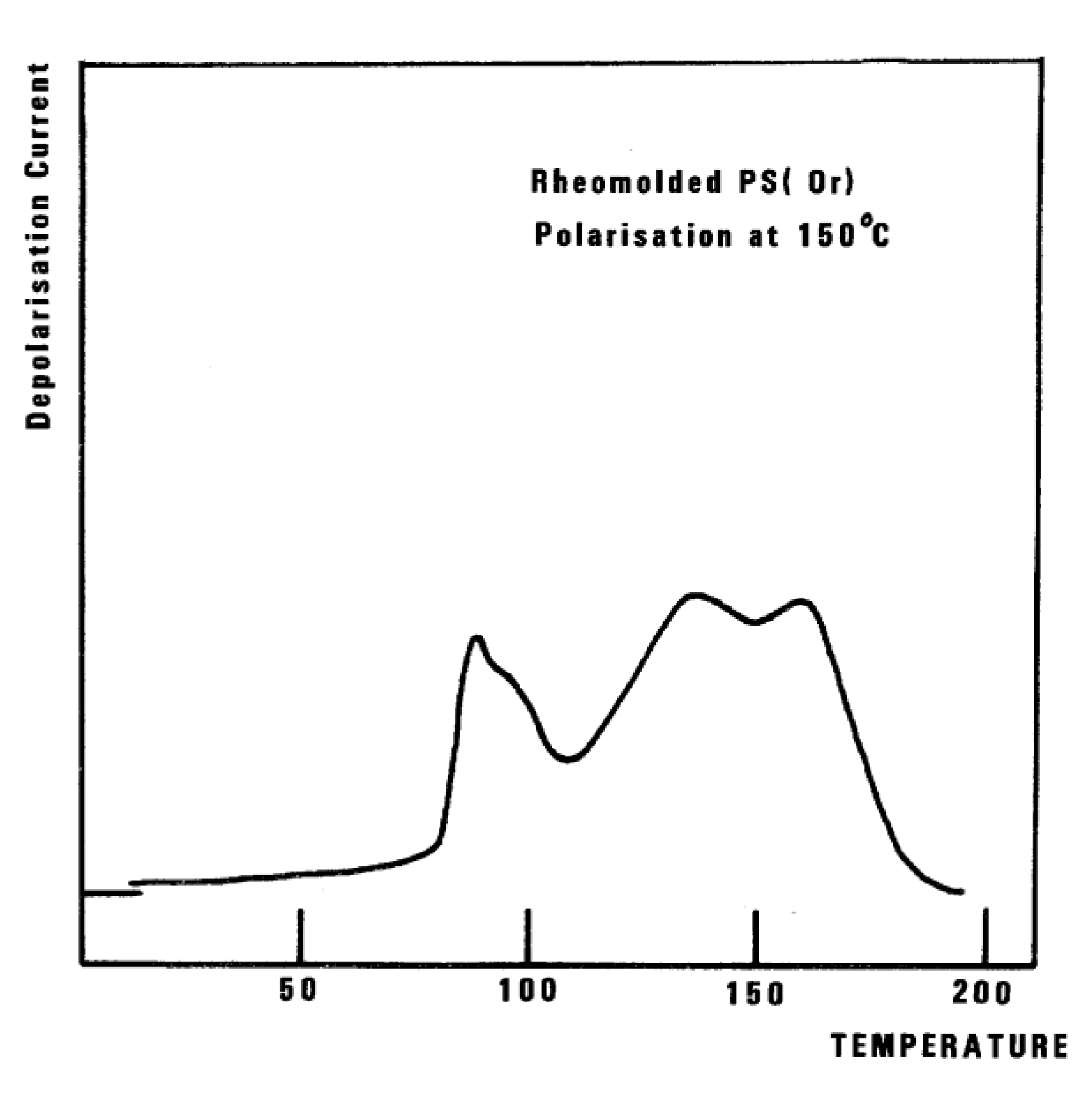
The relaxational mode obeys a free volume criterion for all conditions, but the content of free volume and the mobility at a given temperature, given by the horizontal position of the WLF curve, is a strong function of the state of polymer due to processing conditions. In some instances, the Tg,ρ peak is broad and contains a combined effect of molecular dipoles and free volume relaxations (
Figure 35). In such cases, thermal-windowing around the Tg,ρ peak produces several relaxation modes (
Figure 8, bottom curve), and sometimes one or two additional compensations are observed in the (T > Tg ) region up to TLL.
Figure 35.
TSD depolarization curve obtained for a vibrated oriented compression-molded PS sample (Rheomolded) after polarization at Tp = 160 °C showing Tg and two other peaks above Tg.
Figure 35.
TSD depolarization curve obtained for a vibrated oriented compression-molded PS sample (Rheomolded) after polarization at Tp = 160 °C showing Tg and two other peaks above Tg.
We consider TLL as the temperature, on heating, marking the end of a certain type of relaxation behavior due to cooperative kinetic interactions. Whether or not it actually corresponds to a TSD peak is irrelevant to our definition. For instance, we mentioned that TLL shows up in
Figure 32 as a peak at 150 °C. It might be more appropriate to categorize this peak as one of the kinetic manifestations resulting from the cooperative kinetic process already giving rise to Tβ , Tg , and Tg,ρ . It is suggested in Part I, Chapter 3 and in references [
25,
31,
32] that the mechanism of relaxation is due to the coherence between the collective behavior defining the statistical ensemble and the local existence of Dual-Phases (the b and F phases) which describes the interactive coupling between the conformers belonging to the macromolecules modulating both the sub-Tg and the (T > Tg ) kinetics. In that regard, TLL is probably more at 175 °C than 150 °C in
Figure 32, and the peak at 150 °C should be considered as a manifestation of the modulation by the network (collective) of b/F interactions occurring in the phase richer in free volume and responsible for the Tg,ρ relaxation manifestation. This point is further illustrated in
Figure 36.
Figure 36.
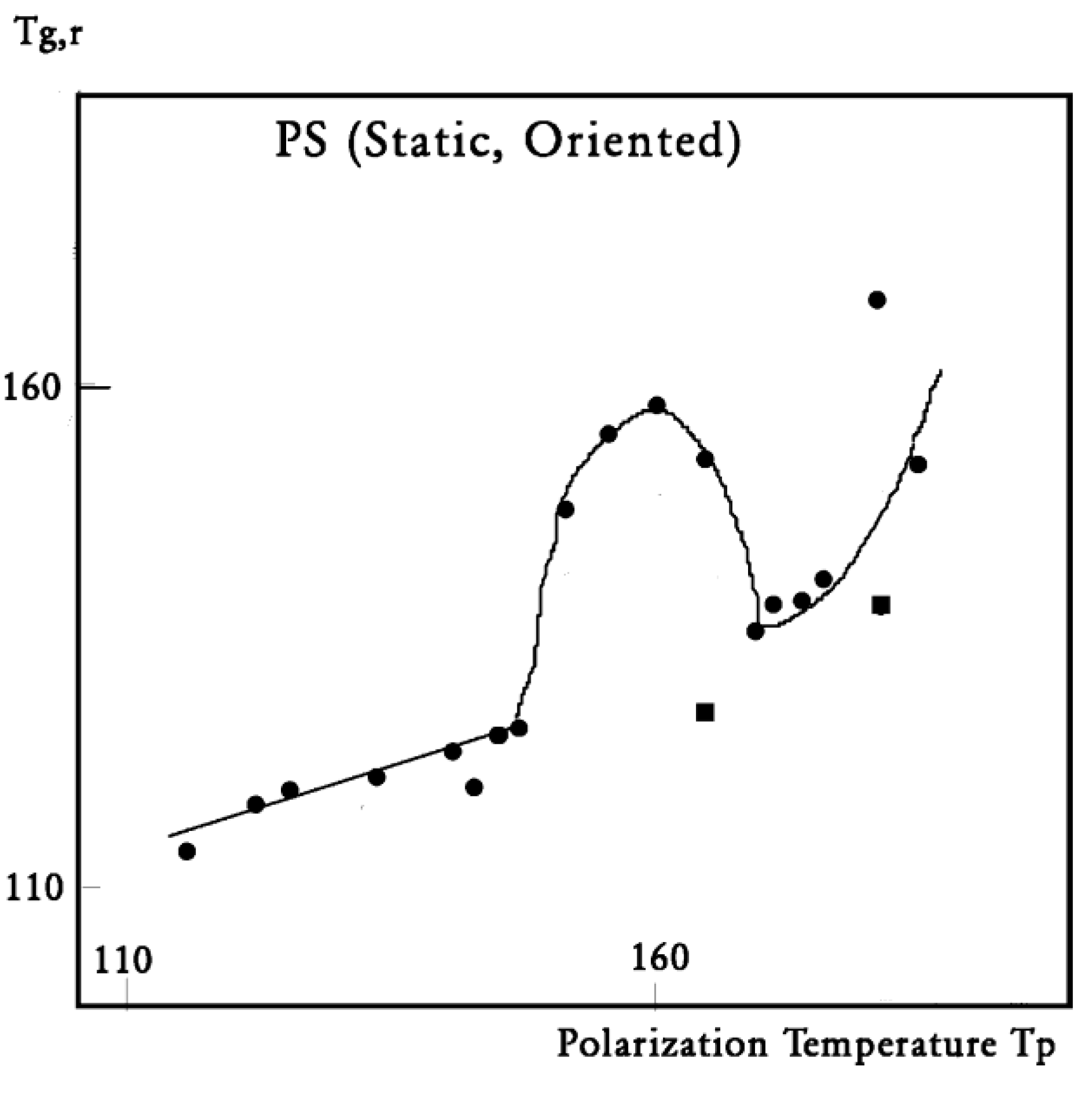
Variation of the position of the Tgρ peak with Tp for a static (no vibration) oriented compression-molded PS sample, exhibiting the TLL transition at 160 °C.
Figure 36.
Variation of the position of the Tgρ peak with Tp for a static (no vibration) oriented compression-molded PS sample, exhibiting the TLL transition at 160 °C.
In this figure, we plot the variation of Tg,ρ with Tp , Tg,ρ being considered the “first” peak observed above Tg . When a second peak appears, which we call T ′g,ρ , we indicate its temperature on this graph with square dots. One sees that Tg,ρ increases slowly and linearly with Tp (the slope is much less than 1), at least until Tp = 145 °C, a temperature at which Tg,ρ rises quickly to a maximum. The first split of Tg,ρ into two peaks occurs for Tp = 165 °C, and the second split occurs for 180 °C. In the case of a split, the temperatures of the two peaks are located on both sides of the “expected” Tg,ρ extrapolated from the lower values. The departure from the baseline at 145 °C reveals the kinetic presence of the network modulating collectively the interactions [
7]. Beyond Tp = 170 °C, the modulation by the elastic dissipative network of the inter-intra molecular interactions between the various dipoles is over. TLL would be 170 °C, according to our definition.
Figure 37.
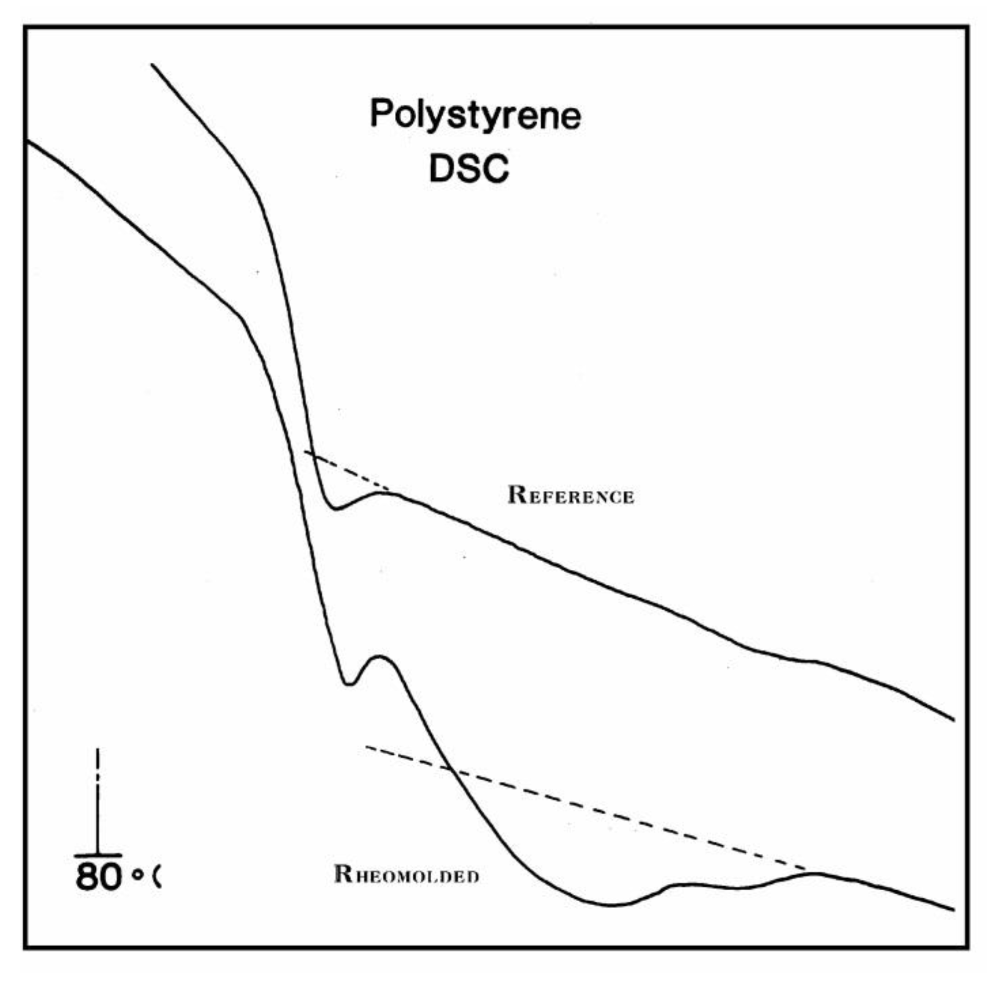
DSC trace comparison of two PS samples: the reference at the top is a compression-molded general-purpose PS. The bottom trace gives the response for a Rheomolded sample, compression-molded and vibrated at the same time while cooled. The cooling conditions were the same for both samples.
Figure 37.
DSC trace comparison of two PS samples: the reference at the top is a compression-molded general-purpose PS. The bottom trace gives the response for a Rheomolded sample, compression-molded and vibrated at the same time while cooled. The cooling conditions were the same for both samples.
The DSC trace for a Rheomolded polystyrene showing cooperative relaxation above Tg is compared in
Figure 37 with a reference trace (obtained by cooling the same sample in the DSC cell after the first run). The difference between the Heat Flow of the two curves is significant just above the Tg peak, and until the TLL temperature is reached. The thermal history of the Rheomolded sample, revealed during the first run, creates a thermal activity above Tg clearly similar to what is observed by TSD (
Figure 35). The thermal history is erased as the sample is heated in the DSC cell, and both reference and Rheomolded DSC traces are identical above TLL. We consider
Figure 37 as an important illustration by DSC of the existence of Tg,ρ and TLL. However, the sample preparation conditions imposed on the material, in order to reveal the thermal history, are quite severe in the case of a DSC technique. TSD, which works at a very low frequency equivalent (Part II, Ch.1 of [
5]), is capable of resolving the Tg /Tg,ρ kinetic presence with far higher resolution and sensitivity (note how thermal history of the Rheomolded PC of
Figure 33 is still revealed after the successive runs). The thermal analyst should be gratified: the Tg,ρ peak gives us a new parameter to characterize polymers. It varies with the processing conditions, and thus can be used to characterize the effect of processing variables (pressure, orientation, thermal history); it is often stronger than Tg and exists for non-polar materials when the free volume can be trapped with charges. It is perhaps the only peak which one can observe to characterize thick non-polar polymers. In that case, the “Tg ” found is possibly a Tg,ρ , several degrees higher than what would have been expected from a DSC comparison (the TSD Tg peak matches well the Tg obtained in a DSC experiment at a 20 °C/min heating rate).
B3. SUPER-COMPENSATIONS OBSERVED IN THE AMORPHOUS STATE OF SINGLE PHASE AMORPHOUS SAMPLES.
The objective is to explore the complexity of the phenomenon of compensation to better understand its origin. In the case of a multi-phase system, such as a segregated blend or a block copolymers, the relaxation map displays multi-compensations, each associated with the Tg of the corresponding phase. In the case of crystallizable polymers or liquid crystal polymers, multi-compensations are often visible both below and above the glass transition temperature of the polymer. All these apparent complexities are expected because of the presence of multiple phases in the material.
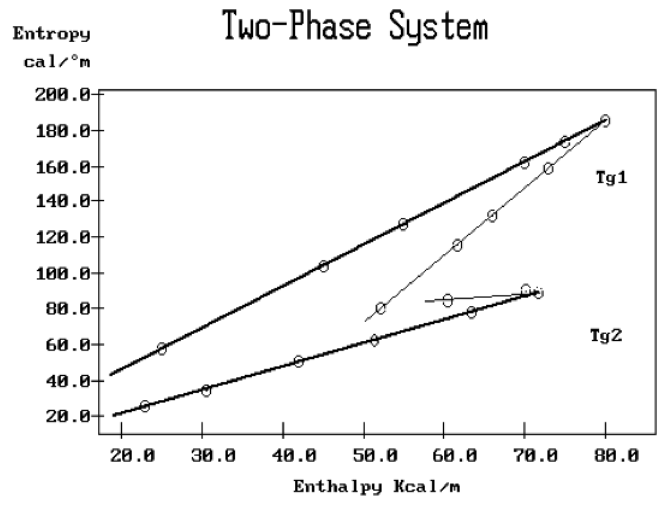
Figure 38 and
Figure 39 project what is respectively expected for the compensation search to look like for a two-phase amorphous polymer (blend or copolymer) or a single phase amorphous homopolymer such as polystyrene. In the case of a homopolymer (
Figure 39), only one Tg is observed. The compensation search leads to a single pair of compensation lines, one positive and one negative. The presence of two phases in the morphology is clearly revealed by two Tg s, and thus two pairs of compensation lines (
Figure 38). Comparison of the respective position of the compensation lines for the homopolymer and the block copolymer leads to a better understanding of the segregation characteristics between the phases and, in particular, of the degree of interpenetration and local compatibility [Part II, Ch.4 of [
5])). It is clear that in this case, there is a direct relationship between the number of compensation lines and the number of phases in the morphology.
Figure 38.
Schematic description of a compensation search in the EE plane to characterize the amorphous phases across their respective Tg for a two-phase system; typically for a block polymer.
Figure 38.
Schematic description of a compensation search in the EE plane to characterize the amorphous phases across their respective Tg for a two-phase system; typically for a block polymer.
Figure 39.
Schematic description of a compensation search in the EE plane to characterize the amorphous phase across Tg for a single-phase system; typically for an amorphous homopolymer.
Figure 39.
Schematic description of a compensation search in the EE plane to characterize the amorphous phase across Tg for a single-phase system; typically for an amorphous homopolymer.
It will be shown in this section (e.g.
Figure 55) that for a true monophasic amorphous polymer, in this case Polystyrene, not only is it possible to observe several compensations but also to vary the number of compensations depending on the thermomechanical history: the processing variables, the cooling rate, the amount of pressure, vibration, orientation, etc. This unexpected complex behavior has remained controversial: Lacabanne and Bernes [
35] have suggested that the several compensation points observed for polystyrene (and polycarbonate) were due to the presence of several amorphous phases, the indication of “local ordering,”. Furthermore, these authors suggested that TLL was the melting transition of these local micro-ordered structures [
39,
40,
41,
42]. In this section B3 we describe the multi-compensations in monophasic amorphous systems giving rise to super-compensations and propose in D3 an alternative explanation for the existence of super-compensations and of TLL based on the Dual-Phase model of the dissipative interactions.
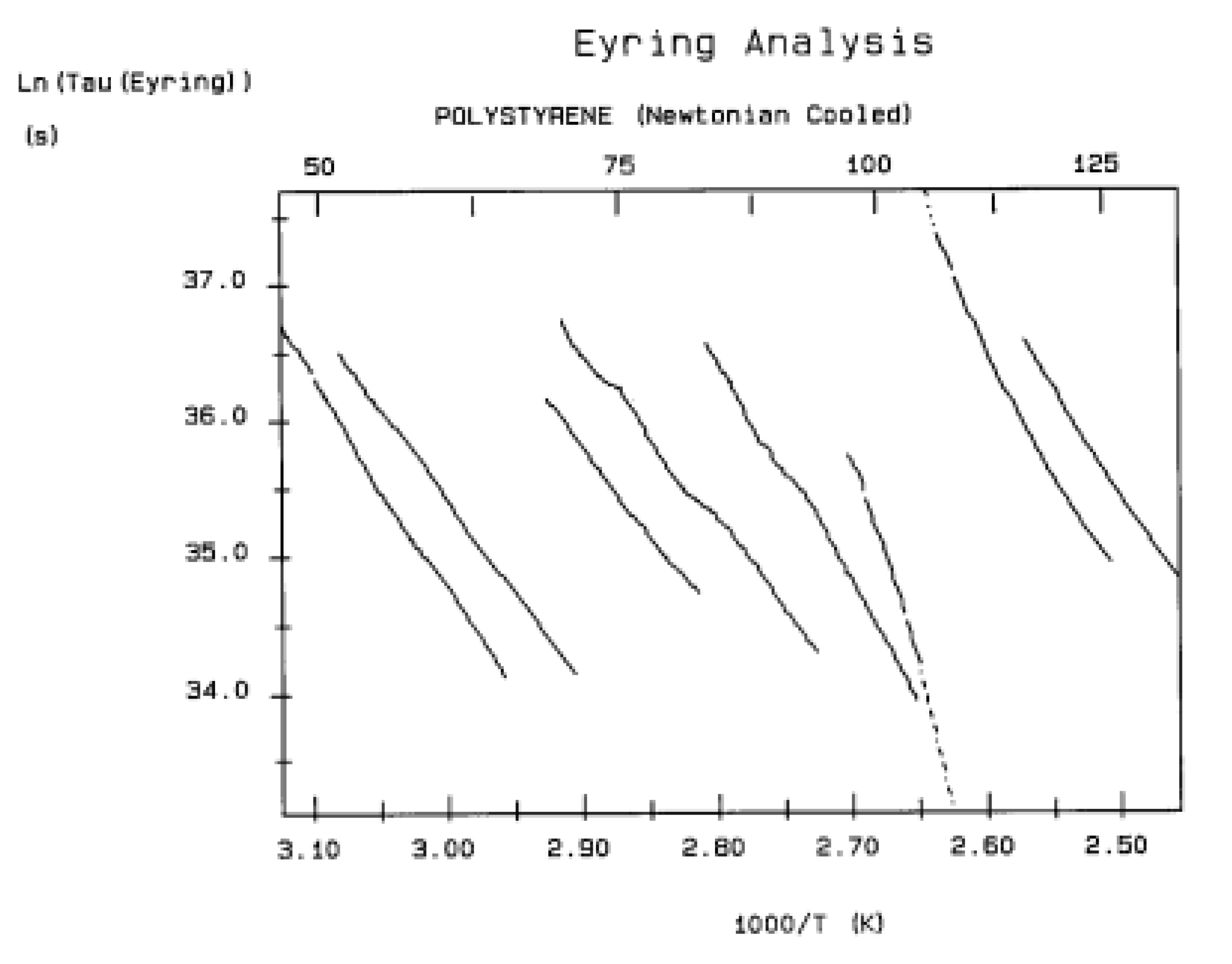
Figure 40 is a relaxation map in the “Eyring plane” (defined in A1) for a polystyrene disk (Tg ~ 100
oC). very slowly cooled from 180 °C to 50
oC in a platen pressure mold with virtually no pressure applied on the specimen during the cooling stage. The mold is cooled very slowly by “Newtonian cooling “, i.e.by shutting off the power to the heater cartridges after thermal equilibrium is reached at 180
oC and letting it cool by itself, without the use of cooling fluids in the cooling channels of the mold halves. This procedure resulted in a very slow cooling: it took approximately 7 hours to cool the mold down to 50 °C.
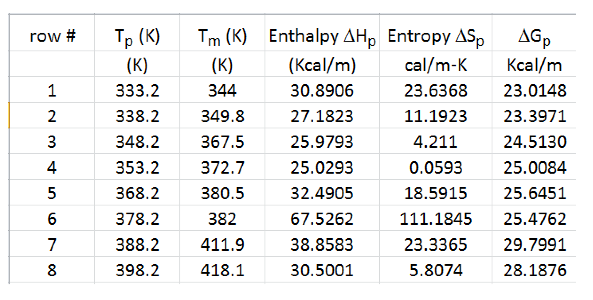
Table 1 gives the thermos-kinetic parameters as a function of Tp: ΔHp(“enthalpy”), ΔSp(“entropy”) and ΔGp(“Gibbs”), as well as the value of the polarizing temperature, Tp, and of Tm, the temperature at the maximum of the Debye depolarization peak.
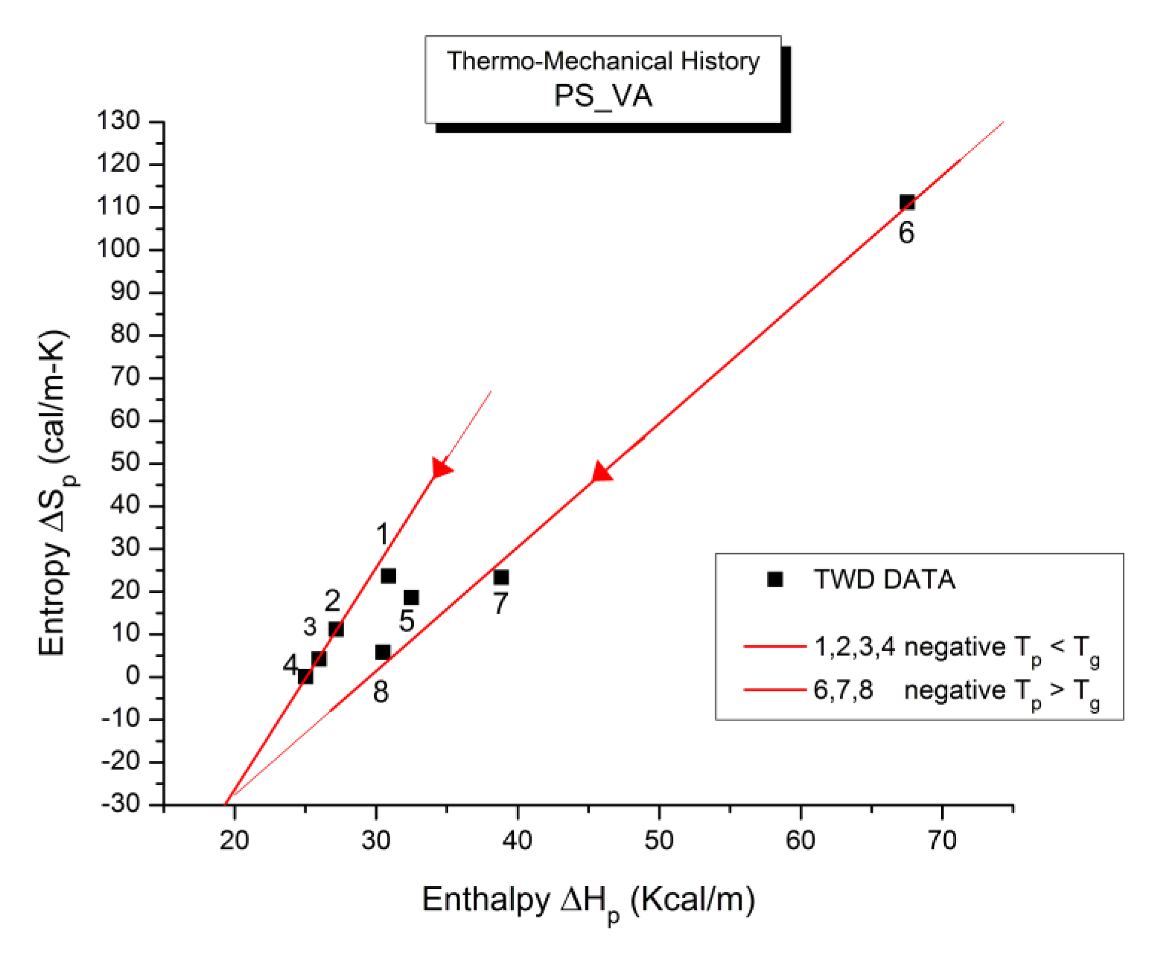
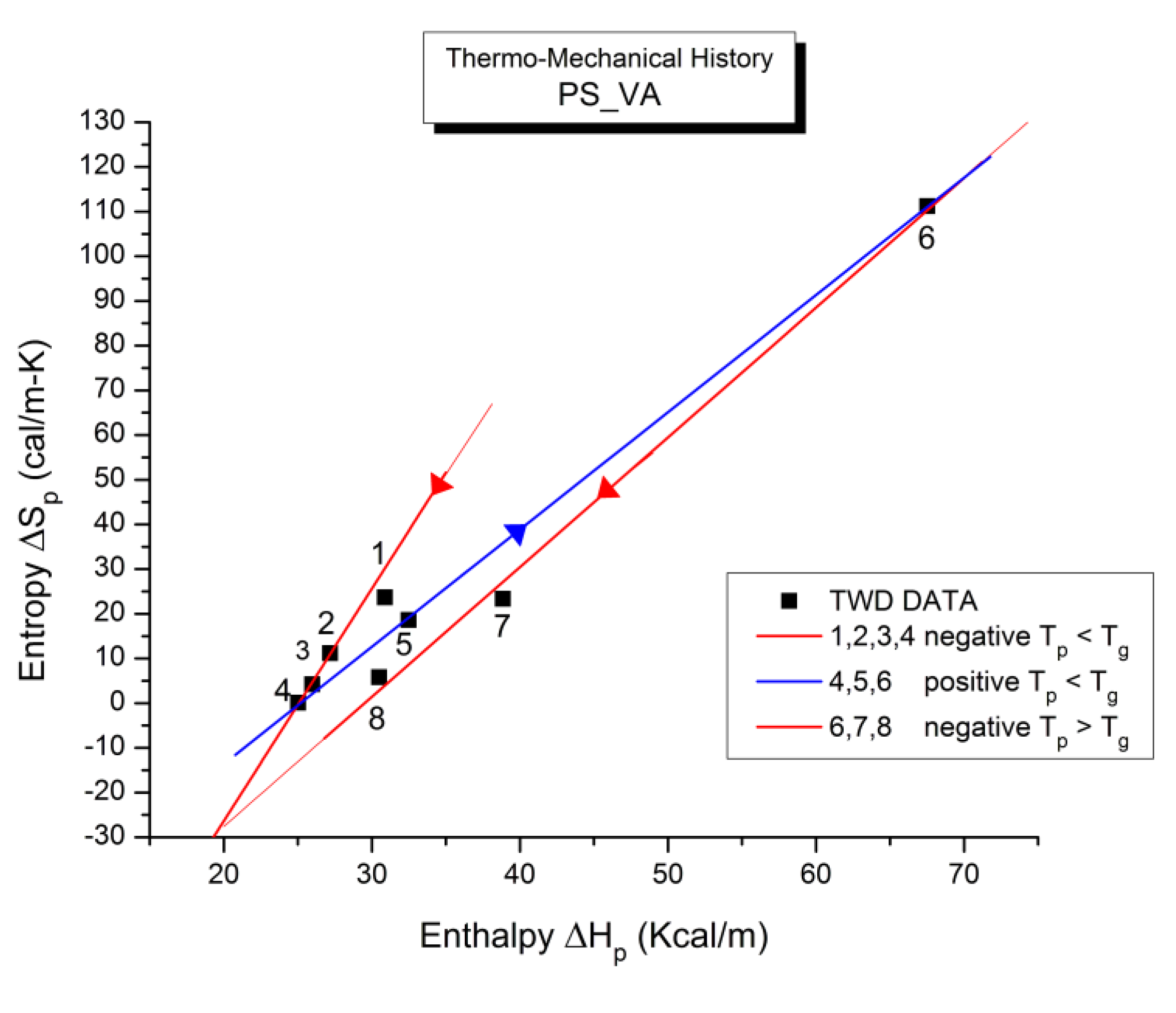
Figure 41 is the compensation search in the EE plane (Entropy vs Enthalpy). Tp is varied between 60 °C and 125 °C (the window temperature is 10 °C). The numbers near the data in
Figure 41 apply to the row numbers in
Table 1, increasing with the polarization temperature Tp. We clearly observe two
negative compensation lines in
Figure 41. The first compensation line is made up of points 1, 2, 3, and 4, all with Tp < Tg , and the 2
nd compensation line aligns points 6, 7, and 8, all with Tp > Tg ; point 5 (at Tp = 95 °C) seems to be “lost” between the two negative compensation lines. We will go back to the analysis of this PS_VA treatment in
Figure 56 and
Figure 57 and
Table 5 after the study of the relaxation maps for other thermo-mechanical histories which will have given us some insight on how to handle the analysis of these unusual and complex relaxation maps. Our first impression of the spectral lines in
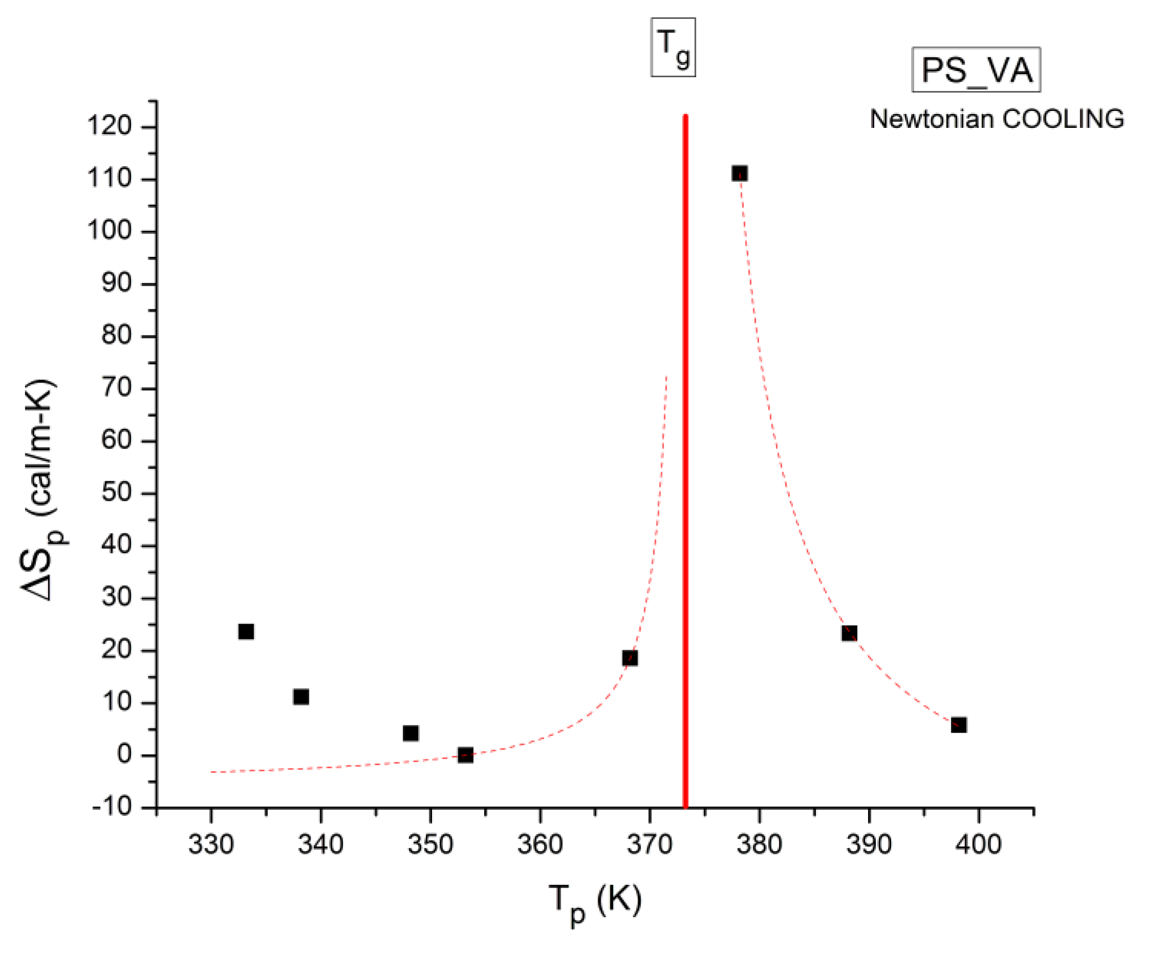
Figure 40 is that the first 5 ones, starting from the low Tp end, are more or less parallel. This is reflected in the compensation search by the closeness of their enthalpy values on the corresponding compensation line (from 31 to 25 Kcal/m). We also note that the entropy decreases from 24 cal/m-
oK to 0 (for point 4) and increases sharply to 111 for point 6.
Figure 40.
Relaxation map in the Eyring plane for a very slowly cooled compression-molded polystyrene sample with almost no pressure during cooling. The sample is called PS_VA in subsequent figures. The slope and intercept of the elementary deconvoluted relaxations provide the Enthalpy and Entropy values in
Table 1. The data are analyzed in
Figure 41,
Figure 56 and
Figure 57. .
Figure 41.
Compensation search in the EE plane for the data of
Figure 40. The numbers near the data relate to the row position in
Table 1.
Figure 41.
Compensation search in the EE plane for the data of
Figure 40. The numbers near the data relate to the row position in
Table 1.
Figure 42,
Figure 43,
Figure 44,
Figure 45,
Figure 46 and
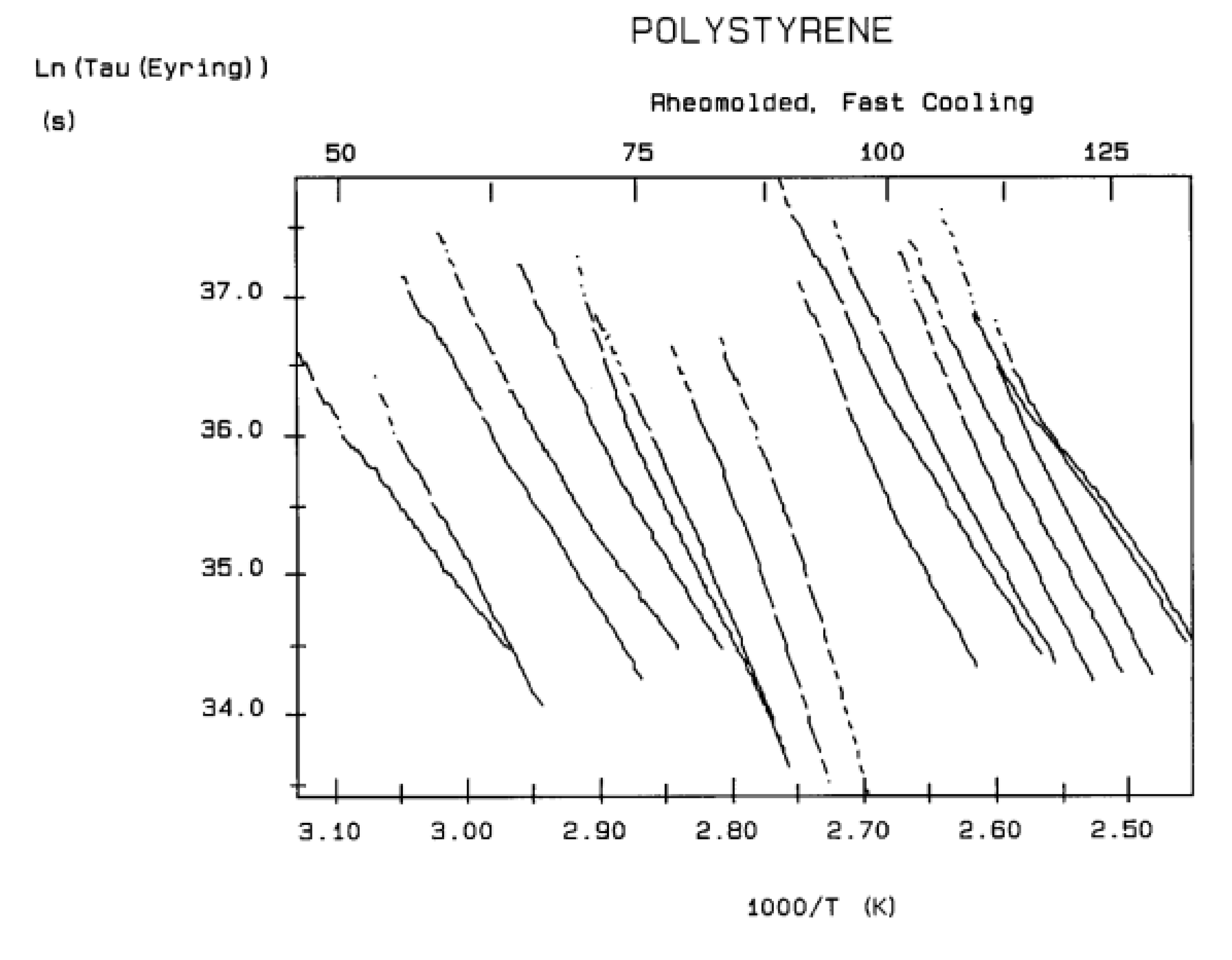
Figure 47 relate to the same polystyrene, but mechanically pressurized during a fast cooling treatment. The mechanical treatment includes the application of vibrational positive pressure to induce specific thermal history patterns, a process known as “Rheomolding” [
33]. The mold is cooled in approximately 30 seconds. The rate of cooling when the glass transition temperature is crossed is around 7 °C/sec, considerably faster than for the PS_VA treatment in
Figure 40.
Figure 42 is the relaxation map in the Eyring plane.
Figure 43 is the compensation search in the EE plane based on the Entropy and Enthalpy data of
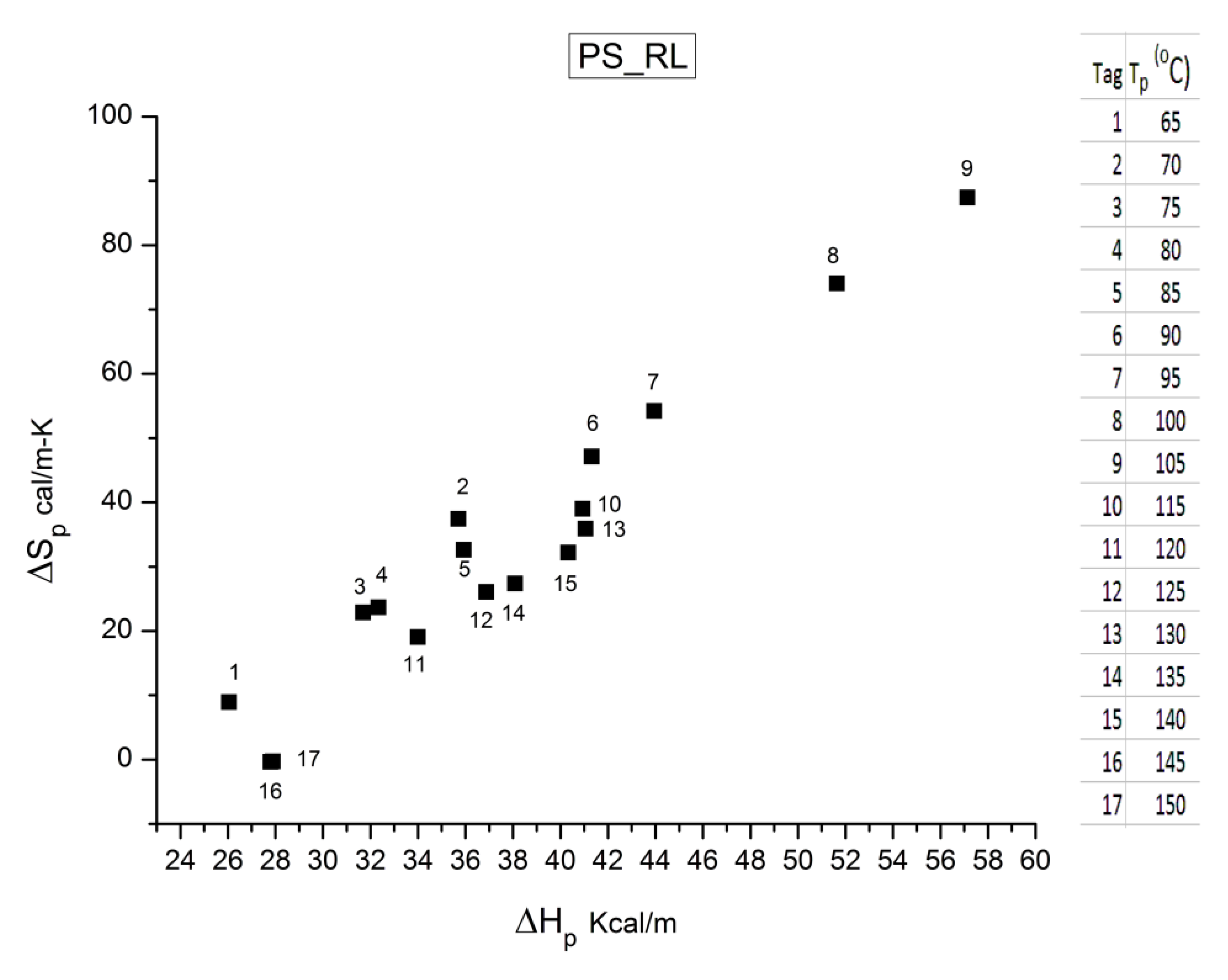
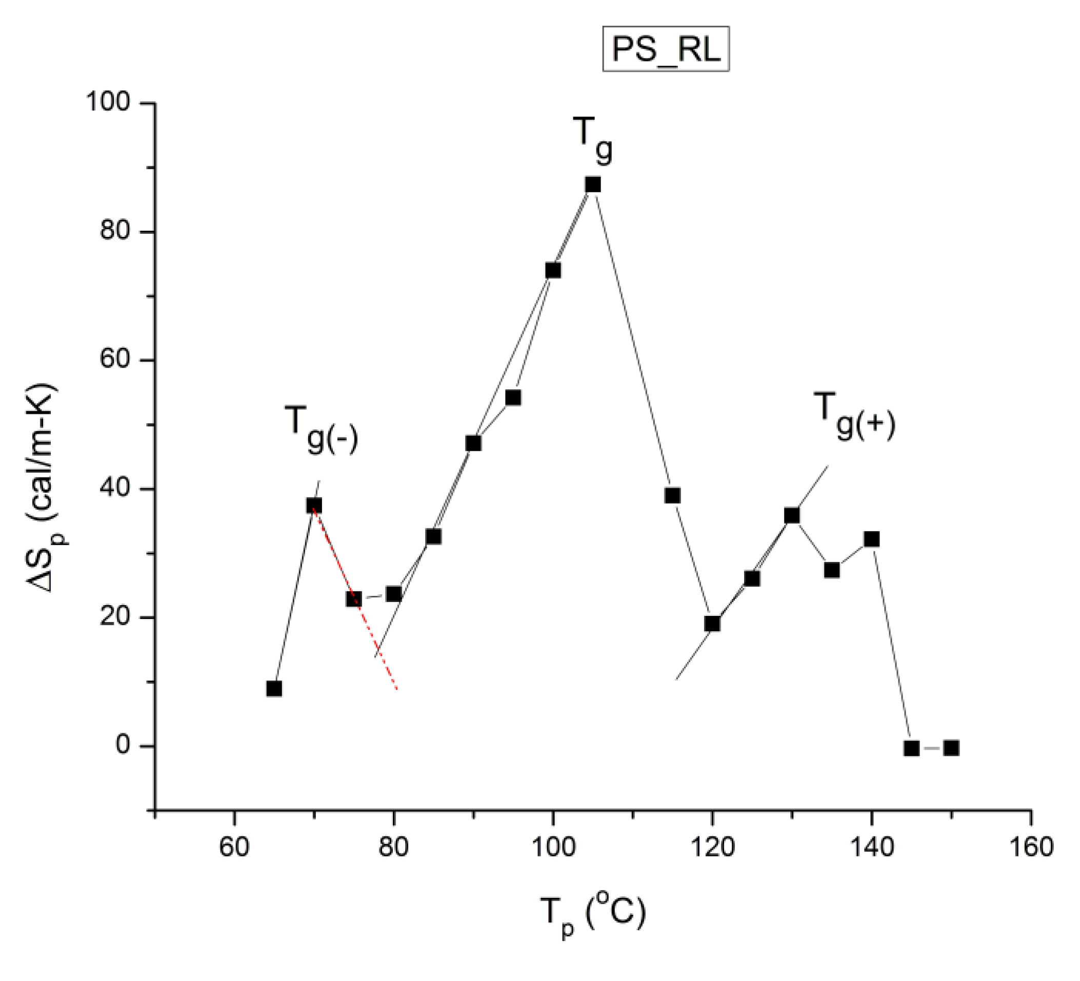
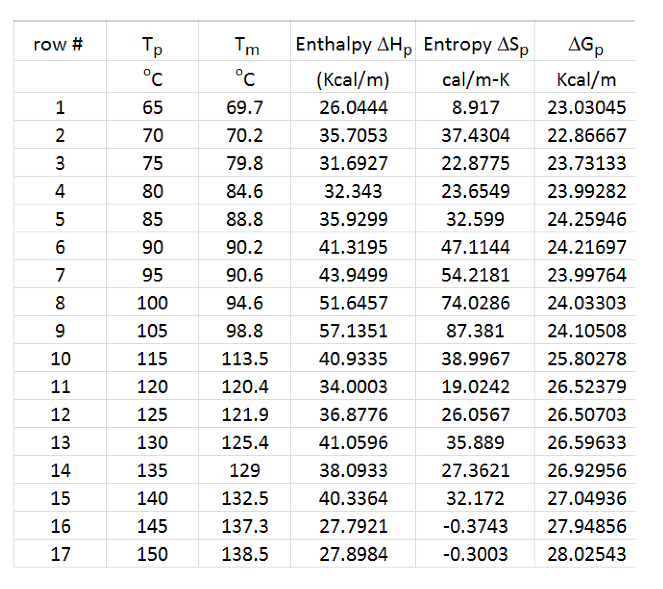
Table 2. The thermo-mechanical treatment is called “PS_RL”.
Figure 43 appears complex, unlike what is observed for stable amorphous states for which two compensation lines can be drawn passing through the data: one positive compensation line for Tp < Tg relaxations, and one negative compensation line for Tp>Tg. This cannot be the correct solution in
Figure 43 because 2 lines only would not join consecutives Tp data points, which is a sine qua non condition to define a compensation. In fact, as
Figure 44,
Figure 45,
Figure 46 and
Figure 47 will demonstrate, the situation is more complex
only apparently since we find several correlations and a network structure between the 6 compensations (3 positive and 3 negative) that are necessary to comprehend the relaxation maps in
Figure 42 and
Figure 43 Figure 44,
Figure 45,
Figure 46 and
Figure 47 illustrate our step by step method to clarify complex compensation searches, which we will only explain for PS_RL only.
Figure 42.
Relaxation map in the Eyring plane for a “Rheomolded” compression molded PS sample designated PS_RL. The sample is pressurized and vibrated during fast cooling in the mold.
Figure 42.
Relaxation map in the Eyring plane for a “Rheomolded” compression molded PS sample designated PS_RL. The sample is pressurized and vibrated during fast cooling in the mold.
In the Eyring plane the Debye relaxation times are normalized by the vibrational energy of the atoms (kT/h), where k is the Boltzman’s constant, T absolute temperature and h is the Planck’s constant. The slope and intercept of the Log τ (Eyring ) vs. 1/T provides directly the activation enthalpy, ΔHp= slope*k, and the activation entropy, ΔSp= Intercept*k ,of the elementary Debye depolarization process.
Figure 43.
Compensation search in the EE plane for the PS_RL sample of
Figure 42. The analysis appears complex. The numbers near the data(black squares) are the row numbers in
Table 2 corresponding to the Tp value (shown in the inset) during the TWD . For a simple amorphous state such a EE plot has two straight lines going through the data, a positive and a negative compensation lines intersecting at Tg, but we cannot represent such a simple solution since compensation lines should join consecutive increasing or decreasing Tp points for positive or negative compensations, respectively. The finding of the true positive and negatives compensation lines for this complex situation is shown in
Figure 45 and
Figure 46.
A compensation search looks for an affinity between successive interactive coupling relaxation modes activated at different polarization temperatures Tp. In
Figure 43, the Eyring relaxation map of
Figure 42 is converted to the EE plane variables (Entropy vs Enthalpy) , and the affinity between the relaxation modes is determined by the alignment on a straight line (the “compensation”) of the thermo-kinetic coordinates , Hp and Sp for neighboring Tp values. In
Table 2 we see that Tp was varied every 5 degrees from 65
oC to 150
oC (17 values). in
Table 2, rows 1 and 2 for Tp=65 and 70
oC, correspond to the two first relaxation lines on the left of
Figure 42. These two relaxation modes appear to cross in that figure at a Eyring relaxation time, c, and a temperature T= Tc. In the EE plane (
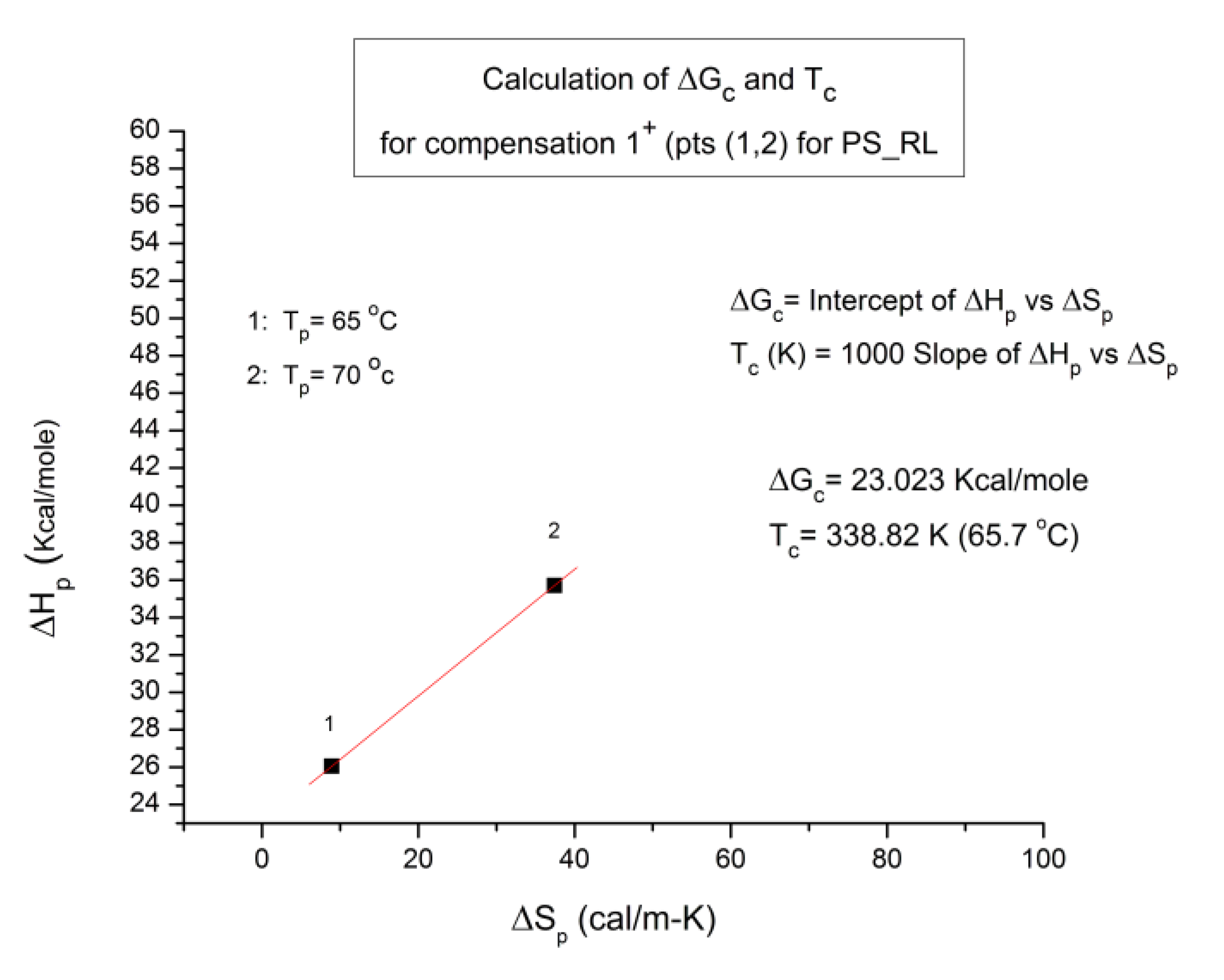
Figure 43), these two relaxation modes are points # 1 and 2. The line (1,2) is the compensation line that permits to calculate the coordinates of the compensation point of these two elementary relaxations in
Figure 42. This is done in
Figure 44, a plot of Hp vs Sp in which the x and y axes have been swapped to allow an easy determination of the compensation point in the G plane: Tc, Gc. In
Figure 44 the value of Gc is simply the intercept of line (1,2), and the Tc value (in Kelvin degrees) is equal to 1000 times the slope of line (1,2). In
Figure 43, as Tp increases beyond point # 2, one sees that #3 is not located on line (1,2) , it is below it although its Tp has increased; a clear reversal of the direction indicates the presence of a new compensation with a change of its “sign”, here between points #2 and #3. The 1
st compensation (1,2) is called “1+ ” since it is positive, while (2,3) is called “1
-“ since it is the first negative compensation (we also use the appellation C1+ and C1- to designate these compensations). As Tp continues to raise, points #3 to #9 are aligned on a single straight line forming the 2
nd positive compensation , “2+ ” (or C2+). The second negative compensation lines down points #9, #10, and #11 and is designated “2
- ” (or C2-) , and so on and so forth for the remaining points sub-grouping in compensations “3+ “ and “3
- or even in “4+ “ and “4
- in some instances. The rule followed to define the various compensation lines is that only successive points can participate in a compensation line. Sometimes we hesitate between two options because of the errors on the determination of the coordinates of the points: this happens at larger Tp values where relaxations of non-equilibrium samples occurs faster. The compensation search for the positive compensations is illustrated in
Figure 45 and for the negative compensations it is in
Figure 46.
Figure 44.
Compensation search
in the Arrhenius plane for PS_RL to find the compensation(s) in
Figure 42. Several positive and negative compensations emerge from what initially looked complex (in
Figure 43). The down arrows indicate positive compensations, the up arrows negative compensations.
Figure 44.
Compensation search
in the Arrhenius plane for PS_RL to find the compensation(s) in
Figure 42. Several positive and negative compensations emerge from what initially looked complex (in
Figure 43). The down arrows indicate positive compensations, the up arrows negative compensations.
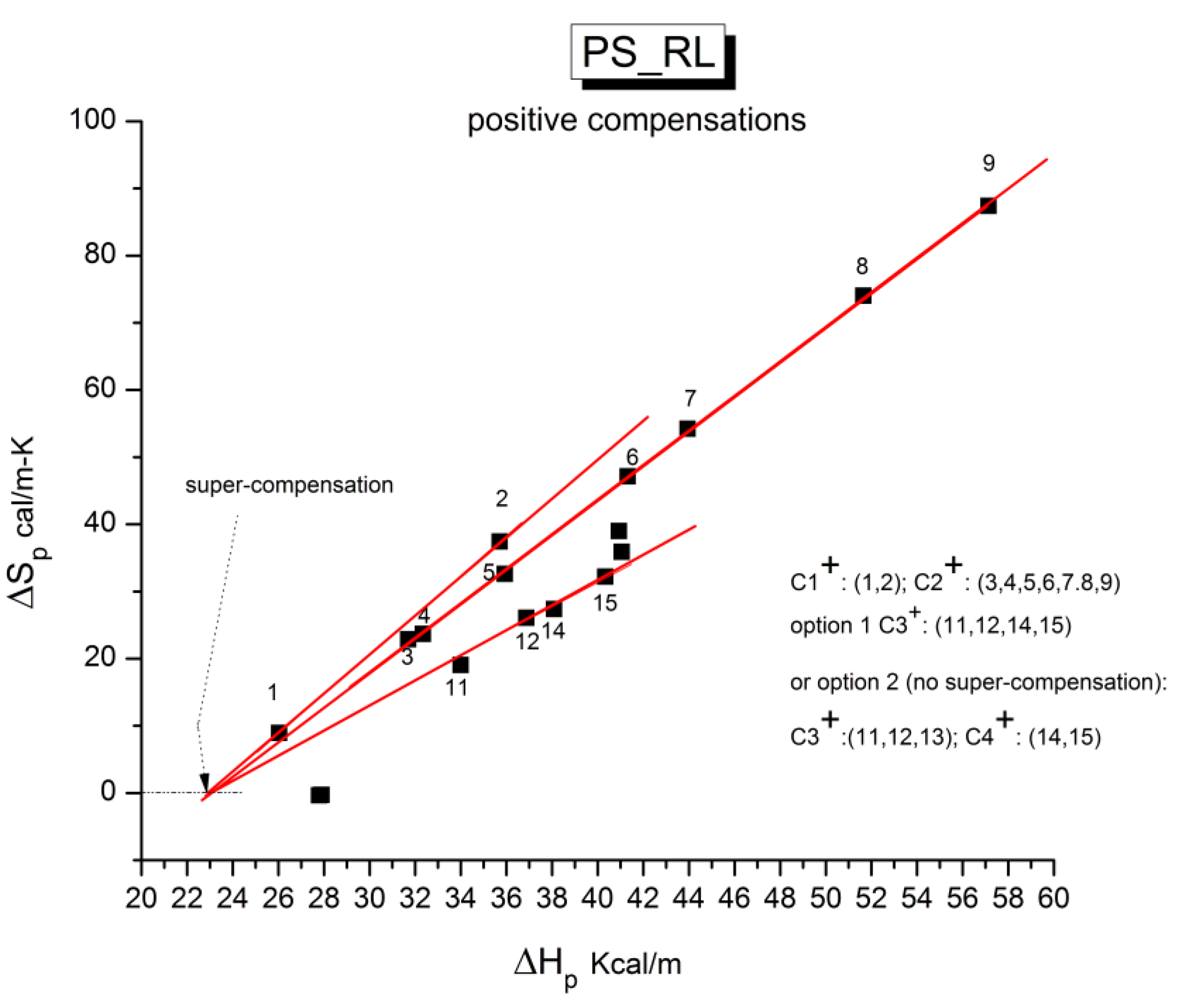
Figure 45 reveals that the
positive compensation lines (in red) appear to converge on the ΔSp = 0 axis. The corresponding value of ΔHp at the intercept point is 23 kcal/mole. This point is fully independent of the value of Tp : it is a
super-compension, the compensation of all the positive compensation lines for sample PS_RL. When we say for “all” the positive compensations, we should add that this is 100% sure for compensations C1+ and C2+, but that a different split of the points is possible for C3+ as shown in the inset of Fig.45: either C3+ = (11,12,14,15) or C3+ = (11,12,13) and C4+ = (14,15).
Figure 45 shows the 1
st choice that has only 3 compensation lines.
Figure 45.
Compensation search in the EE plane for PS_RL showing the
positive compensation results only (lines joining successive T
p points with increasing values of ΔS
p and ΔH
p). The 3 positive compensation lines converge to a “super-compensation” point (whose y-coordinate is ΔS
sc(+) = 0) for option 1. For option 2, with 4 compensations, only 3 of them super-compensate. The analysis for the negative compensations is in
Figure 46.
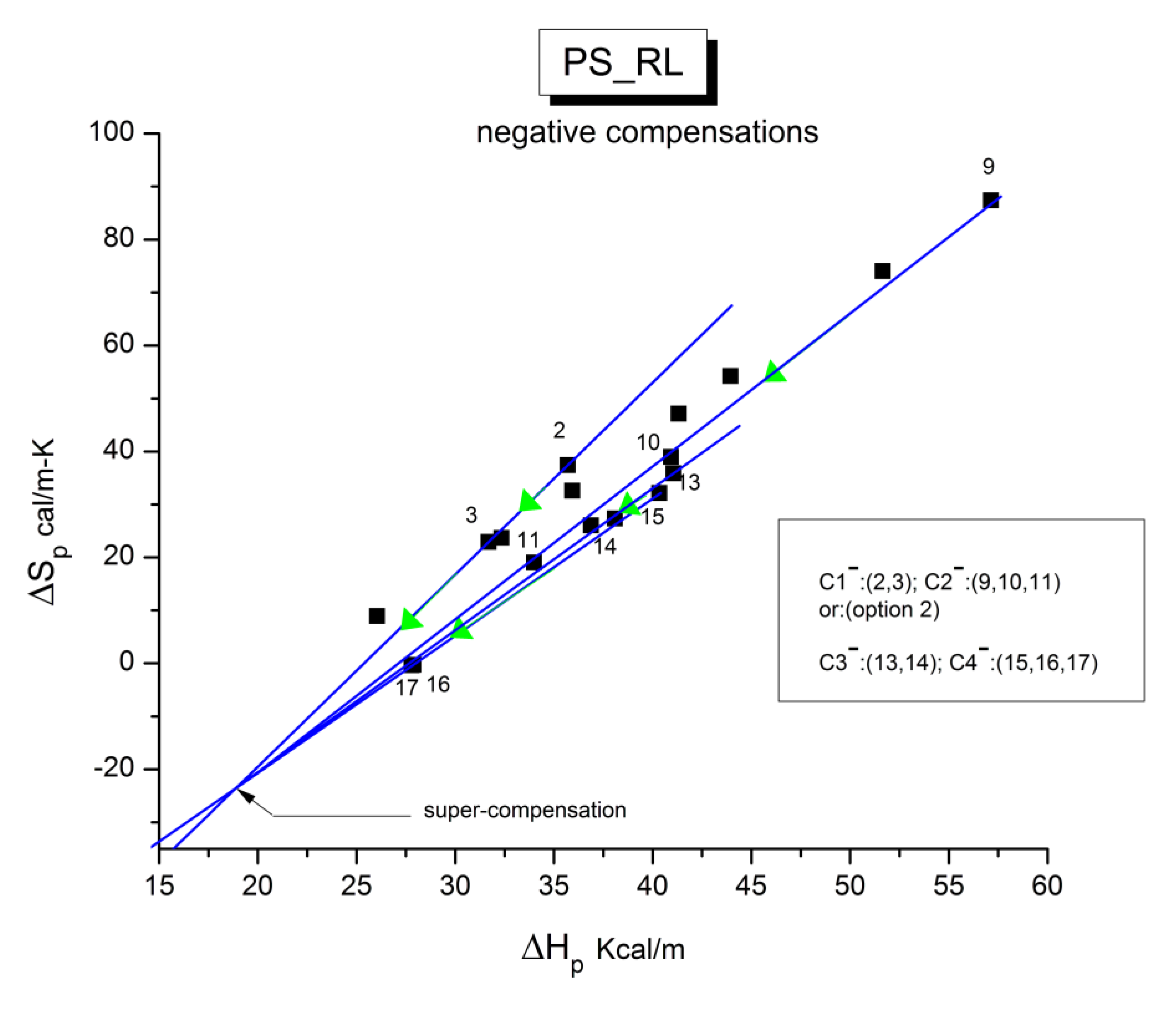
Figure 46 concentrates on the points interacting to generate negative compensation lines. This analysis is a little bit more difficult because there are fewer points to define the lines accurately. Nevertheless, it is possible to draw with confidence three negative compensation lines (option 1) or 4 compensation lines (option 2) and in the later case they themselves converge with confidence to a super-compensation (ΔHc=18,8 Kcal/n, ΔSc=-23 cal/m-K).
Figure 46.
Compensation search in the EE plane for PS_RL showing only the
negative compensation results of the analysis conducted in
Figure 43. In option 2, the 4 negative compensation lines converge to a single point, a super-compensation point whose ΔHpc(-) =18.8 Kcal/m and ΔS
pc(-) = -23 cal/m-K. For option 1, with C3- = (14,15,16,17)), there are only 3 negative compensations and the super-compensation is defined with less confidence (r
2=0.988). For option 2, with C3- and C4- defined in the inset, the convergence to a super-compensation is established with confidence (r
2=0.9987). .
We summarize in
Table 3 the results of the regressions of the compensation lines (ΔSp vs ΔHp) shown in
Figure 45 and
Figure 46 with ΔSp in cal/m-K- and ΔHp in kcal/m.
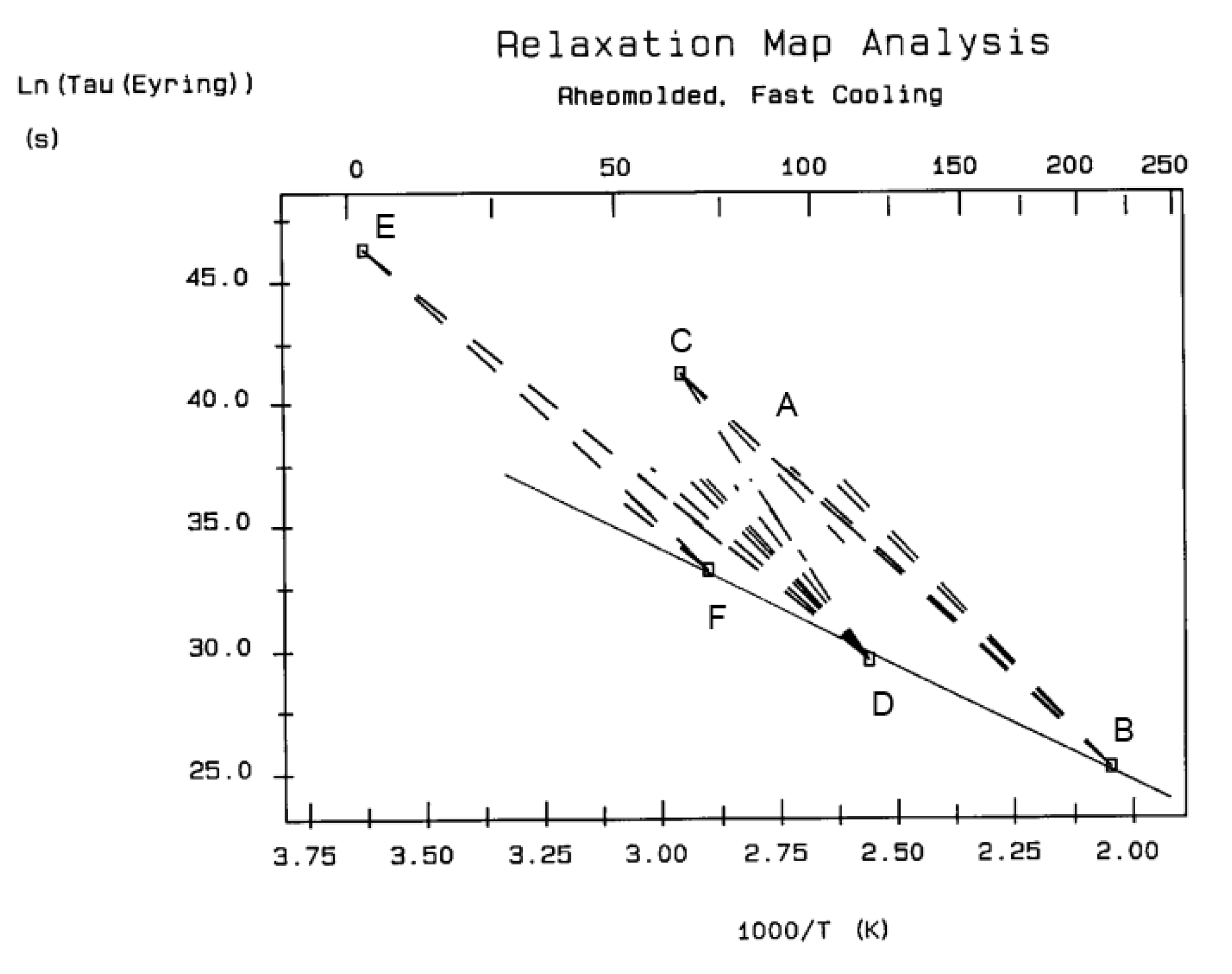
Figure 47.
Schematic reconstruction for PS_RL of the compensations of the spectral lines in
Figure 42 following the compensation search results of
Figure 45 and
Figure 46. This graph shows the full Debye spectral lines for the 3 positive compensations (with F,D,B the aligned compensation points); the spectral lines for the negative compensations are only visible for the lower Tp compensation points (E,C) and not for compensation point A.
Figure 47 represents a summary of our complex compensation search, displaying the interactive coupling map of the relaxations revealed at different Tps. The positive compensation points are shown at F,D and B in order of increasing Tp. The line passing through F,D and B is the super-compensation line whose intercept and slope provide the coordinates of the super-compensation point of the positive compensations. Note that we have drawn no line through the negative E, C and A compensation points because the spectral lines for A have not been drawn up. Yet, this negative super-compensation line can be imagined passing through E and C and would appear to be parallel to the positive super-compensation line FDB. In other words, all the compensation points and the super-compensation lines appear to create a macro network where the local spectral lines collectively belong, showing their collective dependence. We will explain this concept in the next figures below (
Figure 48,
Figure 49,
Figure 50,
Figure 51,
Figure 52,
Figure 53,
Figure 54 and
Figure 55). For this we will work in the ΔGp(T) plane representation of the TWD relaxation map( [
16], p. 79 of [
5]), where ΔGp(T) is the Free Energy of depolarization at T of the elementary Debye relaxation after polarization at Tp according to the TWD protocol: ΔGp(T)= ΔHp - T ΔSp in the ΔG plane.
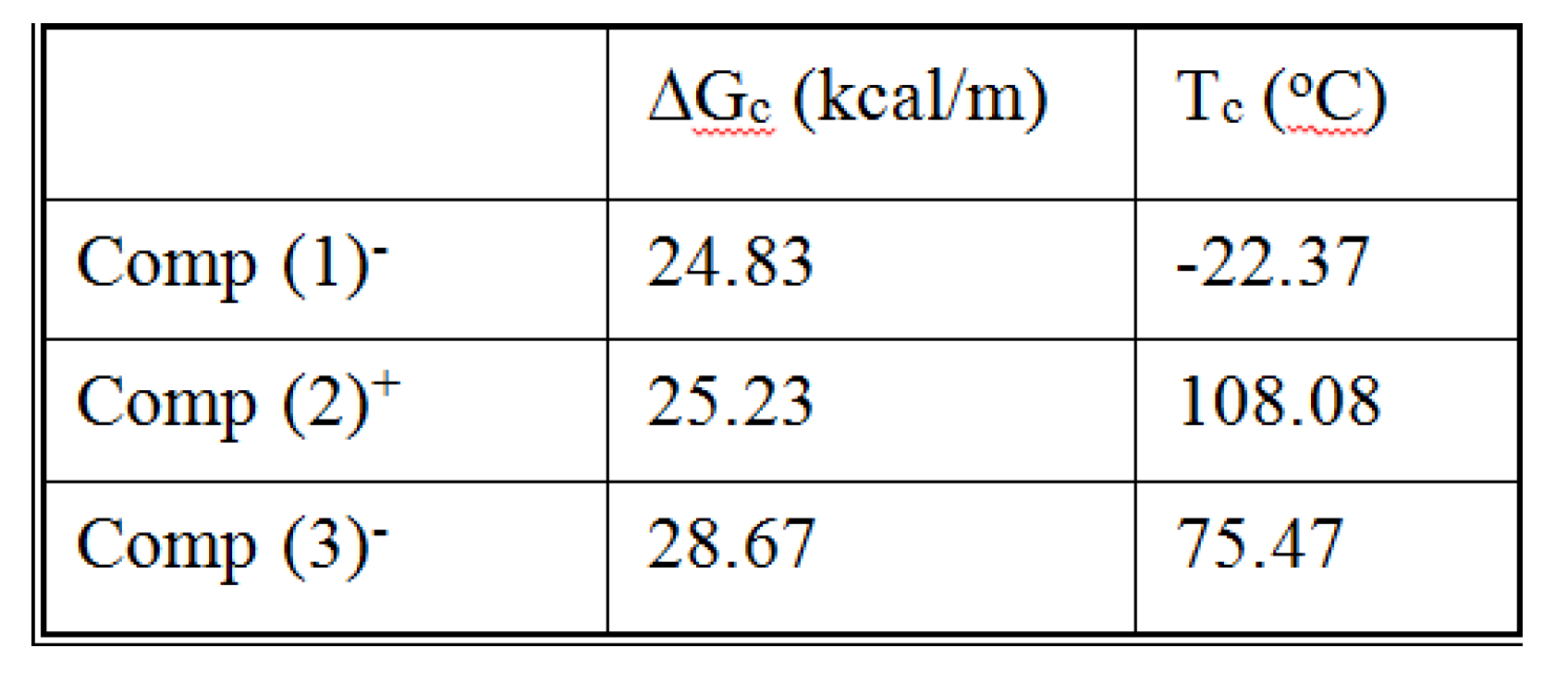
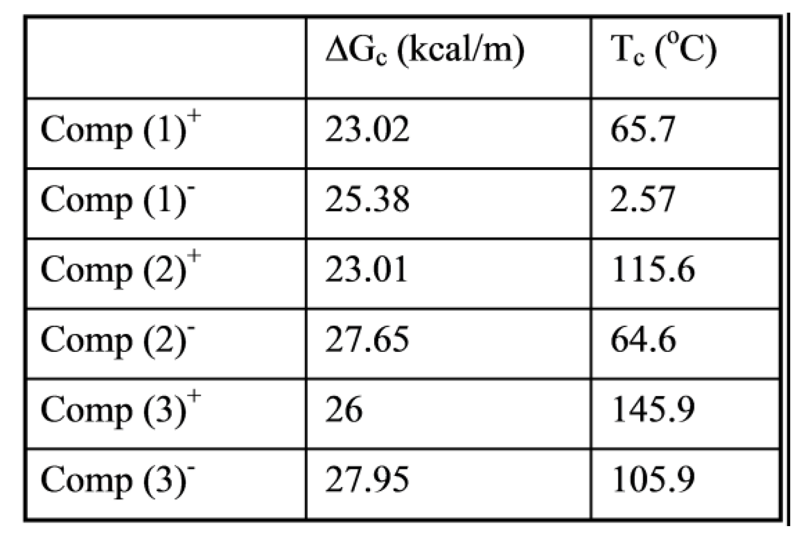
Table 3 provides the intercept and slope of the linear relationship between ΔSp and ΔHp for the compensation lines . The Free Energy at each of the compensation points, ΔGc, and the temperature of compensation, Tc, can be calculated from the value of the slope, Sp, and the intercept, Ip, of the compensation lines when they are rewritten as ΔHp = Ip+Sp ΔSp and with the conversion of the energy units for enthalpy and entropy to be the same, we obtain: ΔGc = Ip and Tc(K)= 1000 Sp. Their values are tabulated in
Table 4 for each of the positive and negative compensations.
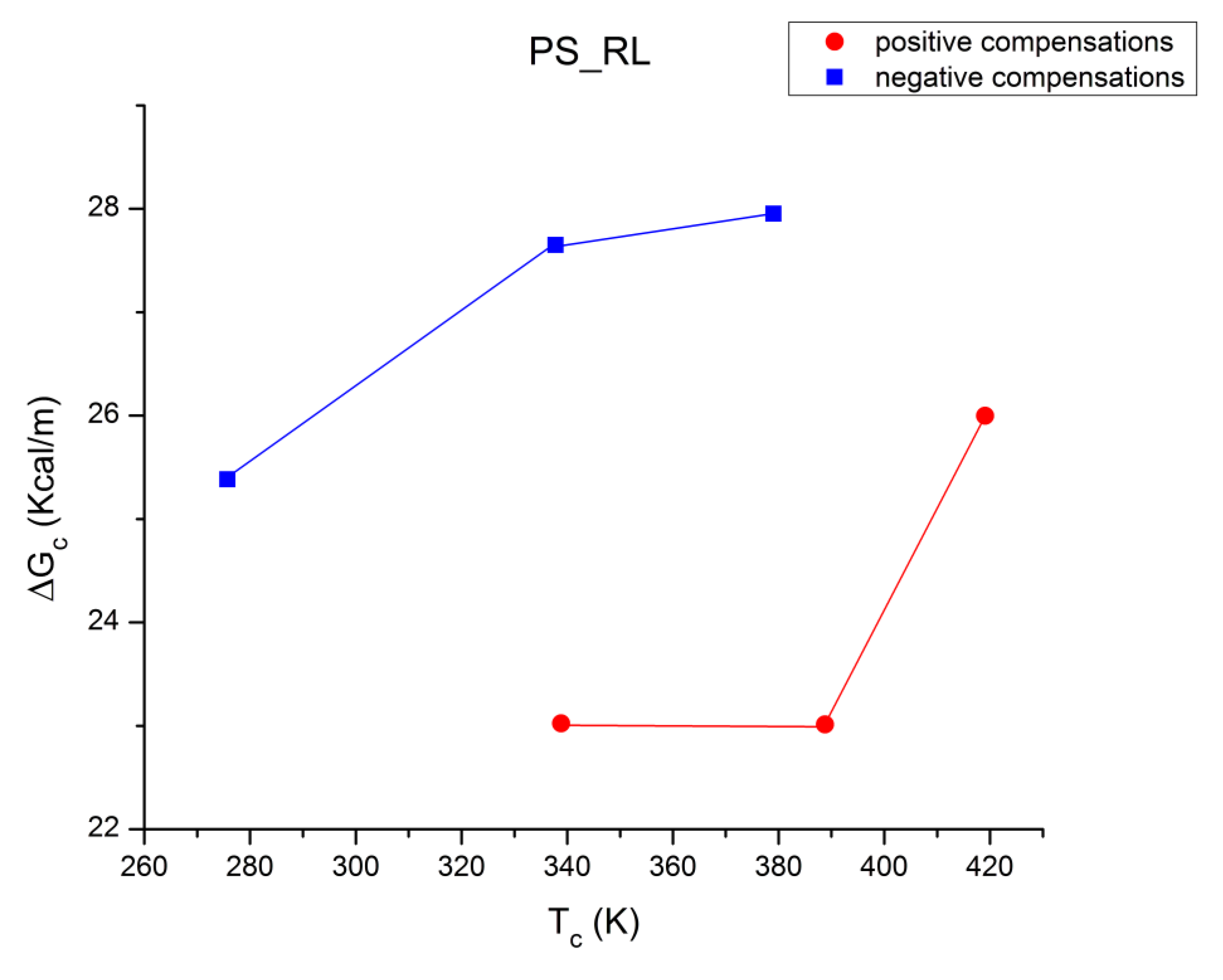
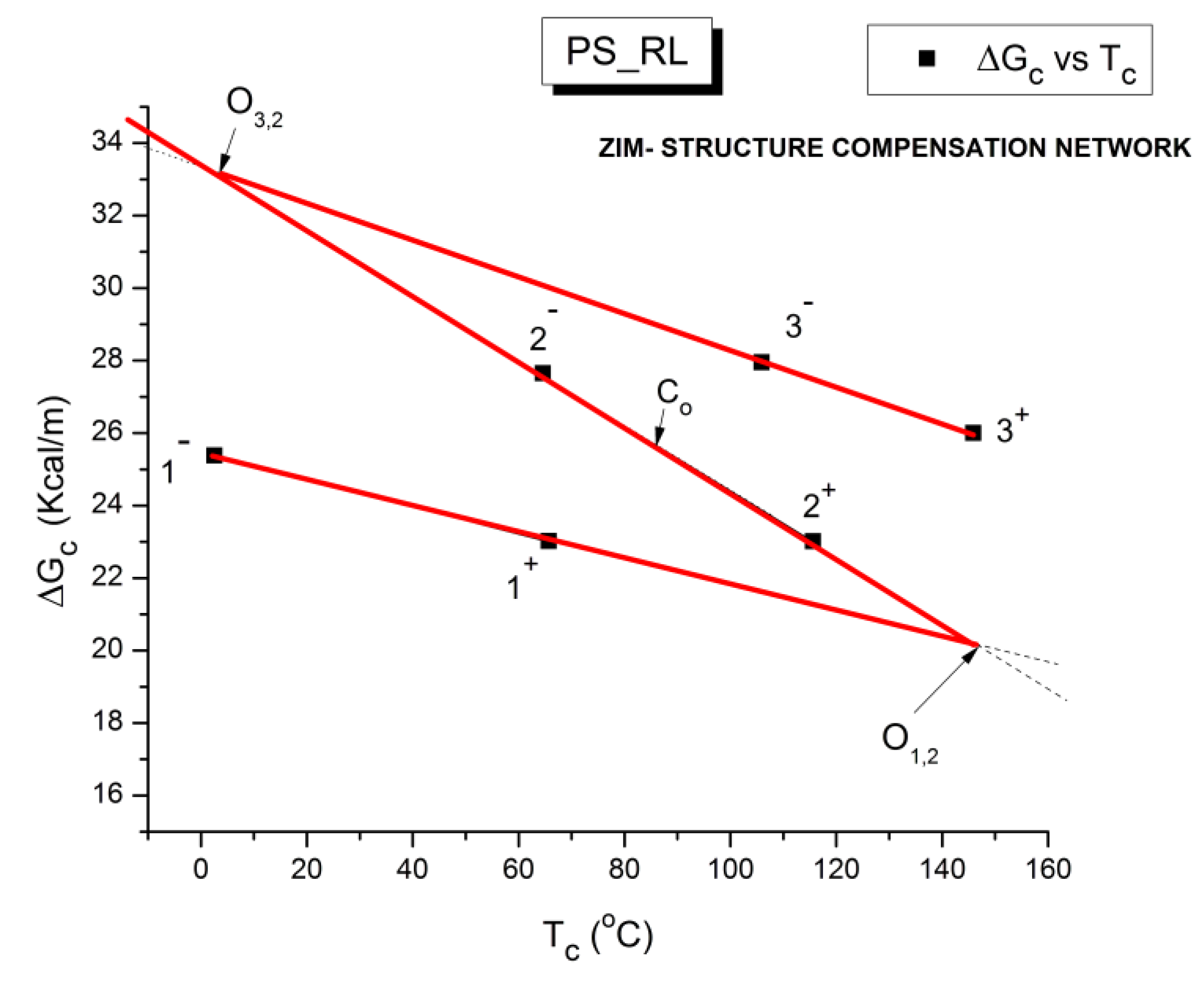
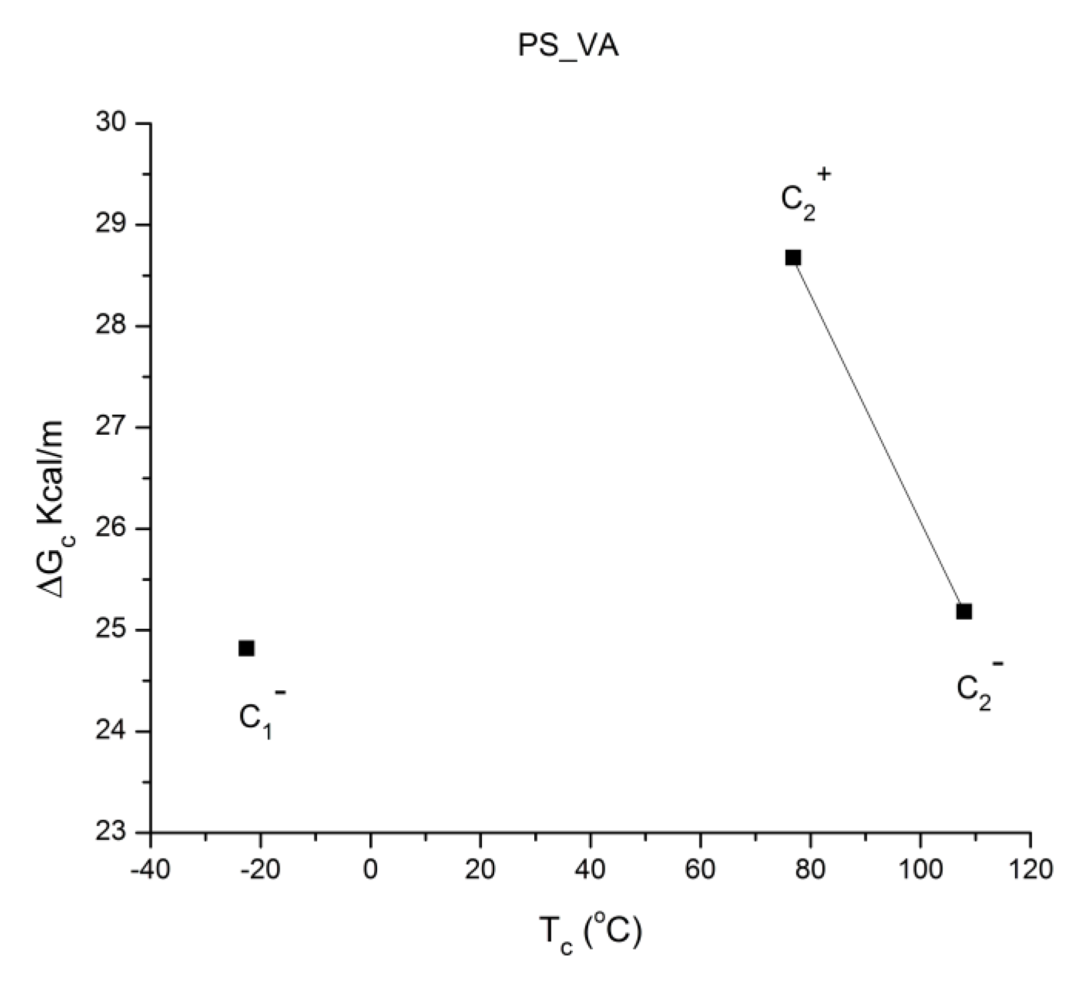
Figure 48 is a plot of Gc vs. Tc for the 6 compensations in
Table 4, using a change of color to differentiate the positive (red, bottom) from the negative (blue, top) compensation concave curves. One sees that Tc increases as the Tp range of the points belonging to the sub-group increases. The trace going through the points is monotonous for both “polarities”, but their curvature is the opposite, concave downwards for the top curve, concave upwards for the bottom one. The 2 traces of
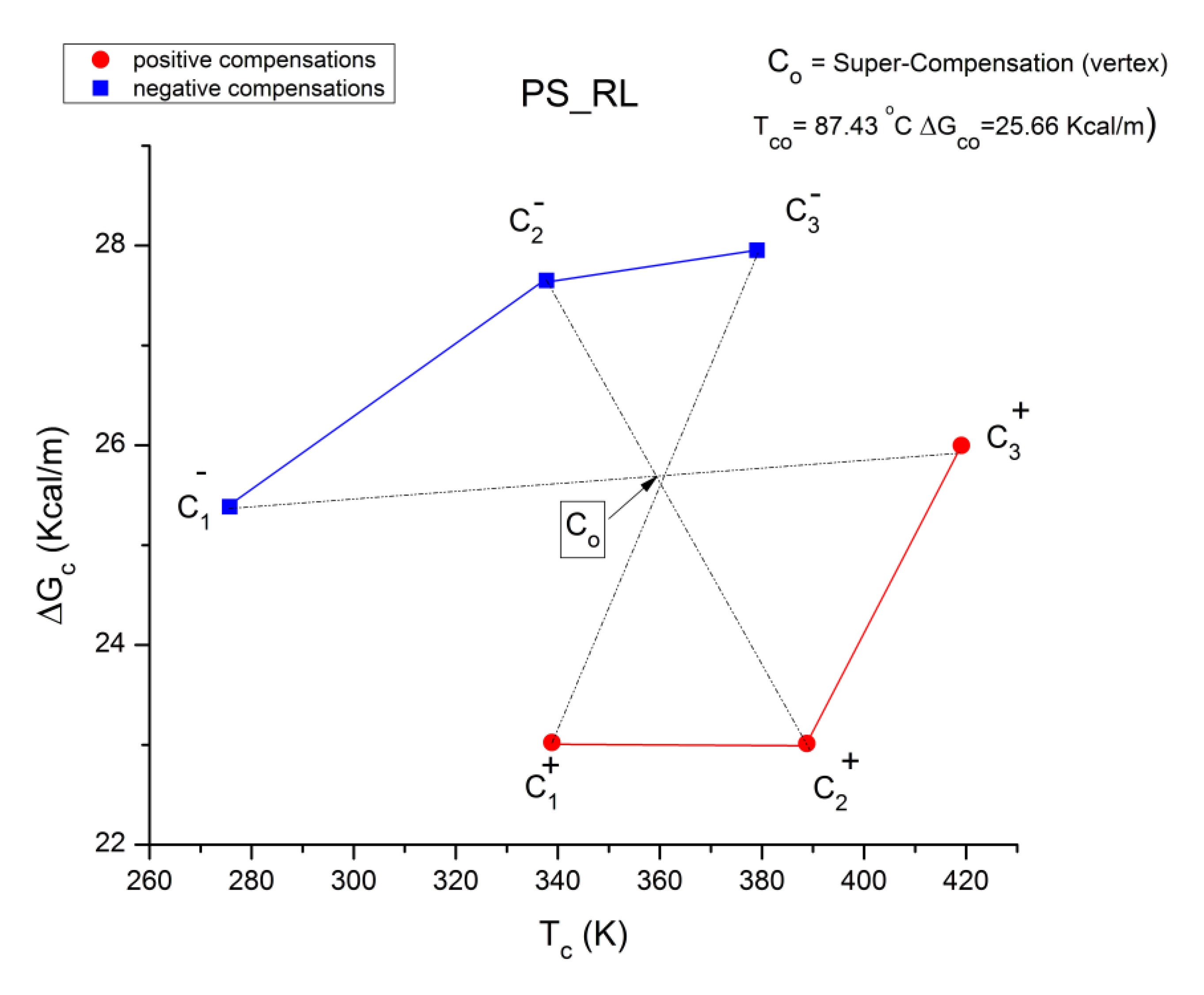
Figure 49 link points with the same polarity, positive or negative, just like
Figure 45 and
Figure 47 separated the polarities, trying to determine correlations within a given polarity: we did find the super-compensation character of the compensation lines within each polar group. In the following figures,
Figure 49,
Figure 50,
Figure 51,
Figure 52 and
Figure 53, we investigate possible correlations between the compensation points across polarities. For instance, in
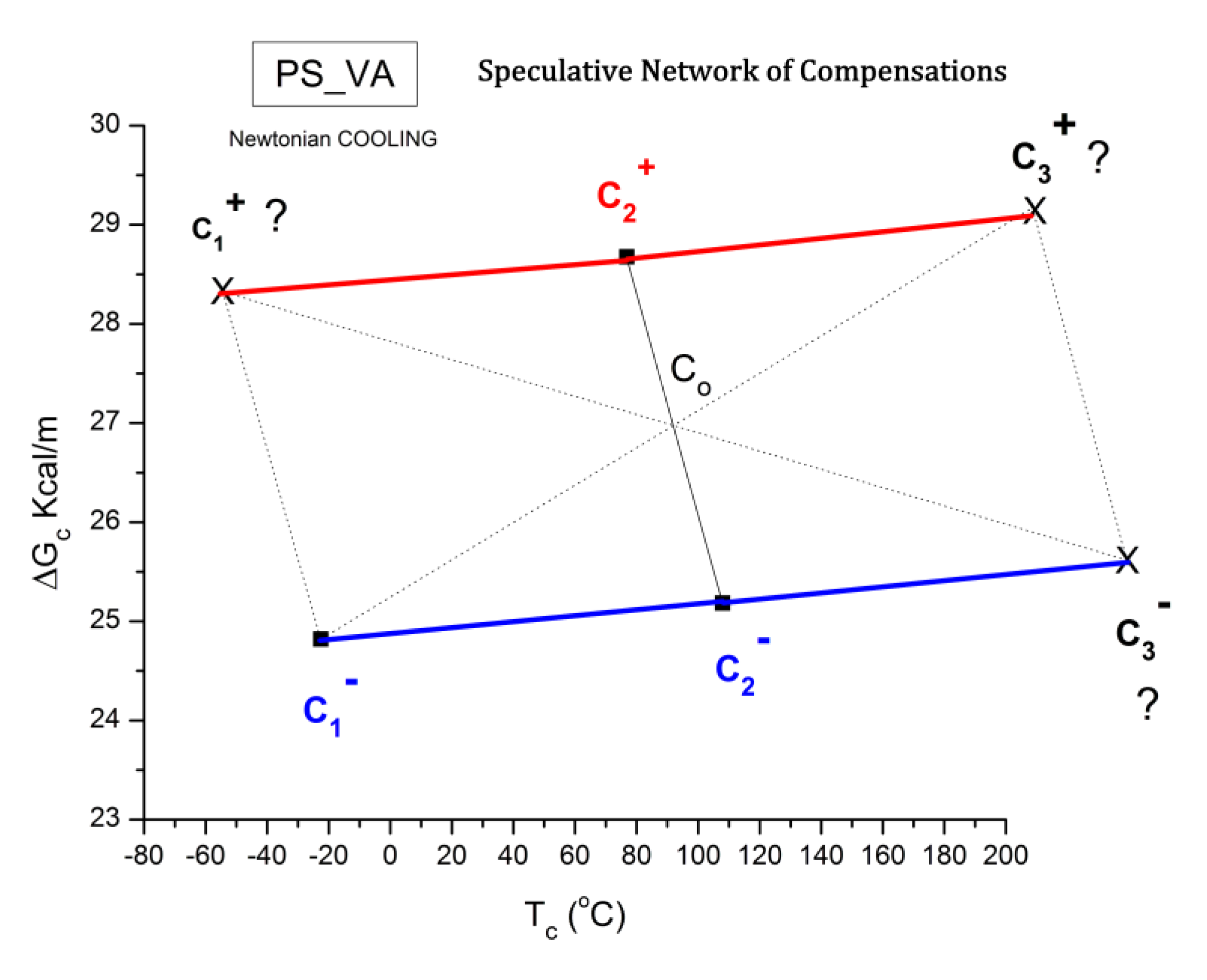
Figure 49 we show that the lines joining the “cross-compensation” points, such as C1+ and C3- or C3+ and C1- cut each other at a point that belong to the line joining C2+ and C2-. In other words, the point designated Co in
Figure 49 is a super-compensation point for the cross-polarity network of compensation points, i.e. the vertex of a pencil of lines formed by the 3 cross-polarities lines C1+C3-, C2+C2- and C1-C3+.This appears quite a remarkable property of the depolarization process of a Rheomolded sample occurring over time as temperature follows the TWD sophisticated protocol (
Figure 3) and at the same time releases the internal stress induced by the thermal-mechanical treatment. The coordinates of Co, the super-compensation point Is Gco = 25.66 Kcal/m , Tco = 87.43
oC, which is 12.57
oC below the Tg of PS.
Figure 48.
Plot of ΔGc vs. Tc for the 6 compensations in
Table 4. Red, bottom)curve: positive compensation points. Blue, top curve: negative compensation points.
Figure 48.
Plot of ΔGc vs. Tc for the 6 compensations in
Table 4. Red, bottom)curve: positive compensation points. Blue, top curve: negative compensation points.
Figure 49.
Possible correlations between the compensation points across polarities.
Figure 49.
Possible correlations between the compensation points across polarities.
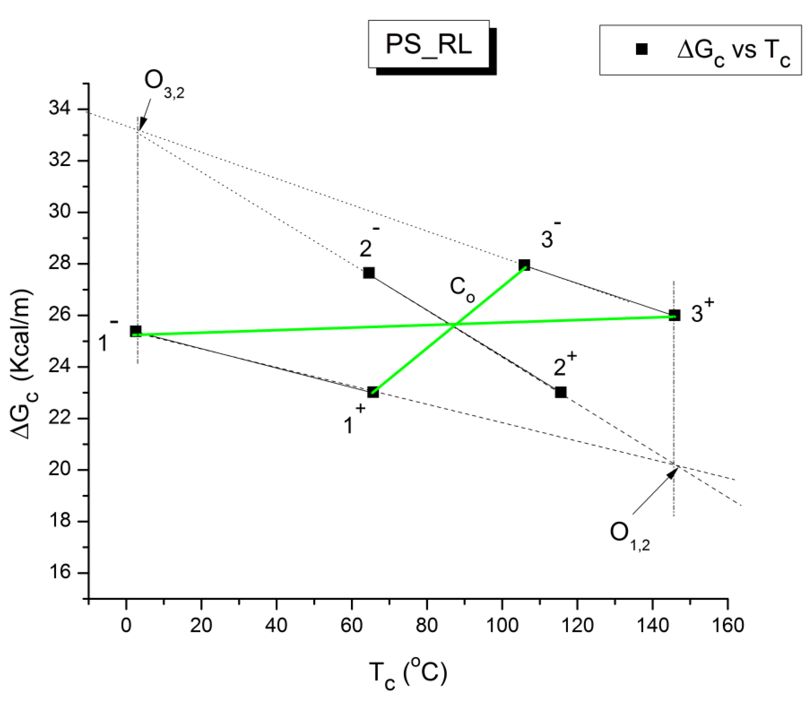
Figure 50 is an extension of our exploration in
Figure 49 of the geometrical features characterizing the network of the compensation points. We have expanded the number of links to include C3+ C3- and C1+C1- , C2-C2+ being already included from the previous figure. We also extended these 3 links so that they could cut each other. C1-C1+ cuts C2+C2- at point O12 and C3-C3+ cuts C2+C2- at point O32. The new remarkable feature is that O12 and O32 are found vertically below and above C3+ and C1-, respectively. This may indicate that the position of the points in the geometrical network respond to symmetrical rules of dependence. We are aware of the possible errors in the determination of the coordinates of the compensation points, which is done at the beginning by regressions of the Debye elementary relaxation lines in the Eyring plane (
Figure 42), far from being perfect straight lines even visually, followed by new regressions in the EE planes after the selection of the compensation sub-groups (
Figure 45 and
Figure 46). This makes the quasi-perfectness standing of the geometrical features in
Figure 50 almost impossible to accept. At least some imperfectness should exist. This imperfectness may be actually present and could have resulted, in fact, in distorting slightly the network symmetry so that C1+ should align horizontally with C2+, C2- should also align horizontally with C3- and C3- should align vertically with C2+. in
Figure 50, these alignments are almost there, like C2- already aligns vertically with C1-, as well as O32 with C1- and O12 with C3+ as already mentioned above. This is as if we had discovered a crystal-like perfection of the alignment of the compensation points in the network of compensations. This finding is new and was not presented in the book[
5], although the experimental evidence was already included(II.4.2 of [
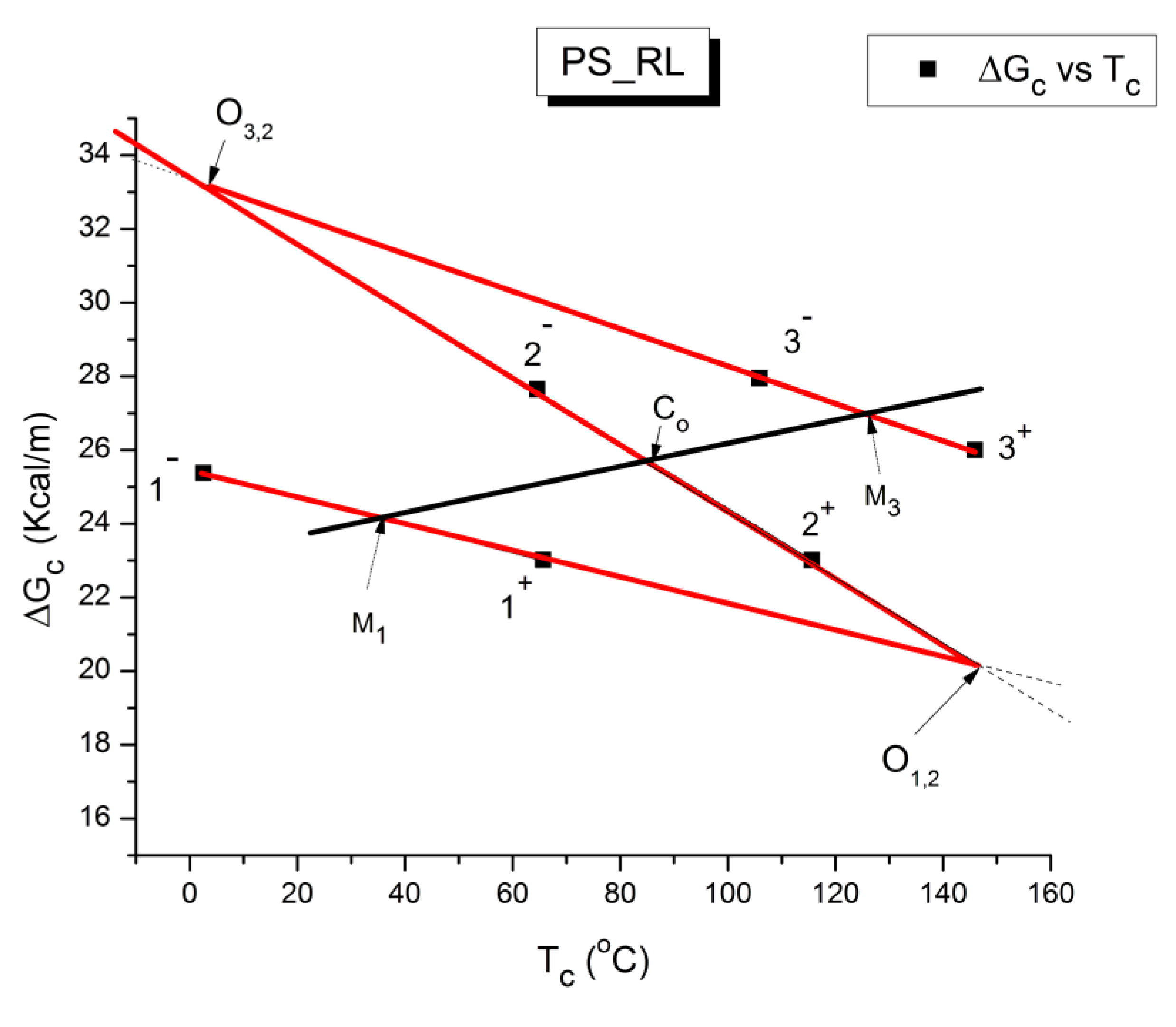
5]). Obviously, these new findings remain at the stage of speculations and the standard scientific procedure should be applied to affirm or disapprove such new discoveries. Other geometrical particularities of the “structure of the compensation network” are noticeable in
Figure 51:
- -
the line (black) joining the middle of the segment C1-C1+, M1, to the middle of C3-C3+, M3, passes through Co, the vertex of the pencil of lines C1+C3-, C1-C3+,C2+C2-.
- -
line C1-C2- is parallel to line C1+C3+ and M1CoM3
- -
distance O32C2- = distance CoO12
Figure 50.
Other possible correlations between the compensation points across polarities. See text.
Figure 50.
Other possible correlations between the compensation points across polarities. See text.
Figure 51.
Z-structure type correlations between the compensation points across polarities.
Figure 51.
Z-structure type correlations between the compensation points across polarities.
Figure 52.
The Z-structure (or ZIM) of the compensation points of a sample brought out of equilibrium by a thermal treatment has geometrical features characteristic of the thermal treatment variables (pressure, vibration frequency and amplitude, cooling rate [
8,
34]). The Z network has a center Co and its asymmetry can be described by the difference between the vertical distances O32C1- and C3+O12. .
Figure 53.
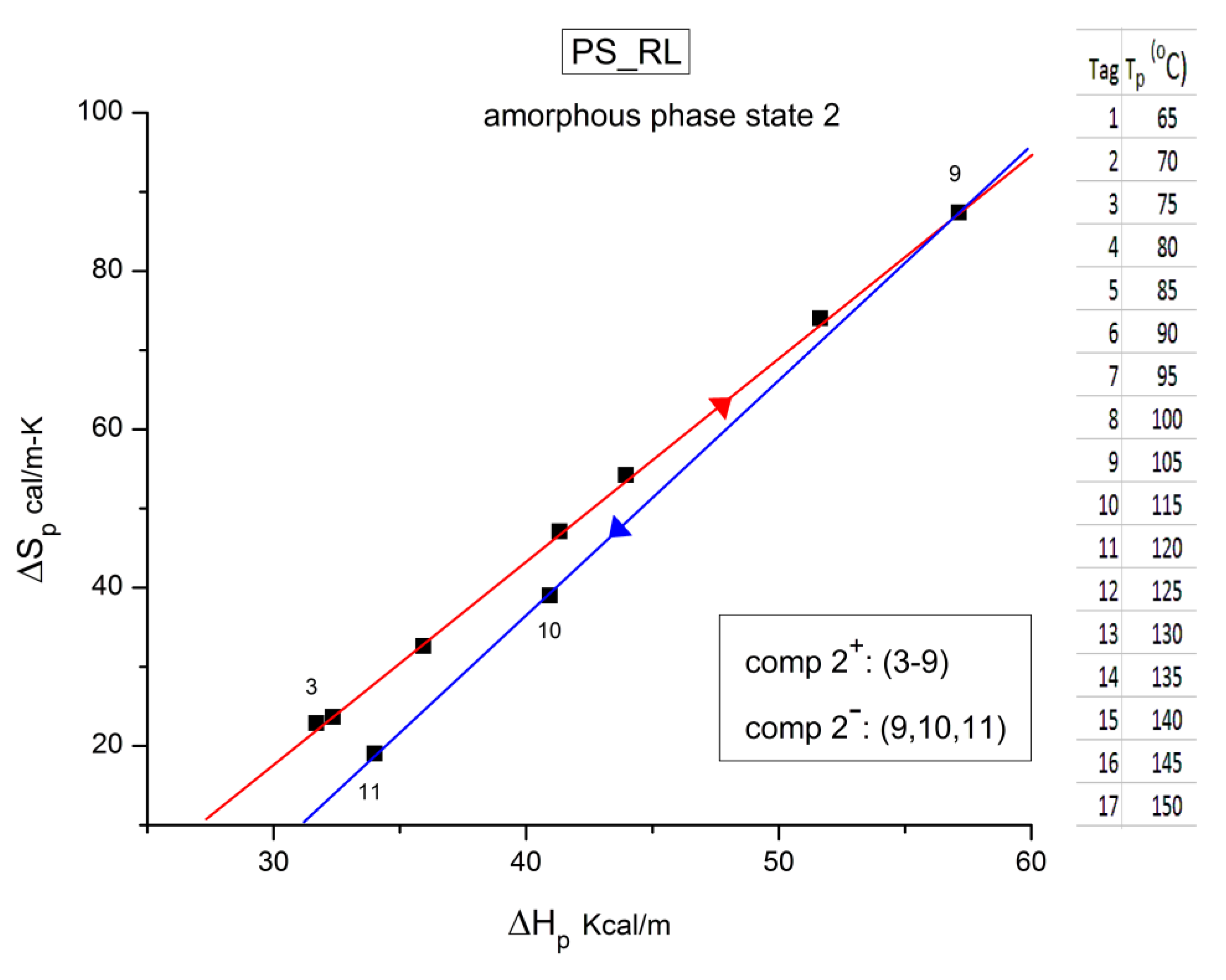
The two compensation lines, “positive” (points 3 to 9 at the top) and “negative” ( 9,10,11) at the bottom) define the behavior of amorphous phase “2”. Their intersection occurs at Tg providing ΔHg and ΔSg.
Figure 53.
The two compensation lines, “positive” (points 3 to 9 at the top) and “negative” ( 9,10,11) at the bottom) define the behavior of amorphous phase “2”. Their intersection occurs at Tg providing ΔHg and ΔSg.
Another important particularity of the network of compensation points, of great significance for the properties of the amorphous state of polymers, is its ability to determine the Tg of the amorphous phases in polymers. We will refer to both
Figure 52 and
Figure 53 to explain this important finding. In
Figure 52 we have redrawn the same graph that was used in a couple of previous figures but have removed all un-necessary details in the previous graph to let reveal the presence of the so-called “Z-structure” of the network of compensation points. The graph shown is actually a Z looked at in a mirror, which is the reason we called it the ZIM structure. A similar Z - structure is already observed at the scale of the elementary Debye relaxations to characterize a Tg transition (
Figure 11), but in
Figure 52 we are working at a different scale, the scale of the compensation lines, not the elementary relaxations, and yet, we observe a Z- structure associated with the 3 transitions characterizing phase 1, phase 2 and stay 3; in a way,
Figure 52 is the higher stage of a Russian doll assembly that repeats itself at different scales.
Figure 53 is a plot of ΔSp vs. ΔHp limited to the positive and negative compensations C2+ and C2-, with a red and a blue line passing through the positive or negative data points, respectively. It can be shown [
16] that the intersection of these compensations corresponds to the Tg state of the amorphous state relaxing via the process of TWD. We visually see that the intersection is approximately for ΔHp= 60 Kcal/m and ΔSp= 90 cal/m-K. These values are the enthalpy and entropy of activation of the mode of relaxation triggered by the polarization at Tp=Tg: we designate them ΔHg and ΔSg. We also explain in previous communications (p. 73 of Ref. [
5] and [
16]) how to find the value of Tg from the thermos-kinetics values of the amorphous phases of the positive and negative compensations. The 1
st method is based on the assumption that at Tg: ΔGg= (ΔGc+ + ΔGc-)/2 and since for all Tp : ΔG = ΔHp-T ΔSp, then for Tp = Tg we have ΔGg = ΔHg – Tg ΔSg In other words:
Equation (13) summarizes the first method to find the value of Tg from TWD to characterize an amorphous phase. It can be used in conjunction with the values of ΔGc+ and ΔGc- from
Figure 52 applied to compensations 1, 2 and 3 and the values of ΔHg and ΔSg calculated similarly to the way explained for phase 2 in
Figure 53 to find the Tg for phases 1 and 3 besides phase 2.
The second method to determine Tg from the results in a relaxation map is explained with regard to
Figure 54 and
Figure 55.
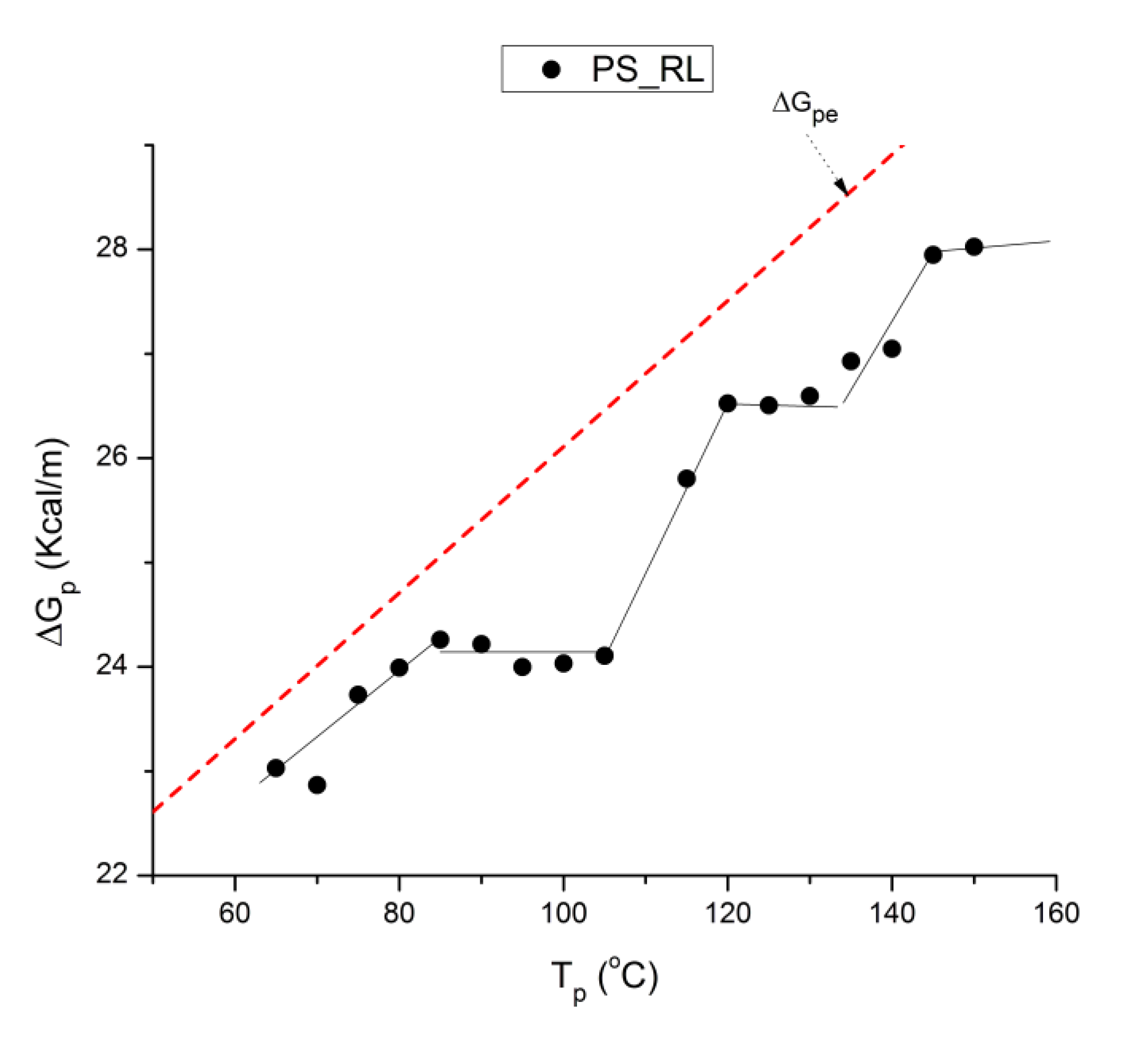
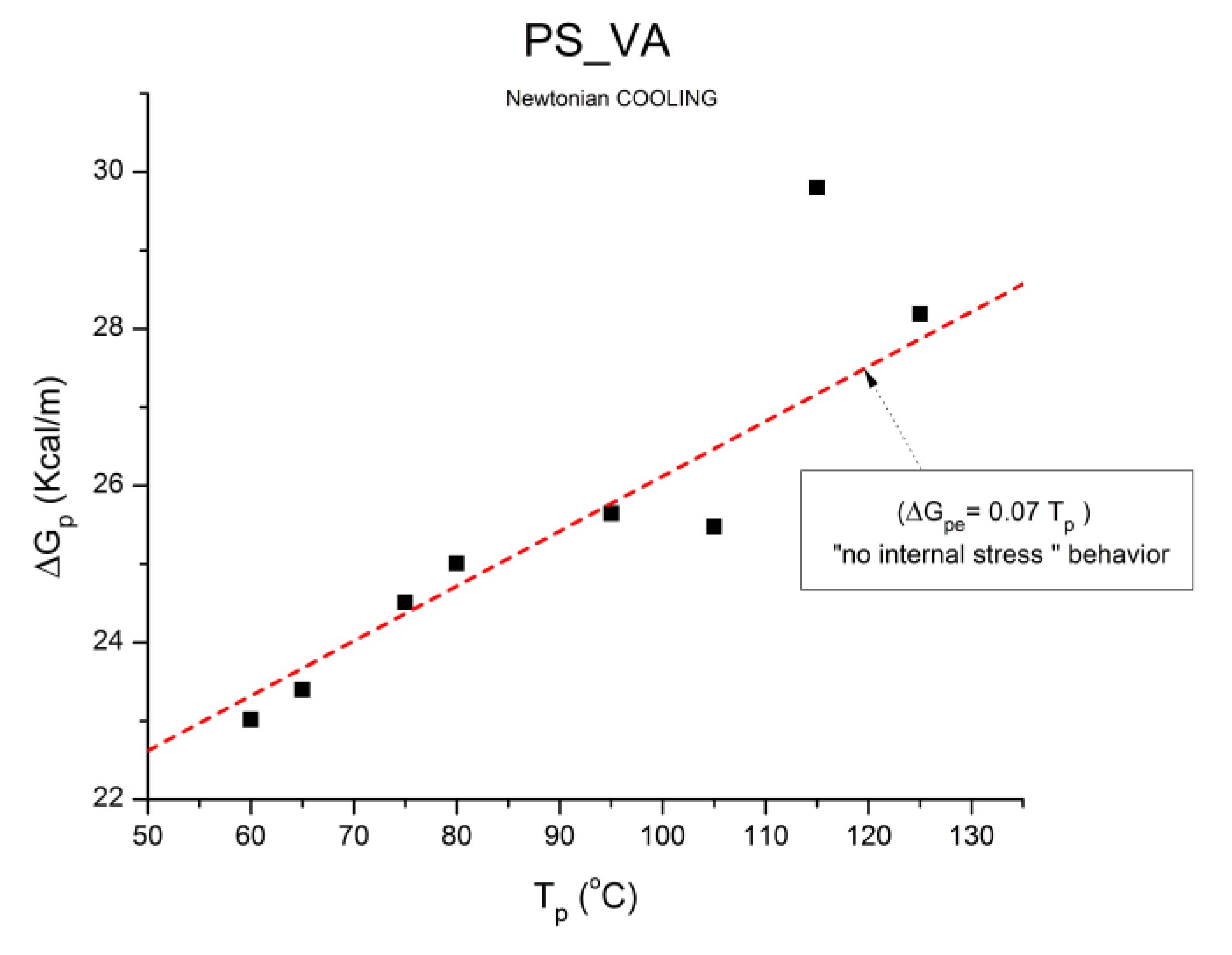
Figure 54 is a plot of ΔGp (Kcal/m) at various Tp where ΔGp is simply the calculated value of ΔG= ΔHp –T ΔSp for T= Tp. ΔG(T) is the description of the relaxation of a single Debye relaxation in the ΔG plane during the heating step in
Figure 3. Notice the difference between ΔGp and ΔGc, the latter being the value of ΔG extrapolated at the point of compensation between several relaxations. For a polymer without any singular treatment to process it, the ΔGp vs Tp behavior is typically linear and almost invariably simple: ΔGp~ 0.07 Tp (K) in Kcal/m. This reference behavior, ΔGpe, is represented by the red dash line in
Figure 54; The subscript “e” in ΔGpe refers to the pure dielectric origin of the activation of the dipoles, resulting in a local dis-equilibrium, and of its return to equilibrium during the depolarization process. The PS_RL Rheomolded sample in
Figure 54 (the black squares) has purposely been brought out of equilibrium to reveal, during the TWD process, the complex mechanisms of internal motions when the samples return to their equilibrium state during their heating or thermal annealing relaxation stages. The 3 stages of the relaxation process are indeed visible in
Figure 54. It is clear that the sample is “sustaining” to a persisting degree its initial non-equilibrium state if we compare the evolution of the squares to the dash reference line representing the equilibrium state. Yet, opening a short parenthesis, the highest temperature for Tp in
Figure 54 has not reached the TLL value of the sample, which is increased beyond 160
oC (the classical value for PS) by the mechanical treatment during cooling [
10,
11,
12].
Figure 54.
Gp vs. Tp for PS_RL. The dash red line is the expected behavior for a stable sample (with no internal stress before polarization). ΔGp = ΔHp – Tp(K)ΔSp .
Figure 54.
Gp vs. Tp for PS_RL. The dash red line is the expected behavior for a stable sample (with no internal stress before polarization). ΔGp = ΔHp – Tp(K)ΔSp .
Figure 55 is the superposition of the graphs in Figs.52 and 54. The ZIM structure of
Figure 52 is here visible as red dash lines. The blue line has the same slope as the dash line of
Figure 54 but is shifted by regression to fit the square data points. In other words, the blue line is obtained by linear regression of the squares forcing the value of the slope to equal 0.07 Kcal/m-K.
Figure 55.
This Figure is the superposition of the graphs in Figs.52 and 54. The ZIM structure of
Figure 52 is here visible as red dash lines. The blue line has the same slope as the dash line of
Figure 54 but is shifted by regression to fit the square data points. See text.
Figure 55.
This Figure is the superposition of the graphs in Figs.52 and 54. The ZIM structure of
Figure 52 is here visible as red dash lines. The blue line has the same slope as the dash line of
Figure 54 but is shifted by regression to fit the square data points. See text.
According to the 2
nd method of determination of a Tg transition from a TWD relaxation map [
16], the value of Tg is at the cross-section of the compensation line of the Z-structure pertinent to relaxation process analyzed with the ΔGp vs Tp straight line.
Figure 55 illustrates the method to determine the Tg for compensation 1 (amorphous phase 1 with Tg(-), for compensation 2 (amorphous phase 2 with Tg), and for compensation 3 (amorphous phase 3 with Tg(+). Note that, contrary to what we suggested in a previous communication (p. 495 of Ref. 5), we are affirming in this paper that Tg(-) is not associated with the Tβ transition, nor is Tg(+) associated with TLL: the visible breaks are parented to a true fragmentation of Tg, or actually of Tα, the mechanical manifestation of Tg, due to the initial conditions at the beginning of the thermal-mechanical treatment. In the Discussion (section C2) we will show that simulations with the Dual-Phase model of the interactions succeed generating positive and negative compensations, multi-compensations, super-compensations and fragmented behavior at Tg. The results below summarize our findings to describe Tg(-), Tg, and Tg(+) pursuant to
Figure 53, Eq. (13) and
Figure 55:
- -
ΔS−g = 37.42 cal/°C/m, T−g = 34.2 °C (method 1) or 72.9 oC (method 2)
- -
ΔH−g = 35.70 kcal/m
- -
ΔSg = 90.93, Tg = 90.2 °C (method 1) or 100.0 oC (method 2)
- -
ΔHg = 58.37
- -
ΔS+g = 48.72, T+g = 126.0 °C (method 1) or 129.0 oC (method 2)
- -
ΔH+g = 46.42
The only noticeable discrepancy between the two methods to calculate Tg is for Tg(-) and we have no explanation why. The two methods are compatible at 0.5 degree error for samples in a state of equilibrium [
4], an empirical rule which does not appear to apply for samples out of equilibrium due to their processing history.
We propose that these “break-transitions” of Tg, revealed by multi-compensations structuring as a Z-network, correspond to different dissipative states of the interactions between the Dual-conformers of the amorphous matter. The transition Tβ in PS, and in other amorphous polymers, is indeed a local property of the Dual-conformers, corresponding to the lower horizontal branch of the Z-structure at the scale of the elementary relaxations (lower scale). The Tg(-) break is different because it is the lower branch of a Z-structure of compensations of the Dual-conformers (higher scale), not of the Dual-conformers themselves (lower scale). The same reasoning applies to the case of TLL and Tg(+): they are equivalent but not the same because working at different scales: the TLL transition is observed in a relaxation map at the Tp temperature that corresponds to the upper horizontal branch of a Z-structure involving a lower scale. The Tg(+) break is the upper branch of a Z-structure, apparently the equivalent of TLL , but working at the higher scale level, of the compensation network. Section C2 of the Discussion and section D2 of the conclusions will explain what we really mean by “a different scale” in a Dual-Phase Dissipative context [
7].
Figure 56.
Sp vs. Tp for PS_RL.
Figure 56.
Sp vs. Tp for PS_RL.
Finally, we present a plot of ΔSp versus Tp for PS_RL in
Figure 56. For a sample in a state of internal equilibrium, there is only one Tg and the positive and negative compensations that cross at Tg (like in
Figure 53) are transposed, in a ΔSp vs Tp plot, to two hyperbolic functions on both sides of Tg sharing the same infinity axis at Tp=Tg [
16].
Figure 56 applies to a sample in non-equilibrium showing the fragmentation of Tg in 3 Tgs and the conversion of the hyperbolic functions to linear ones. There are no distinctions of behavior for either Tg(-), Tg, or Tg(+). This confirms what was hinted before that the fragmented transitions perceived below and above Tg have the same relaxation origin as Tg itself (see sections C2 and D2). Another observation in
Figure 56 is the sharp discontinuity observed between the fragmented transitions in a way rarely observed in physics except at critical transitions generated by chaotic behavior. This comment should be remembered when a Dual-Phase explanation of the fragmentation of Tg in the TWD experiments is provided in the Discussion (
Figure 68).
Figure 57.
Revised
Figure 41 considering points (4,5,6) forming a positive compensation. Also note that the intercept of lines (1,2,3,4)− and (4,5,6)+ is point 4, which is located on the ΔS = 0 horizontal line, perhaps indicating that the end of a negative compensation occurs for the Tp for which ΔS=0. Point 6 starts a new compensation for a Tp that corresponds to ΔGg = ΔGc. See text.
Let us now go back to the analysis of the slowly cooled sample PS_VA (
Figure 41). We said earlier that two negative compensations are clearly visible (
Figure 41) and that point 5 (Tp = 95 °C) was “lost”. In view of what we learned from the analysis of PS_RL we can now reexamine the situation (
Figure 57). Knowing that positive and negative compensations alternate to define the state of an amorphous phase with a Tg transition at their crossing, point 5 is in fact located on a positive compensation that linearly lines up points 4, 5 and 6. The positive compensation line is not defined with certainty in this case since we only have one intermediate point between 4 and 6 to determine its slope and intercept. Yet, the fact that 5 is exactly located on the line joining 4 and 6 gives a good probability that our assumption is correct.
We have learned how to find the values compensation points from the analysis of PS_RL above and will apply the same method below. We have calculated the following parameters:
- -
Comp(1) − : ΔSp = 3.990 ΔHp − 99.03 for Tp [60–80 °C]
- -
Comp(2) + : ΔSp = 2.624 ΔHp − 66.08 Tp [80–105 °C]
- -
Comp(3) − : ΔSp = 2.857 ΔHp − 81.93 Tp [105–125 °C]
The coordinates of the compensation points, Tc and ΔGc) expressed in the ΔG plane are found from the equation of the EE curves (above) and are compiled in
Table 5.
Notice that in the above description of PS_VA we are naming the compensations comp(1)-, comp(2)+ and comp(3)-,” since the positive compensation has been added to our initial count of 2 in
Figure 41, after we realized that point 5 was not “lost” and that a new compensation should be added to the set of the 2 negative compensations. Additionally, to match the annotations used for PS_RL, comp(3)- is actually the negative compensation line of comp(2), so its name should be changed to comp(2)-. Hence, In our new understanding of the TWD results of PS_VA, let us change the annotations to match the ones used which will make the differences between PS_VA and PS_RL appear more clearly:
- -
comp(1)- = (1,2,3,4) and the compensation point for this sub-group is C1-,
- -
com(2)+ = (4,5,6) and the compensation point for this sub-group is C2+,
- -
comp(2)- = (6,7,8) and the compensation point for this sub-group is C2-.
Figure 58 is a plot of ΔGc vs Tc , from
Table 5, using the new understanding of the compensation points.
The first difference observed between
Figure 58 for PS_VA and
Figure 48 for PS_RL is the reversal in the vertical position of the negative and positive compensation points: the negative compensations C1- and C2- are below C2+ for PS_VA, and the opposite is seen for PS_RL. This is a major difference apparently only due to their different thermo-mechanical histories. The comparison of the network of compensations for these two treatments makes it easier to realize that three additional compensations points are missing for PS_VA and would have probably become visible if we had extended the Tp range of the TWD Debye relaxations at both ends: polarizing at lower values than point 1 (Tp= 60
oC) to make C1+ visible and to higher values than point 8 (Tp=125
oC) to make C3+ and C3- visible. Using the three existing compensations points (
Figure 58) and assuming that the geometrical rules established for PS_RL remain valid for PS_VA, we can construct what the compensation network could look like for PS_VA. This extrapolated network construction is shown in
Figure 59. Amazingly, provided our assumptions are verified by new experiments with a broader range of Tp values, the network for the slowly cooled sample has become a simple parallelogram tilted upwardly, with the 3 positive compensation points aligned (red line on top), the 3 negative compensations points also aligned (blue line at the bottom) and with the parallelism of the lines passing through the positive and negative compensation points. When 3 compensations points are aligned it means that their corresponding compensations lines compensate at a single point: this is a super-compensation of the single Eyring relaxations. This same situation has been observed in Figs.45 and 56 for PS_RL. Yet, for PS_RL the coordinates of the super-compensation points of the negative and positive super-compensations are different for both axes. The fact that the network of compensations is a parallelogram for PS_VA (
Figure 58) and only a quadrilateral for PS_RL (
Figure 52) is significant and represents a characteristic of the state of non-equilibrium of the amorphous phase that can be correlated to specific thermal mechanical treatments.
The ΔHg and ΔSg values for the visible transition, Tg, at the middle of C2+ and C2- can be calculated from the intersection of the compensation lines (4,5,6) and (6,7,8): ΔHg= 68.0 Kcal/m and ΔSg=112.4 cal/m-K. The value of Tg from Eq. (13) gives 92
oC. The vertex of the pencil of line is Co (Tco= 91.78
oC, ΔGco= 26.95 Kcal/m, and therefore Tco = Tg, ΔGco= ΔGg. For the PS_VA sample, with no internal stress, Tg is exactly located at the vertex of the network of compensations. This is not true for samples which are not at equilibrium and the analysis presented in this section permits to characterize the differences.
Figure 60 below gives ΔSp vs Tp for PS_VA which should be compared to
Figure 56 for PS_RL.
The only certainty about
Figure 60 is that the last 3 points on the left (points 6,7,and 8 in
Table 1) can possibly be fitted by an hyperbola since they belong the negative branch of the Tg transition of an amorphous phase at equilibrium [
5,
16]. An hyperbolic fit is always feasible with 3 points, yet the interest is that the fit gives for the x-asymptote the vertical red line corresponding to Tp= 373 K, clearly what we expect to find for polystyrene. This is not, however, what we found for Tg using Eq. (13): we found 92
oC. On the other hand, the two points on the left side of the red line belong to an hyperbola fitting the behavior of a positive branch of a Tg transition (the asymptote for that left branch is Tg=373 K). Hence points 3,4,5,6,7 are correctly positioned with respect to a Tg transitional behavior for a sample at equilibrium. The other points (1-4) are not on that hyperbolic branch and there are possibly two reasons for this deviation. First, these points may still not be at equilibrium despite the long cooling time because the cooling sample became a glass ever since it reached 100
oC, resulting in a drastic reduction of the rate to reach equilibrium. The other possibility is that points 1-4 belong to the negative branch of the Tg(-) transition which may exist at low Tp.
Figure 61 below, ΔGp vs. Tp for PS_VA may help solve this uncertainty when it is compared to
Figure 54).
The 1
st 4 points of
Figure 54 have shifted vertically to position themselves around the “equilibrium” red dash straight line in
Figure 61 and, therefore, these 4 points belong to the negative hyperbola of Tg(-) in
Figure 60, with representative the compensation point C1- of
Figure 59.
Another comparison of PS_RL and PS_VA relates to the super-compensation coordinates. We saw for PS_VA in
Figure 59 that the red and blue lines joining the positive and the negative compensation points, respectively, were parallel to each other, separated by a distance (δΔGc= 3.494 Kcal/m and δTc= 31.1
oC ( 31.276). The equation of the positive super-compensation line is: ΔGc= 27.62+3.036 10
-3 Tc(K), and for the blue super-compensation line: ΔGc= 24.12+3.036 10
-3 Tc(K). The intercept and the slope of the super-compensation line provides the coordinates of the super-compensation points “of the lower scale correlation map”: ΔHc= intercept, ΔSc= -slope. Hence, the super-compensation coordinates for the positive and negative compensations of PS_VA can be compared to the ones shown in Figs 45 and 46 for PS_RL, respectively:
- -
PS_VA PS_RL
- -
Hsc+ = 27.62 Kcal/m Hsc+ = 23.0 Kcal/m
- -
Ssc+ = -3.04 cal/m-K Ssc+ = 0 cal/m-K
- -
Hsc- = 24.12 Kcal/m Hsc- = 17.5 Kcal/m
- -
Ssc- = -3.04 cal/m-K Ssc- = -23.0 cal/m-K
One sees that the thermo-mechanical treatment essentially lowers the enthalpy of the super-compensations, for both positive and negative compensations, the effect being stronger for the negative compensations (6.67 vs 4.62 Kcal/m). The network of compensations becomes asymmetrical pursuant to the thermo-mechanical treatment. When there was no mechanical treatment and the sample was cooled very slowly in the mold to induce a near equilibrium state for the molded sample, the network of compensations appeared symmetrical; yet the structure of the polarity of the network of compensations was reversed(upside down). Note that a confirmation of these conclusions is pending a repeat of the TWD testing of the slow cooled samples using a broader span of Tp values to validate the construction of the compensations network. Our analysis of the PS_VA results was done with only 3 compensation points and using empirical rules established from analyzing samples in non-equilibrium amorphous states. We have only presented the details of our analysis for one treated ample, PS_R, but have presented elsewhere (II.4 of [
5]) the influence of several other thermal-mechanical treatments validating the generalization of the results presented in this review: the presence of 3 scales to consider the interactions: the scale of their Debye relaxation, the scale of their compensation and the scale of the compensation of the compensations, i.e. of their super-compensation, each scale interactively coupled to the next one forming a general network of compensations.
In summary of this section B3, the Thermal-Windowing Depolarization (TWD) procedure applied to Rheomolded PS samples (compress molded under vibration) permits to quantify the influence of the thermal mechanical history on the “internal stress” incurred by the Rheomolding variables. We also show in this section B3 the power of the TWD analysis to obtain an insight into the interactive coupling relaxation mechanisms between local molecular “tags”, the dipoles, activated dielectrically. The relaxation map of these Rheomolded samples show that the deconvoluted dipole relaxations belong to a highly ordered network of compensation lines themselves compensating to a single point of the relaxation map. This “super-compensation” behavior appears to indicate a unique simple kinetic origin to the various electrical relaxation mechanisms found below Tg, at Tg, and above Tg. The phenomenon of compensation of the compensation lines of the Arrhenius relaxations generated at various Tp seems to be a key revelator of the fundamental mechanism responsible for this apparently diversified and complex behavior [
5,
16]. As we said in our objectives of this review, we will attempt to understand, in the DISCUSSION section below, the Dual-Phase gears capable of generating such an apparent simplicity, and how the interactions in the amorphous phase are modulated by the presence of compensations at different scales.
C3 Compensations, Multi-Compensations and Super-Compensations in Dual-Phase Systems Simulation
In the analysis of the TWD depolarization results we make use of compensations as a quantitative characterization tool to evaluate the interactive coupling between the Debye relaxation modes. Compensation of the Debye characteristics (ΔH, Ln τo ) means that their modes of relaxation, stimulated at various temperatures, Tp , are not independent, they are coupled. The interactive coupling is clearly visible graphically: a series of plots of log τ(T) vs. 1/T in the Arrhenius plane, or of ΔG(T) vs T in the ΔG plane [
16], when Tp varies, displays a set of spectral lines that converge to a single point, the compensation point. Hence, the compensation point coordinates appear to define the interactive coupling between the relaxation modes. When the Debye characteristics of the relaxation modes are their thermo-kinetics variables, ΔSp and ΔHp, their interactive coupling is characterized by the linearity between ΔSp and ΔHp when Tp varies. This line is the compensation line.
Most of the scientists working with TSD/TWD apply the concept of compensation to the analysis of complex TWD results, when the amorphous phase is made up of cooperative relaxation modes of different origins: for semi-crystalline polymers, for copolymers, and for blends of polymers, as well as when additives are added. In every such case the compensation characteristics of the amorphous state(s) are modified and this modification can be quantified by comparing its compensation point coordinates with a reference value. This is why the TWD characterization technique offers a unique value in the spectrum of thermal analysis instruments available to determine the properties of nonconductive materials.
Yet, beyond the practical usefulness of the use of compensations to characterize the amorphous state of non-conductive matter, the theoretical value of compensation laws is a full debate on its own. We refer to the appropriate literature for the details [43, 44, 45, and 38]. In this section, we examine the possible analogy between the compensation results obtained by TWD when Tp varies and the compensations observed in Dual-Phase systems when the variable Δe is varied in Eqs. (6-8).
The fundamental constants of the Dual-Split Kinetics model (equations (6) to (8) of Section A2) are Bo, Δm, υm, and Δe . When these constants are known, we can characterize the dynamics of this system of Bo Dual-conformers by their statistical population: their cis, gauche, and trans spatial conformation, and their b/F dissipative state, which controls the free volume in the system. The interactive coupling between the conformational states and the b/F state is described by Δx , υx , which are functions of Δm, υm, and Δe . At equilibrium, the system of interactions is stable and the b and F populations are “transparent,” i. e., undistinguishable, statistically speaking. As soon as non-equilibrium conditions occur, such as by cooling or heating, the b/F population becomes asymmetric, which is governed by a dissipative kinetics, the Split-Dual kinetics or EKNETICS as we have called it. The EKNETICS generates a Dissipative term that can be quantitatively expressed by a kinetic-like constant, kx , which varies only with T, for a given set of Δm, υm, and Δe (
Figure 27 of Section A2). As explained in Section A2, for a given value of Δe , we run simulated annealing experiments after quenching from the same temperature down to a series of five lower temperatures at which the value of (kx ) is determined from a phase plot of dNb /dt vs. Nb at t → 0.
Figure 28 shows that the temperature dependence of kx follows an Arrhenius variation, which corresponds to the linearity of Ln(kx (T)) with 1/T. From the intercept and slope of such an Arrhenius plot, we determine Ln υx and Δx , respectively, that we could hypothetically associate with an entropy and enthalpy of activation for the (b/F ↔ (c, g, t)) interactive coupling kinetics, the way we did to convert the current of depolarization into a relaxation time and determine Ln(τo ) and ΔH from the Arrhenius temperature dependence of τ(T). We repeat the simulations for a series of Δe values at constant Δm and υm. This procedure establishes the value of Ln υx and Δx for various Δe for a given set of Δm and υm. Finally, we change the values of Δm and υm and repeat the entire procedure (Note that in the TWD experiments the variables are τo and ΔH, i. e., a relaxation time and an enthalpy, whereas in the simulation υx and Δx refer to a frequency and an enthalpy. This difference results in a change of sign for the log axis variable, since 1/υx = τx ).
Figure 63 displays the influence of Δe on the kx statistics: for a given set of Δm and υm (Δm = 9250 and υm = 10
11 in
Figure 63), a compensation law is observed between Ln υx and Δx when Δe varies. The compensation between Ln υx and Δx when Δe varies is similar to the compensation between -Log τo and ΔH when Tp varies in a TWD experiment (the compensation line in a compensation search). The compensation means that the Arrhenius lines of Ln(kx ) vs. 1/T converge to a single point, the compensation point, when Δe varies. This is similar to the situation observed in a relaxation map showing the compensation of the spectral Arrhenius lines when Tp varies. As we said earlier, and is also explained in section I.2.5 of [
5] or in [
16], the coordinates of the compensation point of Ln(kx ) vs. 1/T can be determined by the slope and intercept of the corresponding compensation line in a compensation search, in our case: Ln υx vs. Δx. obtained by regression.
Figure 63.
Ln υx vs. Δx for Δm = 9,250, υm = 1011 and Δe variable.
Figure 63.
Ln υx vs. Δx for Δm = 9,250, υm = 1011 and Δe variable.
Figure 64 shows the influence of changing the value of Δm and υm on the compensation line for various Δe . Note that the variables in
Figure 64 have been “normalized,” i. e., have become (Δx − Δm) and (Ln(υx ) − Ln(υm)). When Δe varies, for a given pair of (Δm, υm), this is Δx and υx which vary. This will be important to remember when we will simulate the behavior of (ΔH, Ln(τo )) with Tp by the behavior of (Δx , Ln(1/υx )) with Δe . It should also be noted in this figure that the Δe values are rather small (from 5 to 150) with respect to Δm and that Δe decreases from left to right on the compensation lines that all pass through the origin. The origin corresponds to (Δx − Δm) = 0 and (Ln(υx ) − Ln(υm)) = 0, obtained for Δe = 0. All of these particular features are important to note to be able to correlate the effect of Tp on the Ln(τ) vs. 1/T kinetics with the effect of Δe on the Ln(kx ) vs. 1/T kinetics. In particular, we need to know if the Dual-Split model of the interactions can simulate the switch from a positive compensation law to a negative compensation law when Tp crosses the Tg of the polymer or if this results from another cause. This implies to understand how Δe and Tp are related.
It is clear in
Figure 64 that changing the values of Δm and/or υm in this low value of Δe range modifies the slope only. The inverse of the slope gives the value of Tc , the temperature of compensation for the Ln(kx ) vs. 1/T lines when Δe varies (since we have equated the gas constant to 1 in the simulations, we need to divide (1/slope) by 1.987 cal/mole if ΔHx is expressed in such units). One sees in
Figure 64 that Tc for Δm = 9,250 (square symbol) is greater than for Δm = 9,500 (the “+” symbol), at υm constant (10
11). The same slope can be obtained if we change Δm and υm simultaneously. Compare the dots (8,750, 10
12) and the “+” symbols (9,500, 10
11).
Figure 65 ,
Figure 66 and
Figure 67 show the effect of increasing Δe for these three sets of Δm and υm parameters.
Figure 65 applies to Δm = 9,500, υm = 10
11. Δe is now extended to 400 (4.21 % of Δm). We observe two compensation lines, the one passing through the origin, point O, at low values of Δe , corresponding to the “+” symbols in
Figure 64, and another straight line to cover the greater values of Δe , ending at point G in the figure. We have written the equation of the compensation lines on the graph y = αo + α1x for the larger values of Δe and y = α ′ 1 x for the low Δe values. We can express the coordinates of the compensation points of [Ln(kx ), Tc ] for these two compensation lines:
Figure 65.
Normalized compensation search of Ln(υx /υm) vs. (Δx − Δm) for Δm = 9500, υm = 1011 . Effect of varying Δe . Here Δe decreases from Δe = 400, at the left, to Δe = 5, at the far right. Notice that Δe=0 corresponds to Δx= Δm and υx= υm.
Figure 65.
Normalized compensation search of Ln(υx /υm) vs. (Δx − Δm) for Δm = 9500, υm = 1011 . Effect of varying Δe . Here Δe decreases from Δe = 400, at the left, to Δe = 5, at the far right. Notice that Δe=0 corresponds to Δx= Δm and υx= υm.
(14) Tc1 = (1/1.987α1 )
Ln(kx )c1 = αo + Ln(υm) − α1Δm
with Δe > Δeg, where Δeg is the value of Δe at point G.
(15) Tc2 = (1/1.987α ′ 1 )
Ln(kx )c2 = Ln(υm) − α ′ 1 Δm
with Δe < Δeg.
Could the two compensation lines of
Figure 65 simulate the change of behavior at Tg for an amorphous phase analyzed by TWD? Let us consider the experimental evidence first: for a Debye relaxation map, scanning Tp from a low value below Tg , crossing Tg , and above Tg , we go from a positive compensation to a negative compensation, meaning that the value of ΔHp , the slope of the Arrhenius line, increases first with Tp , passes through a maximum value at Tg , and then decreases towards a minimum value. This maximum of ΔHp describes the typical response of an amorphous phase submitted to a voltage field stimulation according to the thermal-windowing protocol (
Figure 3). Now, assuming that we can simulate the effect of Tp on the depolarization kinetics by a change of Δe on the kx relaxation kinetics, we can formulate and test the hypothesis that the compensation line below point G in
Figure 65, corresponding to the higher values of Δe , simulates the Tp < Tg positive compensation and that the compensation line above point G, corresponding to lower and vanishing values of Δe , simulates the negative compensation. This would only occur if:
(16a) Tc2 < Tc1 and
(16b) Ln(kx )c2 > Ln(kx )c1 (3.3b)
The first requirement is met since α ′ 1 > α1 in
Figure 65, which, plugged into equations (14) and (15), means that (16a) is true. The second requirement, (16b), will be met if and only if:
(17) Ln(kx)c2 = {Ln(υm) − α ′ 1 Δm} > Ln(kx )c1 = {αo + Ln(υm) − α1Δm}
where the expressions of Ln(kx )c1 and Ln(kx )c2 are brought in from (14) and (15), respectively. Equation (17) simplifies to:
(18) Ln(υm/υxg) + α1 (Δxg − Δm) < (α ′ 1 − α1 )Δm
where υxg and Δxg are the values of υx and Δx at point G, at which Δe = Δeg. Hence, we must demonstrate that:
(19) Ln(υm/υxg) < α ′ 1 Δm − α1Δxg
But at point G, we also have:
(20) Ln(υxg/υm) = α ′ 1 (Δxg − Δm) which is the transposition of y = α ′ 1 x
Finally, the second requirement in equation (16b) resumes to test if equation (21) is true:
(21) α ′ 1 (Δm − Δxg) < α ′ 1 Δm − α1Δxg
Equation (21) simplifies to:
(22a) −α ′ 1 Δxg < −α1Δxg
or
(22b) α ′ 1 > α1
which is always true when Tc2 < Tc1.
In summary, the two conditions (16a) and (16b) are verified and we could conclude that
Figure 65 is the correct representation of the positive and negative compensations observed for describing interactive coupling in the amorphous phase of a homopolymer across its Tg. This analogy implies that Δe decreases as Tp increases, which is observed in
Figure 65 since Δe decreases from left to right.
But there is one remaining question to consider: even if this solution seems to work, is it the only plausible solution? In other words, is the solution offered by
Figure 65 the only possible explanation for the switchover at Tg from a positive to a negative compensation? Here are a few good reasons to remain cautious:
1. The simulation in
Figure 65 is not exactly a simulation of the TWD experiment (we will get back to that point). In particular, the depolarization stage in a TWD experiment is obtained under a thermal temperature ramp at constant rate. This is not the case for the Dual-Split model simulations which are done under isothermal conditions.
2. If equations (16) to (21) were truly simulating the TWD two-compensation split at Tg , point G in
Figure 65 would correspond to the Tg of the polymer system of interactions. At this point Δe = Δeg, which can be obtained from the simulation data, and the values of Δx and Ln υx are those at point G. The crossing of the positive and the negative compensations in an amorphous polymer occurs at Tp = Tg , defining the characteristics of the Z-line, the line joining the two compensation points. But, the existence and the position of the break in
Figure 65 is determined by the choice of the values of Δm and υm. As we will see, for certain pairs of Δm and υm, the break observed at point G in
Figure 65 is not observed (see
Figure 67 discussed later). This could, of course, simply mean that the choice of Δm and υm to simulate polymers should be restricted to those values that display a break conform to
Figure 65 in their compensation search when Δe varies. The fact that the choice of Δm and υm is not unlimited, but rather should correspond to some criteria to meet the requirements that they simulate polymers, is, indeed, a reasonable proposition that we believe is true, regardless of the issue considered here.
3. But the fact that we need to assign a certain value of Δe equal to Δeg, the value of Δe when Tp = Tg, faces various objections. The first objection is that Tg is a kinetic phenomenon observed whether a voltage field is applied or not. In Section A2, we attribute to kinetic reasons the freezing of the statistical populations at low temperatures. This occurs for all values of Δe , not just a specific one. The second objection is that we attribute the break in
Figure 65 to the interference on the kinetics of kx of the coupling between Δe and (Δm, υm): this is what we mean by interactive coupling between the conformational states and free volume (the b/F state). The coupling is more prominent at large values of Δe , for Δe > Δeg in
Figure 65, and simplifies to a pure influence of Δe alone at lower values of Δe , vanishing to 0. This has nothing to do with a Tg transition which shows up for all values of Δe . Besides, in the simulations, the value of Δe is constant during cooling or heating; it is not a function of T. Even if, in our explanation of the compensation of ΔH and ln τo , it has been said that the value of Tp during the polarization stage fixes the value of Δe , this value remains constant during the simulation of the cooling and depolarization stages. It is possible, obviously, to change this assumption in the simulations and make Δe a function of T, but this was not the case in the simulations that led to
Figure 65.
Our conclusion is that despite the remarkable and simple explanation provided by the break in
Figure 65, we need to find another explanation for the sharp change of the compensation slope and intercept at Tg that results in the positive followed by a negative compensation across Tg. We have found such an explanation and it is not based on the change of slope in
Figure 65, it has to do with “grid-shifting,” which is not detailed in this review but in I.3.4.5 of [
5]. Grid-Shifting essentially says that there are 3 rheological temperature “scaling ranges” for the internal mobility in amorphous polymers [
11,
12] and that the transfer function of Eq. (22) below is affected when the polarization temperature, Tp, is located in either one of these 3 ranges. For Tg <Tp < Tg+25, the kinetics of molecular motion wakes up the elastic dissipative wave that starts to un-freeze, move around and delocalize the (b/F) pockets of free volume around the b-grains which remained frozen for Tp below Tg. This reorganization of the pockets of free volume is responsible for a change of the polarization nature in this temperature range above Tg, changing from electronic and atomic polarization to orientation polarization: this modifies the polarization efficiency, i.e. the ability to modify Δe at Tp. As we will see with respect to
Figure 67,
Figure 68,
Figure 69 and
Figure 70, a large initial value of Δe (E, Tp ), relative to its equilibrium value, may be present in the sample at Tp, during the polarizing stage, as frozen-in internal stress was induced by a mechanical treatment during the processing of the TWD sample, and such an initial Δe value present at Tp, could change drastically the depolarization behavior such as the slope and the intercept of the compensation in
Figure 66.
In the equations of the Dual-Split model (EKNETICS), the dynamics of the interactive coupling between the Dual-conformers is characterized by the dissipative thermo-kinetic values, Δx and ln υx, which, we saw, depends on the value of Δe. If we want to apply this model to the dynamics of the polarization and depolarization of the dipoles, aka the activated or deactivated Dual-conformers, we need to figure out or assume the coupling equation between the voltage field, E, the polarization temperature, Tp and Δe: Δe(Tp, E). Equation (22) below, is formulated from considerations of both the Dual-Phase model and the thermos-kinetics of the dipoles by TSD/TWD:
Point O, in
Figure 65, can be associated with a temperature Tx of the polymer system of interactions for which Δe = 0. We assume that Tx is the thermodynamic value of TLL. In other words, Tx is the Tp value corresponding to Δe = 0. We still need to understand the physical meaning of Tx . At the origin O, x = y = 0 and thus υx = υm and Δx = Δm. Therefore, this state does not generate asymmetric b/F statistics, which is our definition of TLL. We view Tx as the thermodynamic (rate-independent) transposition of TLL that can only be experimentally measured by extrapolation of TLL at zero rate. Regarding the TLL transition, we have made previous statements that it is the temperature of “superposition” of the b and F states; borrowing an expression from quantum mechanics, we have called it “the temperature at which the b and F states become ‘transparent’ or ‘undistinguishable’.” Yet, in the Dual-Split statistics, a system of interactions at equilibrium is de fined by three fundamental constants, Δm, υm, and Δeo, not simply Δm and υm. We, therefore, suggest that TLL is the temperature at which Δe (Tp ) = Δeo, which provides a dynamic character to the “superposition” transition. By combining the statements above regarding the value of Δe at Tg , TLL, and Tx , we can tentatively conclude that Δe varies with Tp and the voltage field E such as:
(22) Δe (E, Tp ) = Δeo + kF(α, μ,N) E (TLL − Tp ) TLL
where E is the normalized voltage field (V/m), F is a transfer function affecting the efficiency of the modification of Δe, α, μ and N are polarization Debye parameters expressed in a modified generalization of the Clausius-Mosetti formulation of the dielectric constant ( Eq. 3.20 p. 245 of [
5]) and k is a scaling constant.
(23) At Tp = TLL Δe = Δeo
Δe = 0 for Tp = Tx
Tx is the thermodynamic value of TLL
Δeo is also the value of Δe when the material is not dielectrically stimulated (E = 0). Note that F(α, μ,N) in equation (22) is a transfer function between the macroscopic and the molecular world, which, for the present purpose, does not need to be discussed, but can be derived from the expression of the dielectric constant, ε, as a function of the total dipole moment, permanent and induced, and the number of dipoles, N (Eq. 3.20, p.245 of [
7]). Equation (22) can be rewritten as a function of Δeg:
(24) Δe (E, Tp ) = Δeo + (Δeg − Δeo) (TLL − Tp ) (TLL − Tg ) with:
(25) Δeg = Δe (E, Tg ) = Δeo + kF(α, μ,N) E (TLL − Tg ) TLL
Equation (22) is assumed to couple the electrical field effect and the temperature effect, using the framework of the Dual-Phase concept to define interactions in dielectric materials: in other words, it is assumed that these two effects are not separable but coupled ; furthermore, since TLL and Tg are rate dependent and thus subject to the thermal history, Δe(E,Tp) is also function of time for samples out of equilibrium and function of the annealing parameters. The true simulation of the TWD polarization and depolarization stages, using the Bucci equations has been covered elsewhere (Eqs. (1.21)–(1.24) of I.1 of [
5], but is not what is simulated in Section A2 and in
Figure 61,
Figure 62,
Figure 63,
Figure 64,
Figure 65,
Figure 66,
Figure 67,
Figure 68,
Figure 69 and
Figure 70, which reports the effect of Δe on Δx and υx for an
isothermal relaxation taking place to determine Δx and Ln(υx ) at various Δe. In other words, the TWD relaxation protocol is different from the Dual-conformers relaxation protocole’
When Δm and υm take another set of constant values, the aspect of the normalized compensation search shown in
Figure 65 presents notable changes, as evidenced by
Figure 66 and
Figure 67.
Figure 66 applies to the system: Δm = 8,750 and υm = 10
12 and
Figure 67 to the system: Δm = 9,250 and υm = 10
11 already analyzed in
Figure 63, but now presented with an extended range of Δe values (from 5 to 900).
Figure 66.
Influence of Δe on Δx and Ln υx using the normalized variables .This is the same graph as in
Figure 65, except that Δm = 8,750 and υm = 10
12. The point (x) for (Δx − Δm) = -268 appears to be off the line. See text.
Figure 66.
Influence of Δe on Δx and Ln υx using the normalized variables .This is the same graph as in
Figure 65, except that Δm = 8,750 and υm = 10
12. The point (x) for (Δx − Δm) = -268 appears to be off the line. See text.
Figure 67.
Similar to
Figure 65 except that Δm= 9250 and Δe ranges from 900 to 5 as the index of the points continuously decreases from point #12 to point #1 in
Table 6. What may appear chaotic can be considered a network of interlaced positive and negative compensation lines (
Figure 68) for Ln(υx) vs. Δx.
Figure 66 provides the same information as
Figure 65: the existence of two compensation lines defined by points G and O and the slopes α1 and α ′1 such that α ′1 > α1 . Again, the simulation results for a different set of Δm and υm values corresponds to positive and negative compensations for Ln(kx ) vs. 1/T. The differences bear on the relative positions of the compensation lines, their intercept defining Δeg, and the relative magnitude of Tc1 and Tc2. The other observable difference is the last point on the left corresponding to Δe = 400 and (Δx − Δm) = -260, on the higher Δe side of the y = αo + α1 x compensation line. This point is totally off the compensation line, as if it was due to an error. But the simulation for this particular Δe is entirely similar to the other simulations, at lower values of Δe , with the same regression accuracy in the determination of the values of kx (T) to find the corresponding Δx , Ln υx . Thus this point is not due to a simulation error; it is real. We further analyze this apparently erratic phenomenon in
Figure 67. As we said, this figure explores the same Δm, υm settings as in
Figure 63, yet with a much broader range of Δe values: 12 values ranging from Δe = 5 to Δe = 900.
Table 6 provides the results of the simulation.
Figure 67 is a normalized compensation search apparently showing one compensation line only: for points 1–6 (the other points are connected by dash lines). The points are tagged by their row number listed in the first column of
Table 6. They are sorted by increasing Δe values. The overall view of the effect of an increase of Δe for these Δm, υm settings is that beyond a certain value, say corresponding to the end of the compensation line (1-6), the dissipative system of Δx, Ln(υx) values becomes chaotic in appearance. We have drawn dashed lines linking the successive points, following a continuous increase of Δe, and we observe the typical response of scattered disorder. For this particular set of values for Δm and υm, and for Δe between 0 and say 400, we find a compensation line (1-6) susceptible to simulate a positive TWD compensation line in a compensation search of -Ln τo vs ΔH. Beyond that value of Δe, which is a function of the choice of Δm and υm, we imagine in
Figure 68 a certain order of the chaos by drawing a series of alternative positive and negative compensations, identified by the direction of the arrow connecting adjacent points. For instance in
Figure 68, the 1
st positive compensation line (1-6) would not end at point 6 but at the intersection of line (1-6) and line (7-8), with the direction of the arrow going down for (1-6) and up for (7-8).
Figure 68 uses the same data as in
Figure 67 (
Table 6), replotted as Ln υx vs. Δx (without the normalization of the axes by υm, Δm) to show the analogy with the compensation search of -Ln τo vs ΔH (or ΔSp vs ΔHp in the Eyring plane. In
Figure 68, we have drawn three black lines with an arrow pointing down and two red lines with arrows pointing up. The arrows follow the tendency for the y-variable, Δx, to decrease or increase within a range. The ranges are determined arbitrarily since the lines only join two points (with the exception of the first range which has six points). It would, indeed, be quite useful, in a complementary research project, to increase the number of Δe values to resolve the definition of the ranges in
Figure 68 (for instance Δe= 472.5, 550, 625, 675, 733, 766, 833, and 866). But the main idea in this section of this review is to suggest that there is an analogy between the compensation of the -Ln(τo) vs 1/T Arrhenius lines seen for the TWD depolarization behavior when Tp varies and the Ln(kx ) vs. 1/T relaxation results of the EKNETICS when Δe varies at Δm and υm constant. The analogy associates the roles played by Tp and Δe in their respective relaxation processes, which may have consequences on our understanding of what is actually deconvoluting in a Thermal Windowing procedure (see Section C4).
Figure 68.
Same compensation search as in
Figure 67, without the normalization of the axes by Δm, υm to make the analogy with -Ln τo vs ΔH in depolarization compensation search at various Tp more apparent. Note that Δe increases continuously between (point #1: Δe = 5 and point #12: Δe = 900). One can define positive compensations (black arrows pointing downward, showing a decrease of Δx as Δe increases) and negative compensations (red arrows pointing upward, showing an increase of Δx as Δe increases).
Figure 69.
Variation of Ln(υx /υm), at υm and Δm constant, against Δe for the data of
Figure 67 (
Table 6).
Figure 69.
Variation of Ln(υx /υm), at υm and Δm constant, against Δe for the data of
Figure 67 (
Table 6).
Figure 70.
Variation of (Δx − Δm), at Δm constant, against Δe for the data of
Figure 67 (
Table 6).
Figure 70.
Variation of (Δx − Δm), at Δm constant, against Δe for the data of
Figure 67 (
Table 6).
The apparent multi-compensations structure imagined in
Figure 68 to explain the chaos observed for large values of Δe in
Figure 67 raises another analogy with a TWD behavior seen for samples put out of equilibrium by “strong” processing conditions (Rheomolding treatments) before testing them by TWD. For instance in
Figure 68, as Δe decreases continuously from a high value, the “positive” lines (11–12, 8–9, and 1–6,) appear to compensate into a super-compensation, while the interlaced “negative” lines (10–11 and 3–8) compensate into another super-compensation; the analogy is with Figs 45 and 46, respectively, for Rheomolded sample PS_RL.
Figure 69 and
Figure 70 present another angle to reveal the possible structure of Δx and Ln υx at higher values of Δe . These figures plot the variation of the normalized data, (Ln υx/υm) and (Δx - Δm ), against Δe:
Figure 69 and
Figure 70, respectively. The first observation is that Δx or Ln(υx ) decreases when Δe increases in range 1 [points 1–6]; this correlation is the same for the other positive compensations, but is the opposite for the negative compensations: (Δx or Ln(υx ) increases when Δe increases. A second observation is that in range 1 a quadratic equation can be used to fit the Δe dependence of either Ln υx or Δx . This permits to evaluate the value of Δe that ends the first range or starts the second range: we find Δe = 445 with Δx= 8,835 and Ln υx = 24.6. The third observation is that there seems to be a periodic oscillation of the ups and downs for adjacent ranges, with the down values possibly aligned on straight horizontal line in the case of (Δx – Δm) in
Figure 70. These observations are
possibly the analogs of what was expressed in Section B3, Figs.41, 45, and 46 for instance, regarding the relaxation map for a classical amorphous polymer, polystyrene, which could be fragmented into separate groups, each with a characteristic compensation point; the number and sign of these multi-compensations depended on the thermo-mechanical history on cooling. The network of compensations (
Figure 50,
Figure 51 and
Figure 52) revealed a simple relationship between the various compensation lines in the compensation search plane, from 50 °C below to approximately 60 °C above Tg . We concluded that the relaxation process described by the individual relaxation modes, i. e., occurring below Tg , at Tg , and above Tg, was correlated as a structure of compensations and super-compensations.
Now, the analogy between these two types of relaxations, both complex and difficult to analyze: the Dual-Phase relaxation when Δe varies “widely” and the TWD relaxation of “widely” out of equilibrium samples when Tp varies, appears to be strikingly confirmed. We just need to qualify what “widely” means for the TWD results and the Dual-Phase dynamics simulations.
Consider
Figure 68,
Figure 69 and
Figure 70, in particular
Figure 68 in the one end, and Figs, 45, 46 and 57 in the other end. Could it be suggested that the network of compensations observed for the TWD thermokinetics of these out of equilibrium samples be generated
by a combination of two effects on the value of Δe of the Dual-Phase system simulating the dynamics of the interactions when the sample is relaxing to return to its equilibrium state? The two effects that modify Δe are:
1. the thermomechanical history during the processing of the sample;
2. the thermal dielectric history during its TWD characterization.
The coupling of both of these effects the value of Δe (E, Tp ,t) of Eq. (22) in a way that brings its value in the range that appears chaotic, but is in fact structured, as suggested by
Figure 68. As the TWD sample anneals at different stages of the TWD protocol, for instance as Tp is raised or during the depolarization at Td during a time td, and the heating stage at constant rate, then the value of Δe(E,Tp) decreases, passing through the different values of Δx, Ln υx from left to right in
Figure 68, revealing the multi-compensation structure of Ln υx vs. Δx along the way.
Our tentative conclusion for Section C3, provided our analogy assumption is founded, is that the TWD characterization technique reveals the dissipative mechanisms of structuration of the interactions that we have assumed are the basic assumptions controlling the behavior of polymers. In such a case, the TSD/TWD method should, somehow, lead to the determination of the fundamental parameters of the statistical model of polymer interactions introduced in Section A2. The value of Δe is equal to Δeo at equilibrium, but we cannot measure it directly, except at T= TLL. The value of υm and Δm are unknown , especially since what we are measuring are υx and Δx, except at Tx, the thermodynamic value of TLL, where Δe=0 and υm= υx and Δm= Δm. In order to find Tx we must modify the state of non-equilibrium of the amorphous phase by mechanical means and/or by di-electrical means in order to access it by extrapolation.
D CONCLUSIONS.
This communication reviews the comprehension of “interactive coupling” between molecular motions in AMORPHOUS polymers using data generated by Thermally stimulated depolarization (TSD) and Thermal-Windowing Deconvolution (TWD), analyzed either “classically”, pursuant to work published on the subject [
1,
2,
3,
6] or “un-conventionally”, using the language of the Dual-Phase model of polymer interactions {10-13]. TSD and TWD are two characterization methods that involve thermally inducing polarization in dielectric samples by a voltage field and subsequently follow its depolarization by heating the sample at constant. TSD / TWD provide a powerful way to quantify the “thermo-kinetic” state of amorphous matter by studying the local and cooperative relaxations occurring during the depolarization stage. The understanding of the amorphous state of matter is, in our opinion, essential to understand the glass transition, molecular motions in the rubbery and molten states, and even the fundamental mechanisms leading to crystallization from the amorphous state.
This review summarizes the fundamentals of this dielectric characterization technique using the “classical approach language”:
- -
the polarization and the depolarization stages, the description of the current of discharge by the Bucci’s equations [
14,
15]; the filtering of the spectrum of relaxations to isolate various elementary Debye relaxation peaks and the compensation of the Debye relaxation times deconvoluted by “Thermal-Windowing”.
- -
the origin of the dipole formation, induced or permanent dipoles, the origin of the Wagner space charges,
- -
the observation of the Tg,ρ peak just above Tg and of the TLL manifestation, spectroscopic nature in a relaxation map, the description of their compensation and, for certain specimens (Rheomolded) of their multi-compensations and super-compensations (the compensation of the compensation lines themselves).
This review also introduces the “language” of a new physics of polymer interactions [
10,
11,
12,
13], the Dual-Phase theory, and applies it to simulate the relaxation of a closed system of dissipative Dual-conformers that are assumed to be the statistical basic units that interactively couple to explain the viscoelastic properties of polymers. We use the language of this “un-conventional” statistics (with the introduction of a dissipative term in the energy equation) to describe and understand the dielectric properties of amorphous polymers. It is assumed that the Dual-conformers have been polarized to generate the dipoles and that the space charges localize at the space around the b-grains (F-conformers). The simulations explain the dynamics of the dissipative system of dipoles on cooling, heating and relaxation and show, for instance, how cooling at constant rate brings the system out of equilibrium , in a way different from a non-dissipative system. The temperature at which the system starts to become dissipative (on cooling) or ceases to be dissipative (on heating) is assimilated to the TLL transition easily detectable by TSD and TWD manifestations. Also the presence of the F-conformers (attributed to the Free volume around the b-grains), attracts and localizes the Wagner space charges in the amorphous structure and explains the presence of the Tg,ρ peak in TSD experiments. The dissipative thermo-kinetics parameters, υx and Δx, which are self-generated by the inducement of the non-equilibrium states are fundamental parameters of this new kinetics (the EKNETICS), that are associated by analogy to the thermo-kinetic parameters, 1/τo and ΔH, extracted from the analysis of the relaxation map in TWD experiments. The analogy between the simulated relaxation dynamics of the Dual-conformer and the relaxation dynamics of the dipoles during the depolarization stage explains the structuring of their interactive coupling as positive and negative compensations across the Tg transition. The super-network of compensation structures observed for the Rheomolded PS samples (brought out of equilibrium by mechanical means) can also be simulated. Interestingly, a relaxation map that appeared complex and incomprehensible at first, in
Figure 45 and
Figure 46, turned out to have a very simple Dual-Phase explanation to comprehend it (
Figure 68). This apparent successful theoretical break through to explain compensations and super-compensations may be regarded as a sort of validation of the power of the TSD/TWD thermal analysis technique to measure-up the amorphous state of electrets [
5]; and , on the theoretical side, it may also provide the proof of the benefits of using the Dual-Phase statistics to simulate the properties of polymers, including to provide a coherent interpretation of the TLL and Tgρ manifestations.
There is also another dimension to this review: we argued in section C4.3 that our understanding of compensations in the TWD experiments based on the analogy with compensations in the Dual-Phase simulations challenged the “classical” physical meaning of Thermal Windowing itself (sometimes designated “Thermal-Sampling”); the Dual-Phase approach suggests that Thermal-Windowing reflects the deconvolution of the Dual-Split complexity of the interactions, with Δe decreasing towards Δeo as Tp varies (
Figure 68), which contradicts the classical interpretation of Thermal-Windowing as the deconvolution of global peaks into elementary Debye peaks. Likewise, the classical “local order” explanation of the TLL manifestations (TSD in
Figure 36, TWD in
Figure 11 (ΔSp=0)) and of the Tg,ρ peak (
Figure 30,
Figure 31) is not consensual among the protagonist users of the TSD/TWD technology [
1,
2,
3,
6]. The Lacabanne’s school interpretation of the compensation of ΔH and Ln(τo) [
6], was challenged by Sauer and Moura Ramos [
38] who raised the issue whether compensation had a real physical meaning. The Dual-Phase response to that question validates the question of these authors by providing a new interpretation of the compensations than the classical answer. However, the questioning of the core interpretation of Thermal-Windowing was the good bargain used by the adepts of the current paradigm to discredit the reality of TLL, a transition notably more visible by TSD/TWD than by other technologies [
36,
37]. There is no theoretical resonance in the framework of the current paradigm of polymer physics for TLL and Tg,ρ [
12,
13]. The backers of the molecular dynamic models of polymer physics (the gate keepers of the current paradigm) rightfully recognize the existential threat to their paradigm of the existence of the TLL transitions, and claim that it is an experimental “artifact”[
36,
37]. Finally, the question of the negative compensations found for Tp > Tg and of the Z-structure at Tg (Fig, 11) is never mentioned by neither the protagonists of the TSD/TWD, (as if it was not a reality) nor by the gate keepers of the current paradigm. who prefer to ignore all the facts that they cannot designate “artifacts”. Hence, It seems clear, in this context of theoretical questioning [
36,
37,
38], why the TSD/TWD methodology has only been partially adopted as a powerful characterization technique. For instance,
Yet, the recognition of TLL is essential, in our view [
10,
11,
12,
13,
14], for the understanding of the dissipative nature of polymers pursuant to the Dual-Phase theory (
Figure 62) and also to comprehend the logic behind the “disentanglement” processing technologies to improve the fluidity of melts (Rheo-Fluidification) and pellets (“Sustained-Orientation”) benefitting their final properties [
10].
In summary, we believe that a broader recognition of the merits of TSD/TWD in Thermal Analysis requires the correct interpretation of the TLL transition and of Tg,ρ and, moreover, of the reality of compensations [
38]. This implies a clear and straightforward presentation of the facts regarding their experimental manifestations and a solid theoretical explanation of how their physical presence can be integrated with the rest of the properties of polymers. This requires, in our opinion, to make advances in two fronts: 1. present a new understanding of the TSD /TWD results (this is the objective of this review) and 2. make the current paradigm of polymer physics (molecular dynamics) obsolete by providing a different explanation of the experimental facts by the Dual-Phase theoretical language. The molecular dynamic models, despite their many successes, are presently facing too many deficiencies and continue to ignore them {12,13]. The experimental evidence for which the current paradigm of polymer physics is called deficient is explained in several papers [
10,
11,
12,
13] and also, implicitly, in this review of the TSD/TWD results. The deficiency of the molecular dynamic models regards various aspects of the visco-elasticity of the melt: in rheology, the non-linearity of shear-thinning [
10,
11] and the misconception of entanglements [
12]; in processing, the incapability to comprehend “sustained-orientation” by Rheo-Fluidification [
10,
11,
12,
13]; and, in this review and in [
5], the lack of consideration to take into consideration the existence of fundamental transitional behavior observed by TSD/TWD: the TLL transition and the Tg,ρ peak. The alternative Dual-Phase interpretation for those same experimental facts has been published for the last 10 years [
5,
8,
10,
11,
12,
17] and has yet received no contradiction/interest.
In our view, “Dual-conformers,” the constituents of the macromolecules, gather into statistical systems which go beyond belonging to individual macromolecules. A conformer is shown in
Figure 13, duplicated from reference [
19]. The macromolecules themselves represent a chain of “covalent conformers” put together as an entity. The problem is to determine whether the chain properties, derived from its statistics, control entirely the dynamics of the collection of chains making up a polymer. This is what has been assumed by all the other theories, and this is what the Dual-Split Kinetics and the Grain-Field Statistics challenge. In our opinion, this is a key issue: the currently established theoretical models of the interactions in polymers are based on “chain dynamics” statistics. In rheology, for instance, the Rouse and reptation models are dominant for M < Mc and M > Mc , respectively [
11]. The conclusion obtained from the present work, based on the Grain-Field Statistics of the interactions, is that the application of macromolecular (chain) dynamic models could only be justified for conditions of use that position its temperature above the TLL transition (T > TLL). The big problem is that the existence of TLL is not even recognized by these macromolecular dynamic models. Below TLL, the free energy of the collection of chains assembled as a polymer is not equal to the scaled-up free energy of a macromolecule embedded in a mean field created by the influence of the other macromolecules. Besides, the temperature TLL is itself a function of the dynamics of the experiment and the chain characteristics. The Dual-Phase model of polymer interactions does not require, in its hypotheses and derivations, a description of the changes which occur to the individual macromolecules. The dynamic statistical systems dealt with in this model, used to determine the free energy and its structure (enthalpy and entropy), are not the macromolecules. However, the fact that macromolecules compose the basic structure is essential to understand the basis of our new Dual-Phase statistics and to explain “entanglements,” for which the Dual-Phase model provides a completely different interpretation than the ones offered by the conventional macromolecular dynamic models [
11,
19]. A “Dual-conformer” is not the same as a “free conformer” (
Figure 13), defined from the monomer repeat unit involved in the polymerization process. Its interaction to other conformers by covalent bonding modifies the conformational potential energy of a free conformer, and this governs the statistical properties of a “free chain. When dealing with a collection of chains put together, our approach differs from the classical one. Dual-Conformers belong to two types of sets: they belong to macromolecules, which link them via covalent forces, as we just said, and they belong to the grand ensemble of conformers which are linked by inter-intra molecular forces, van der Waals, dipole-dipole, and electrostatic interactions which affect and define the viscous medium. That duality is intrinsic to conformers, which we call the “dual-conformers” to mark this specificity. The potential energy of a dual-conformer is different from the potential energy of a conformer part of a free chain. To simplify, one could view the difference between our statistical model and the classical model to describe the properties of polymers as follows: according to the classical views, the statistical systems are the macromolecules, i. e., a network of chains; the properties of the chains are disturbed by the presence of other chains and by the external conditions (temperature, stress tensor, electric field, etc.). The classical definition of the statistical system as the macromolecule contrasts with our approach whereby the statistical systems are the “dual-conformers,” not the macromolecules. The interactive coupling between the dual-conformers is defined by a new field of statistics, the Grain-Field Statistics that explores the correlation between the local conformational property of the dual-conformers and their collective behavior as a dissipative network.
Figure 1.
Description of the steps involved in a TSD experiment (polarization, cooling, annealing, heating) resulting in the output (a depolarization current vs temperature) by thermal stimulation.
Figure 1.
Description of the steps involved in a TSD experiment (polarization, cooling, annealing, heating) resulting in the output (a depolarization current vs temperature) by thermal stimulation.
Figure 2a.
Depolarization current vs temperature during the thermal stimulation heating stage of Polyamide 12.
Figure 2a.
Depolarization current vs temperature during the thermal stimulation heating stage of Polyamide 12.
Figure 2b.
Depolarization current vs temperature during the thermal stimulation heating stage for a polarization temperature near the -transition of an amorphous polymer.
Figure 2b.
Depolarization current vs temperature during the thermal stimulation heating stage for a polarization temperature near the -transition of an amorphous polymer.
Figure 3.
Description of the steps involved in a TWD experiment to thermally deconvolute a global TSD peak into its elementary Debye components and determine the interactive coupling between the relaxation modes.
Figure 3.
Description of the steps involved in a TWD experiment to thermally deconvolute a global TSD peak into its elementary Debye components and determine the interactive coupling between the relaxation modes.
Figure 4.
Current of depolarization vs T for a TWD experiment. The polymer is PMMA.
Figure 4.
Current of depolarization vs T for a TWD experiment. The polymer is PMMA.
Figure 5.
Effect of changing the polarization temperature Tp in a TWD experiment, indicated by the arrow, on the current of depolarization vs T plot.
Figure 5.
Effect of changing the polarization temperature Tp in a TWD experiment, indicated by the arrow, on the current of depolarization vs T plot.
Figure 6.
Conversion of the output in
Figure 4 to an Arrhenius spectral line. The bottom axis is the Arrhenius scale, 1/T (K), in descending numbers; the top axis is the temperature in
oC. The y-axis is the log of the relaxation time for the mode isolated by TWD at Tp.
Figure 6.
Conversion of the output in
Figure 4 to an Arrhenius spectral line. The bottom axis is the Arrhenius scale, 1/T (K), in descending numbers; the top axis is the temperature in
oC. The y-axis is the log of the relaxation time for the mode isolated by TWD at Tp.
Figure 7.
Relaxation map in the Arrhenius plane of all the relaxation modes isolated by TWD at various Tp, as shown in
Figure 5.
Figure 7.
Relaxation map in the Arrhenius plane of all the relaxation modes isolated by TWD at various Tp, as shown in
Figure 5.
Figure 8.
Illustration of the effect of various mechanical treatments of the melt during molding on the aspect of the relaxation map obtained by TWD of the glasses produced.
Figure 8.
Illustration of the effect of various mechanical treatments of the melt during molding on the aspect of the relaxation map obtained by TWD of the glasses produced.
Figure 9.
Response of a dielectric material to an ac voltage field. A Cole-Cole plot (top) consists of a plot of ε”(f) vs ε’(f) at a given T; A frequency map is shown at the bottom for ε”(f,T). Such plots can be calculated from the TSD/TWD response.
Figure 9.
Response of a dielectric material to an ac voltage field. A Cole-Cole plot (top) consists of a plot of ε”(f) vs ε’(f) at a given T; A frequency map is shown at the bottom for ε”(f,T). Such plots can be calculated from the TSD/TWD response.
Figure 10.
Relaxation map in the Arrhenius plane illustrated for PMMA (limited to Tp < Tg). The spectral lines obtained at various Tp converge at a compensation point. The coordinates of the compensation point are assumed to reflect the state of the amorphous phase due to the interactive coupling between the relaxation modes. .
Figure 11.
The “Z-structure” of the Tg transition with a positive compensation of the Debye relaxations for Tp <Tg and a negative compensation for Tp> Tg. The last relaxation of the interactive coupling network is the horizontal relaxation passing through the negative compensation point (log τc- = 4.77) which corresponds to Tp=TLL(ΔSp=0) and the 1st relaxation of the interactive coupling network is the horizontal line passing through the positive compensation point (log τc+= -0.77) corresponds to Tβ.
Figure 12.
In
Figure 12, the intersection of the positive compensation line (top) and the negative compensation line (bottom) occurs at Tg, offering a very precise and sensitive way to characterize the Tg of an amorphous phase in a polymer. For polymer blends of two largely immiscible components, the variation of the coordinates of the intersection of the two compensations permits to quantify the amount of dissolution of one component in each phase.
Figure 19.
Variation of Ib, If , Ids with temperature (cooling curves).
Figure 19.
Variation of Ib, If , Ids with temperature (cooling curves).
Figure 20.
Variation of dNb/dT vs. T during cooling. Effect of cooling rate.
Figure 20.
Variation of dNb/dT vs. T during cooling. Effect of cooling rate.
Figure 21.
Variation of Nb vs. T during cooling. Effect of cooling rate.
Figure 21.
Variation of Nb vs. T during cooling. Effect of cooling rate.
Figure 22.
Compare Nb during heating and cooling. Δm = 9250, Δe = 250, υm = 1011, Bo = 1000.
Figure 22.
Compare Nb during heating and cooling. Δm = 9250, Δe = 250, υm = 1011, Bo = 1000.
Figure 23.
Compare ntb during heating and cooling. Δm = 9250, Δe = 250, υm = 1011, Bo = 1000.
Figure 23.
Compare ntb during heating and cooling. Δm = 9250, Δe = 250, υm = 1011, Bo = 1000.
Figure 24.
Phase-plot dNb/dt versus dntb/dt for a cooling step (q = −1) followed by a heating step (q = +1), both steps followed by the arrows 1 and 2 on the curve, respectfully. Δm = 9250, Δe = 250, υm = 1011, Bo = 1000, T = 400 °K.
Figure 24.
Phase-plot dNb/dt versus dntb/dt for a cooling step (q = −1) followed by a heating step (q = +1), both steps followed by the arrows 1 and 2 on the curve, respectfully. Δm = 9250, Δe = 250, υm = 1011, Bo = 1000, T = 400 °K.
Figure 25.
Variation of Nb(t) on annealing at two temperatures (T1 = 313.90 K, T2 = 305.51 K).
Figure 25.
Variation of Nb(t) on annealing at two temperatures (T1 = 313.90 K, T2 = 305.51 K).
Figure 26.
Kinetics study for Nb(t) on annealing at two temperatures (T1 = 313.90 K, T2 = 305.51 K).
Figure 26.
Kinetics study for Nb(t) on annealing at two temperatures (T1 = 313.90 K, T2 = 305.51 K).
Figure 27.
Study of ntb kinetics Δe = 250, Δm = 9250, υm = 1011. Annealing at T = 313.896 K.
Figure 27.
Study of ntb kinetics Δe = 250, Δm = 9250, υm = 1011. Annealing at T = 313.896 K.
Figure 28.
Arrhenius plot of Ln(kx ) vs. 1000/T . Δm = 9250, υm = 1011, Δe = 300.
Figure 28.
Arrhenius plot of Ln(kx ) vs. 1000/T . Δm = 9250, υm = 1011, Δe = 300.
Figure 58.
New understanding of the PS_VA thermo-kinetics results of
Table 1. Compare to the network of compensations of PS_RL in
Figure 48. The negative compensations are positioned here below the positive compensation , the opposite of what is seen in
Figure 48.
Figure 58.
New understanding of the PS_VA thermo-kinetics results of
Table 1. Compare to the network of compensations of PS_RL in
Figure 48. The negative compensations are positioned here below the positive compensation , the opposite of what is seen in
Figure 48.
Figure 59.
Speculative network of compensation using the geometrical criteria from the analysis of PS_RL to find the “missing” compensation points due to a lack of experimental points at lower and higher Tp. The known values are in colored text, the extrapolated ones are in black text and with an interrogation point besides them. Compare to
Figure 52 for PS_RL.
Figure 60.
Sp vs Tp for PS_VA. Compare to
Figure 56 for PS_RL. There is only Tg visible and the peak of ΔSp at Tg is the expected aspect for stable samples. The 4 points at the lower Tp end correspond to the negative compensation branch of the peak expected to be found for Tg(-): an hyperbolic fit could be used to fit those points and determine the value of the Tp asymptote equal to Tg(-).
Figure 61.
Gp vs. Tp (C) for sample PS_VA. Compare to
Figure 54 for PS_RL . For this slowly cooled sample, the mechanical history resulting in internal stress appears to have vanished since the ΔGp vs Tp has returned to be a straight line with slope 0.07 cal/m-K as expected for stable samples. The explication of the deviation of 2 of the higher Tp points remains uncertain.
Figure 62.
Dual-Split Kinetics simulation (solution of equations (6) to (8) of Section A.2) for Δm = 9250, m = 1011, Δe = 700. COOLING simulation from To = 515 K with cooling rate q = −1. The two curves designate the kinetic rates for the population of ntb and Nb. TLL is the “dissipative“ temperature defined by the onset of the raise of dNb/dt. On cooling, TLL is the temperature at which the classical kinetics convert to EKNETICS. On heating (not shown), TLL is the temperature ending the EKNETICS now returning to classical kinetics. .
Figure 64.
Effect of Δe for various Δm and υm values. Note that Δe decreases from left to right (from 150 to 5).
Figure 64.
Effect of Δe for various Δm and υm values. Note that Δe decreases from left to right (from 150 to 5).
Table 1.
Thermo-kinetics for sample PS_VA of
Figure 40.
Table 1.
Thermo-kinetics for sample PS_VA of
Figure 40.
Table 2.
Thermo-kinetics for sample PS_RL.
Table 2.
Thermo-kinetics for sample PS_RL.
Table 4.
Values of ΔGc and Tc for the 3 positive (+) and the 3 negative (-) compensation points. These compensation points coordinates are the references that characterize the sub-groups of interactions, each made up of the relaxation modes belonging to the sub-group.
Table 4.
Values of ΔGc and Tc for the 3 positive (+) and the 3 negative (-) compensation points. These compensation points coordinates are the references that characterize the sub-groups of interactions, each made up of the relaxation modes belonging to the sub-group.
Table 6.
Results of a simulation by equations (6) to (8) of Section A2 with Δm = 9250, υm = 1011, and Δe constant varying between 5 and 900. Δx and Ln(υx ) are the dissipative Dual-Phase kinetic parameters corresponding to Ln(kx ) vs. 1/T , where kx is determined from Nb (t).
Table 6.
Results of a simulation by equations (6) to (8) of Section A2 with Δm = 9250, υm = 1011, and Δe constant varying between 5 and 900. Δx and Ln(υx ) are the dissipative Dual-Phase kinetic parameters corresponding to Ln(kx ) vs. 1/T , where kx is determined from Nb (t).
