1. Introduction
Although geological records show climate variations throughout history [
1], the current rate of global warming is seriously threatening the survival of ecosystems, particularly in urban environments [
2]. This phenomenon is reflected in the increased variability and recurrence of extreme weather events such as floods, heat waves, droughts and storms [
3,
4].
Because of the greenhouse gas-emitting activities they have developed, cities are partly responsible for climate change [
5,
6]. Regional studies have shown that global warming can have repercussions at various scales, affecting both the environmental and social aspects of urban environments [
7,
8]. Even if the increase in temperature is kept below 1.5°C or 2°C, as called for in the Paris Agreement [
5], the consequences for cities will be extreme.
In sub-Saharan Africa, the frequency and scale of extreme weather events are increasing at a faster rate than the population’s ability to cope [
9]. According to the Sixth Assessment Report of the Intergovernmental Panel on Climate Change, the current rate of global warming is set to intensify, putting billions of people at risk and affecting livelihoods and essential infrastructure. Indeed, global warming is intensifying the hydrological cycle, which is likely to increase the intensity of extreme precipitation events and the risk of flooding [
10].
In addition, urban populations are likely to face longer and more frequent periods of extreme heat, drought and flooding [
11]. According to a UN-Habitat study [
12], more than half the world’s population already lives in cities, and this figure is expected to rise to 60.4% by 2030, representing approximately 5 billion people, a number set to grow as cities continue to expand.
Although its greenhouse gas (GHG) emissions are among the lowest in the world (accounting for just 0.05% of global emissions), Benin is one of the countries most exposed to climate change [
13]. Climate variability and change have major impacts on the water cycle, modifying monsoon rainfall and the flooding regime in the Sô and Ouémé catchment areas, the main tributaries of Lake Nokoué [
14], around which the towns of Great Nokoué have developed. Studies by [
15] have shown that water availability from various sources is influenced by climatic risks, particularly drought, excessive heat, late rains, and flooding. Benin’s National Adaptation Plan (NAP) on climate change, drawn up in 2022 [
16], has shown that these changes will impact eight of the country’s priority development sectors (water resources; agriculture; health; energy; forest ecosystems; coastal zones; infrastructure and urban management; and tourism). The national report on climate and development in Benin[
13] confirmed that the impacts of climate change on the country are set to worsen over time, with rising temperatures, greater variability in weather conditions and more extreme weather events. This test tests the resilience of urban areas. As the cities of Great Nokoué face these climatic challenges, land-use changes, such as the rapid expansion of urban areas and the degradation of natural ecosystems, play a significant role in intensifying these phenomena. Several studies have been carried out on climate variability and change[
17,
18,
19,
20,
21], as well as on the dynamics of urbanization, but very few have made the link between urbanization and the frequency of climatic extremes in the cities of Great-Nokoué. This study therefore aims to examine how these land-use changes influence hydroclimatic extremes in the region to better understand the complex interactions between natural and anthropogenic factors that shape the local climate.
2. Materials and Methods
2.1. Study Area
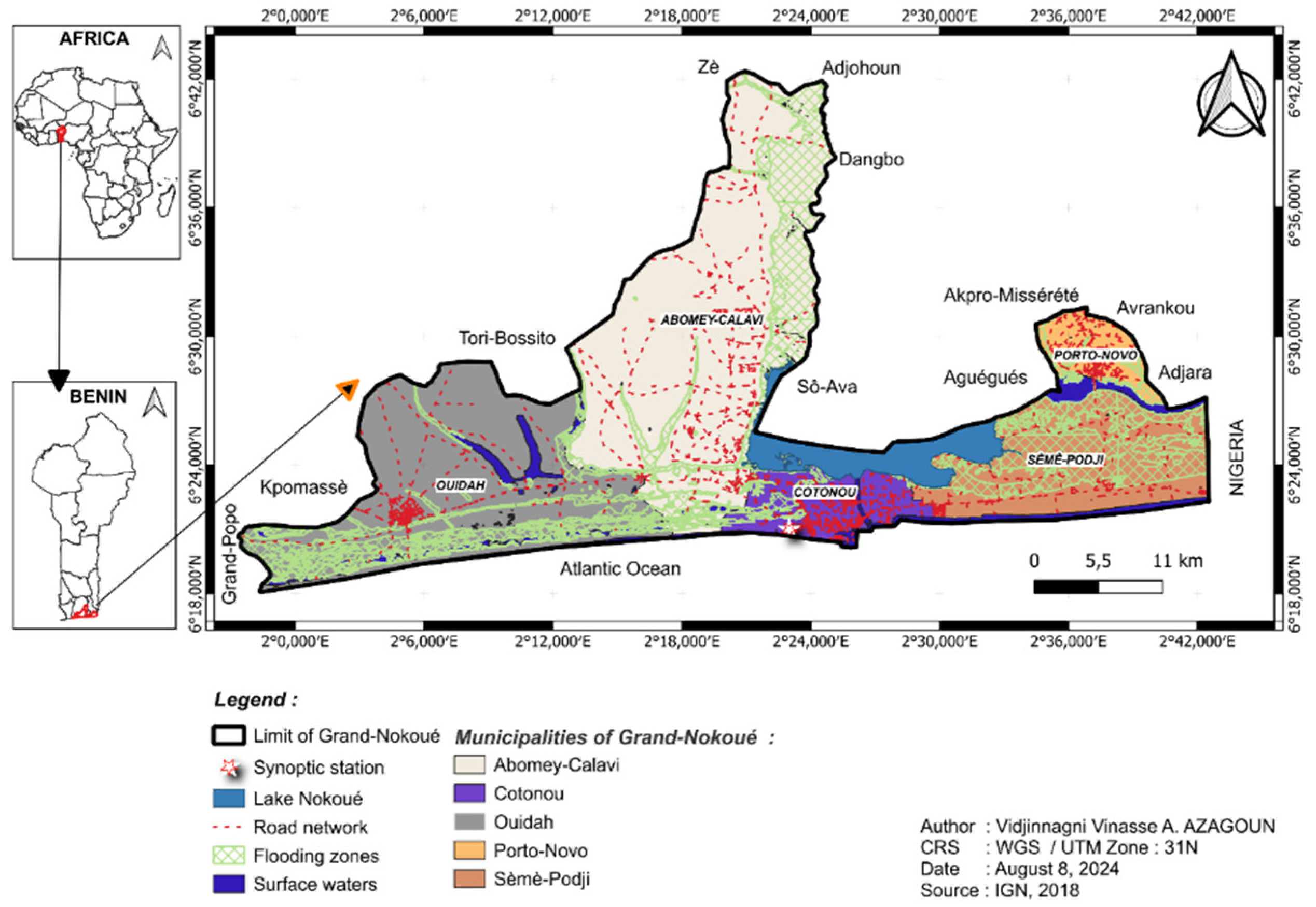
Located between 6°18′ and 6°30′ north latitude and 2°02′ and 2°40′ east longitude, Great Nokoué bordered north by inland municipalities, south by the Atlantic Ocean, east by Nigeria, and west by the municipality of Great-Popo (
Figure 1). This area covers 380 km² in southern China and comprises the municipalities of Abomey-Calavi, Cotonou, Ouidah, Porto-Novo and Semè-Podji. These towns have developed around a well-stocked hydrological network, including Lake Nokoué (the largest lake in Benin, covering 150 km²), Porto-Novo Lagoon (35 km²), Ouidah Lagoon (40 km²), and Lake Toho (15 km²). The territory of Great Nokoué is largely occupied by hydromorphic, ferralitic and ferruginous tropical soils [
19]. Great Nokoué has a synoptic station (6° 21‘ N and 2° 23′E) that records and supplies the various climatic parameters of the region.
The population of Great Nokoué rose from 604,106 in 1979 to 1,388,190 in 2002, reaching 1,984,206 in 2013. This region will be home to 3,141,482 inhabitants by 2025, or 25% of Benin’s population [
22]. This population growth justifies the presence of goods and services that are likely to be impacted by extreme climatic events, hence the need to understand the hydroclimatic dynamics of the territory.
2.2. Data Collection
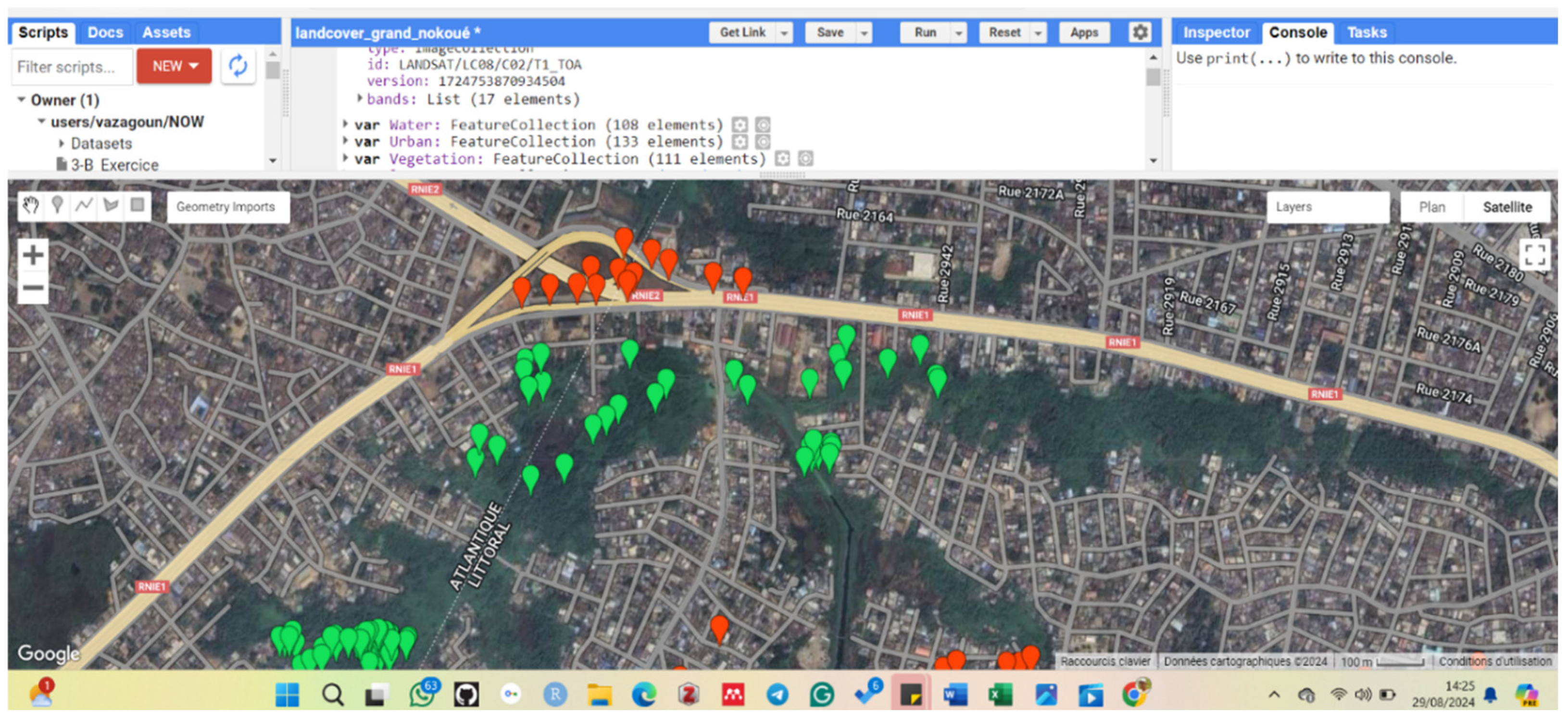
The data used in this study were related mainly to climate and land use. The climatic data are related to precipitation and temperature (minimum and maximum), two main variables that are crucial for assessing climatic risk. These daily time-step data for the period 1991 to 2020 come from the Cotonou synoptic station (6° 21′ N and 2° 23′E) and are supplied by the Benin National Meteorological Agency (Météo-Bénin). The land cover data are derived from level 1 satellite images from the second Landsat 8 collection, which are available from the USGS Earth Explorer website. These are top-of-atmosphere (TOA) reflectance images from the Landsat 8 OLI/TIRS sensor. These images were downloaded from the Google Earth Engine for the years 2014, 2018 and 2020. Using the Google Earth Engine (GEE), we first selected the most cloud-free images from bands 2, 3, and 4 for each annual period. This was followed by supervised classification on the basis of knowledge of the study environment. This classification considers four main environmental factors of the urban environment: vegetation, water bodies, bare soil and built-up areas.
Figure 2 shows a manipulation capture of the Google Earth Engine (GEE) interface for supervised classification.
2.2. Data Processing and Analysis
The climate data were first subjected to quality control using Rclimdex, a climate algorithm for use with the R environment. This tool is recommended by the Expert Team on Climate Change Detection Monitoring and Indices (ETCCDMI) for its ability to identify errors in daily data collection, detect indicators of climate change and facilitate the monitoring of extreme weather events [
23]. Analysis of the variation in monthly climatic parameters (precipitation, temperature) was carried out via box plots. These graphs made it possible to represent the statistical distribution of the data in a way that was clear and accessible to a wide range of users. In addition to showing the median and quartiles, these box plots make it easier to observe symmetry or asymmetry in the distribution of climate data [
24] and to identify extreme values and anomalies by highlighting highly concentrated or dispersed data.
Land cover data from the Google Earth Engine (GEE) were imported into QGIS software version 3.36.3 to calculate class areas and map their dynamics. The area values calculated through correlograms with R software version 4.4.0 [
25] were used to determine the relationships between hydroclimatic extremes and the dynamics of land cover elements. The same software is used for the main statistical tests. These tests are described below:
2.3.1. Mann‒Kendall Test
The Mann‒Kendall test was used to analyze temporal trends in climatic parameters. It is a nonparametric statistical test, as it does not assume the underlying distribution of the data. It is often used for trend analysis of climatological and hydrological time series data [
24,
26]. It is used to examine the existence of a linear trend (upward or downward) in a time series. The H
0 hypothesis tested at the 5% threshold is the nonexistence of a trend. If the p-value is lower than the significance threshold chosen for this study (5%), the H
0 hypothesis is rejected, and we conclude that a significant trend exists. This test was performed with the trend package of R software [
25,
27]. The Mann‒Kendall statistical formula can be described via Eq. (1) and Eq. (2):
(1)
where n is the sample length and where xi and xj are i = 1, 2... n 1 and j = i+1... n.
with
(2)
Si le nombre d’enregistrements utilisés pour le test est supérieur à 10 (N > 10), la statistique de distribution moyenne est approximativement égale à zéro et la variance de « S » est calculée à l’aide des équations Eq. (3) et Eq. (4).
(3)
(4)
Zc is used to assess whether there is a statistically significant trend. A positive Zc value indicates an upward trend, whereas a negative Zc value indicates a downward trend for the period. As the test is two-tailed, i.e., |Zc| > z/2, the null hypothesis is rejected. Positive Zc values indicate an upward trend and negative values indicate a downward trend for the parameter in question.
2.3.2. Estimating Sen’s Slope
After positive or negative increases were determined via the Mann–Kendall test, Sen’s slope estimation test was used to determine whether the magnitude of these trends decreased or increased. Often applied to long series, the Sen slope test is used to assess the increase and decrease in the magnitude of the slope corresponding to Mann‒Kendall values [
27,
28]. Slope pairs can be calculated for all data showing a linear trend via a simple, systematic nonparametric procedure whose equation is Eq. (5):
(5)
where Ti is the slope and xj and xk are the data values at times j and k, respectively. The average of the n values of Ti is coded as Sen’s slope estimator (Qi) and is calculated via Eq. (6).
(6)
2.3.3. Extreme Value Theory
In this study, extreme value theory is used to analyze trends in rare climatic events. Unlike the descriptive indices developed by the Expert Teamon Climate Change Detection and Indices (ETCCDI), which focus on moderate extreme events occurring several times a year. Extreme value theory has the advantage of identifying rare extreme events associated with high return periods, such as 2, 5, 10, 50 and 100 years [
29,
30,
31]. Using this theory, we were able to carry out a holistic trend analysis of monthly extreme events representing the 99th percentiles of three-day accumulations of climatic parameters (rainfall, minimum and maximum temperatures). The value of using climate parameter accumulations lies in their ability to improve climate models by providing integrated data over longer periods, enabling better preparation for extreme weather events. To analyze the frequency of extremes, we used Gringorten’s plot formula, whose equation is Eq. (7):
(7)
With
qi = probability of exceedance; N = number of observations in the database; i = rank of the specific observation; i = 1 is the largest, and i = N is the smallest. a = Estimation constant = 0.44
2.3.4. Qualitative test of the Gumbel fit
To determine the extremes associated with specific return intervals, the data were fitted to the Gumbel extreme value distribution, whose equation is Eq. (8):
(8)
where x represents the observed data and where u and x are parameters that shape the distribution.
where is the mean of the observations and S_x is the square root of the variance, also known as the standard deviation.
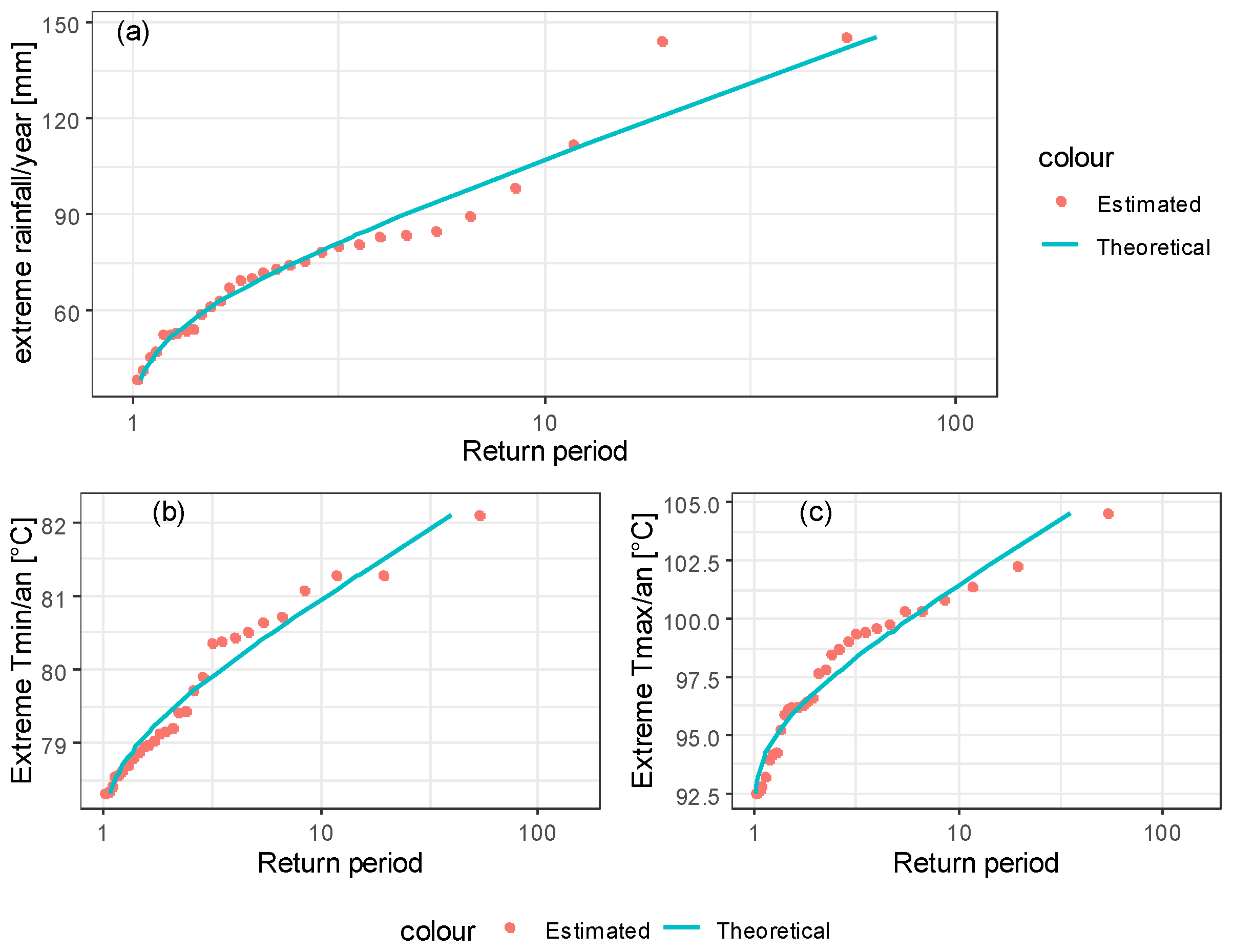
Gumbel’s law offers a better fit for maximum values. The points align better with the trend line.
Figure 3 below shows the correlation between the observed (estimated) and fitted (theoretical) values and Gumbel’s law for each of the climatic parameters. The maximum values fit very well with Gumbel’s law.
3. Results
3.1. Analysis of Seasonal and Interannual Variability
3.1.1. Seasonal Variability in Climatic Parameters
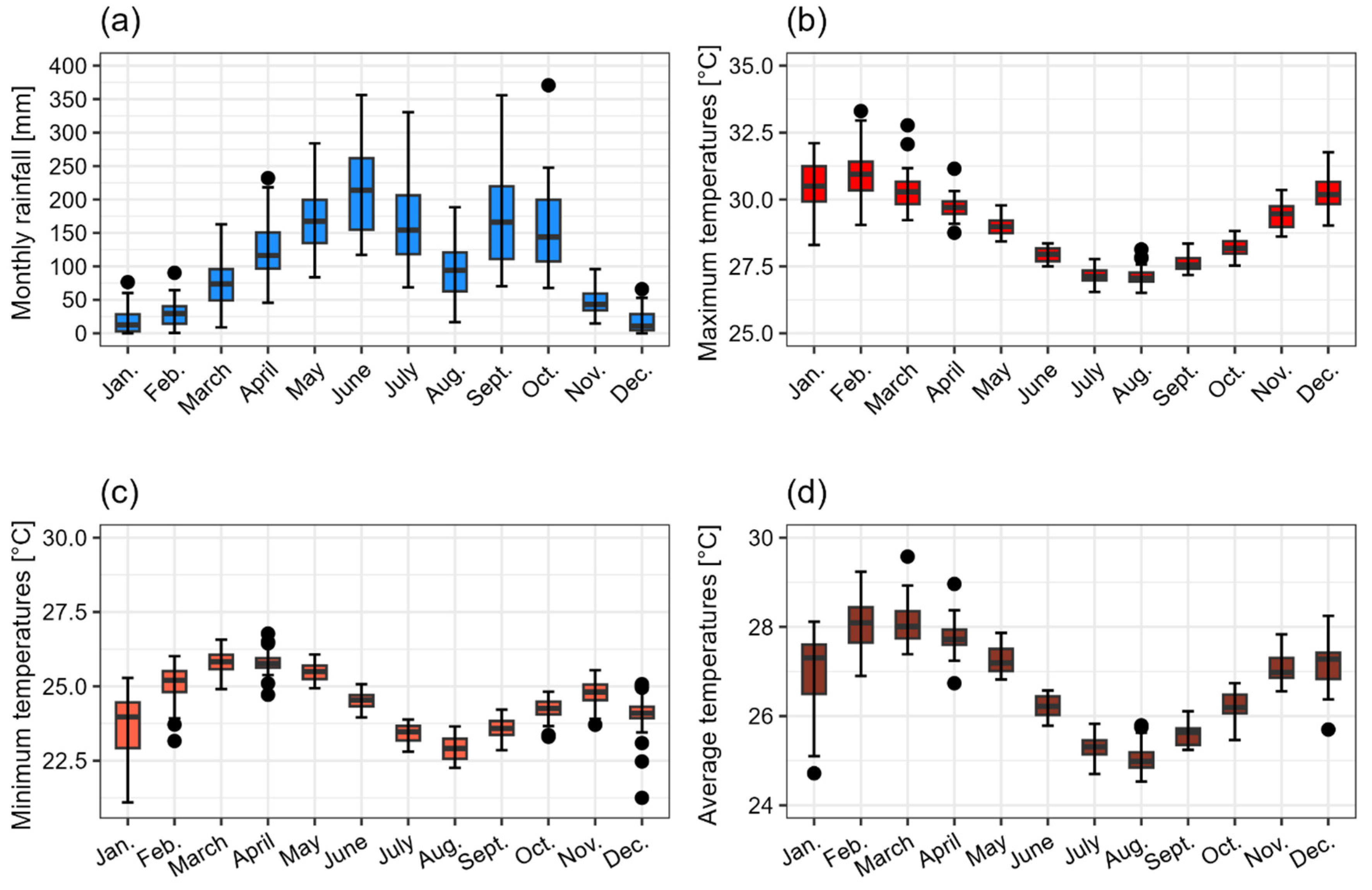
Figure 4 below shows whisker boxes illustrating the seasonal evolution of climatic parameters over the period 1991 to 2020 at the Cotonou synoptic station.
Figure 4a shows that the rainfall pattern in this part of Benin is bimodal, with high variability in monthly averages (from 18.4 to 212.80 mm). April to July and September to October are the wettest months, with the first peak occurring in June (212.80 mm) and the second occurring in September (174.62 mm).
Figure 4b shows that the average maximum (daytime) temperatures range from 27.15 to 30.98°C. November to March are the warmest months, with a higher peak (30.98°C) in February. On the other hand, July and August had the lowest daytime temperatures, with values of 27.16 and 27.15°C, respectively.
Figure 4c shows the seasonal trend in average minimum (nighttime) temperatures. The analysis of this figure reveals that nighttime temperatures fluctuate throughout the year, with peaks occurring from March to April (average values of 25.83°C and 25.82°C, respectively), and January and December are the coolest months, with average values of 23.56°C and 24.05°C, respectively. Three years of lower extremes were recorded in December alone (21.25°C, 22.47°C, and 23.09°C in 2015, 1994 and 2011, respectively).
The average monthly temperatures follow a similar pattern to the maximum monthly temperatures, with higher peaks in February and March and lower peaks in July and August. Averages range from 25.03 to 28.10°C and are observed in August and March, respectively (
Figure 4d).
3.1.2. Analysis of Temporal Trends in Climatic Parameters
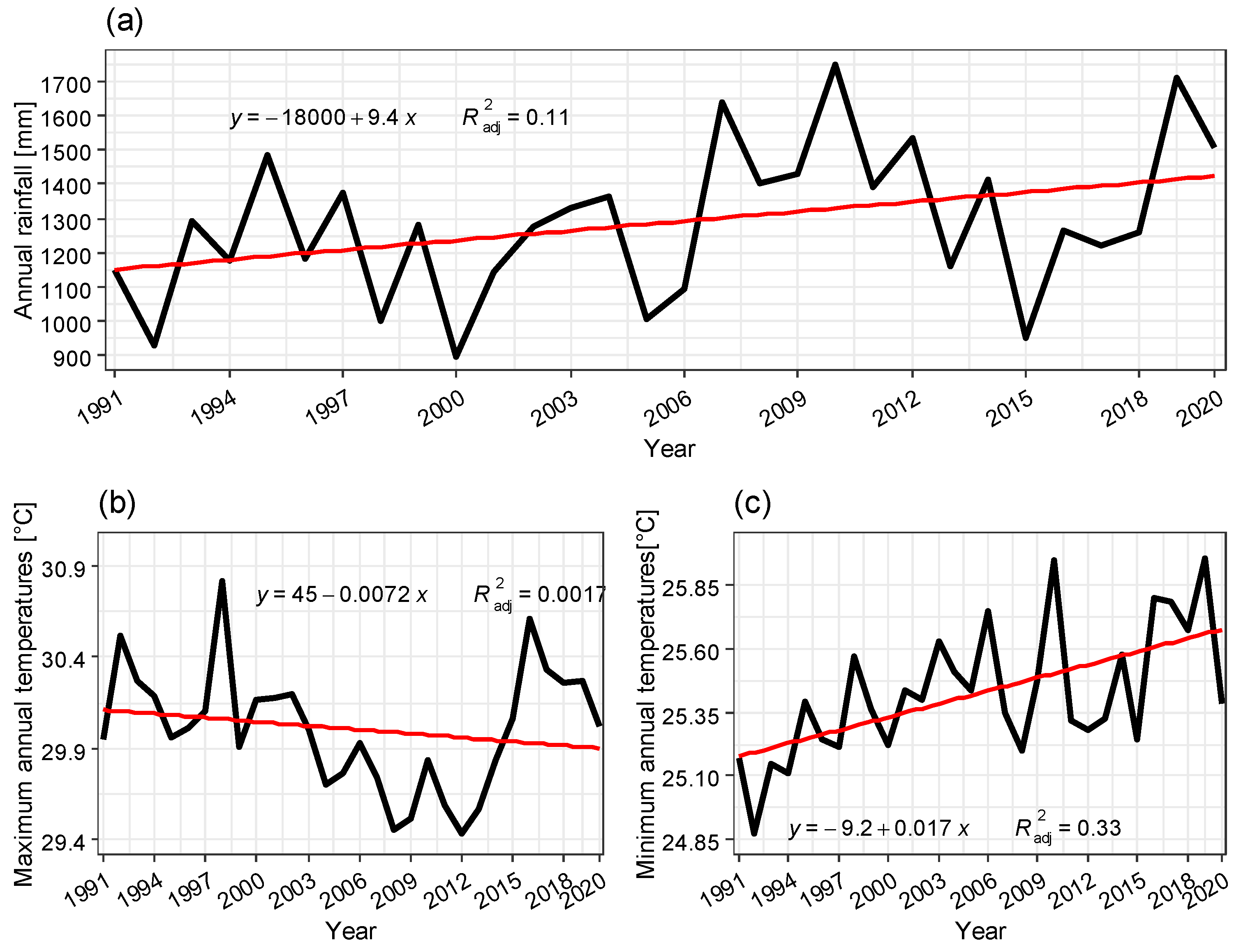
The interannual evolution of minimum and maximum precipitation and temperature from 1991 to 2020 is shown in
Figure 5. The analysis of this figure reveals a variation in all the climatic parameters of interest.
From the statistical results of the trend and slope level tests recorded in
Table 1, we observe positive tau values of 0.25 and 0.14, respectively, for precipitation and minimum temperatures for the Mann–Kendall trend test, with p values below the 5% threshold (0.04 and 0.001). These values imply that the increasing trends observed in precipitation and minimum temperatures are significant. On the other hand, the decrease in the maximum temperature is not significant (tau= -0.14, p-value=0.30). The median values of Sen’s estimation test reveal that 50% of the slopes are greater than or equal to 11.22, i.e., an annual increase of 11.22 mm of rainfall. In terms of temperature, there was an annual increase of 0.02°C at night and an annual decrease of 0.01°C during the day from 1991 to 2020.
3.2. Seasonal Frequency Analysis of the Extrêmes
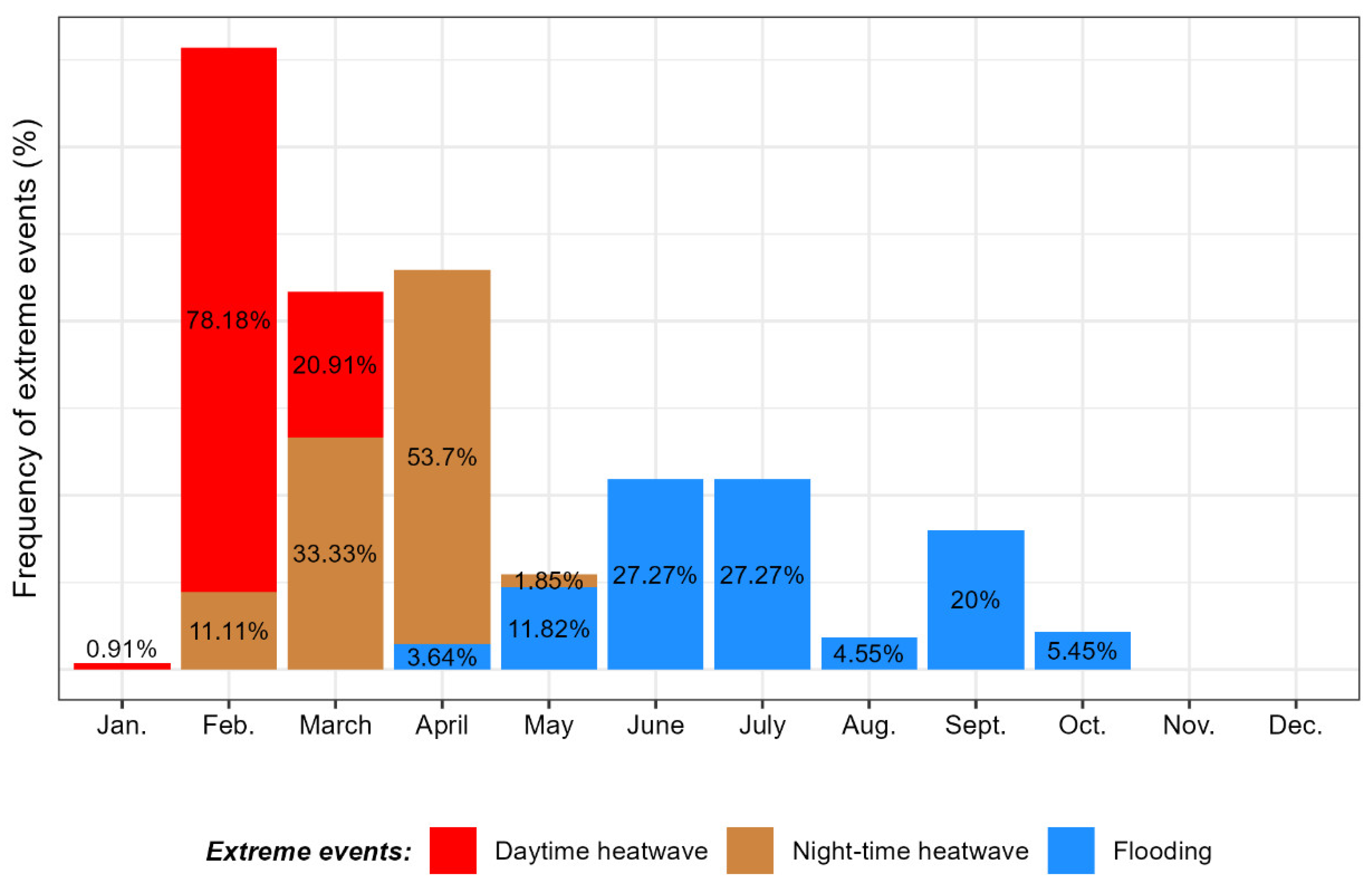
The monthly frequency of occurrence of extreme events over the 30 years (1991 to 2020) is illustrated in Figure.6 below. This figure shows that precipitation extremes occur over seven consecutive months, starting in April, whereas daytime temperature extremes occur over three months, from January to February, and nighttime temperature extremes occur over four months, from February to May. These results show that flooding is the most recurrent climatic hazard.
Figure 6.
Seasonal frequency of extreme hydroclimatic events in Great Nokoué.
Figure 6.
Seasonal frequency of extreme hydroclimatic events in Great Nokoué.
The proportions of extreme rainfall events in June (27.27%), July (27.27%) and September (20%) are greater than 15.71%, which is expected (
Table 2). The chi-square test revealed that the probability of occurrence of extreme rainfall events was below the threshold set at 5% (
p-value < 0.001). This low p-value implies that the monthly disproportion in flood occurrence frequencies observed in Great Nokoué is statistically significant. Furthermore, the proportion of extreme daytime temperature events observed (78.18%) in February was higher than expected (36.6%). Similarly, in April, a higher percentage (53.7%) than expected (36%) was recorded. As the p values are all less than 0.05, the initial hypothesis H
0 cannot be accepted, and we can conclude that the months with high proportions of extreme events are not linked to chance.
3.3. Return Period Analysis of Extreme Events
Table 3 below shows the return periods (2, 5, 10, 20, 50 and 100 years) and the results of the statistical tests used to assess the uncertainty associated with the estimates. An analysis of this table reveals that the return period of percentiles (99th) of three-day rainfall totals varies over periods of 2, 5, 10, 20, 50 and 100 years. Extreme rainfall with a one-in-two probability of occurring in Greater Nokoué had a value of 69.33 mm. These values remained constant for all events. The same is true for the percentiles of three-day cumulative daytime temperatures, which rose from 96.88°C in 2 years to 107.07°C in 100 years, and nighttime temperatures, which rose from 79.42°C to 82.85°C for return period frequencies. The coefficients of determination for each parameter are 0.97, 0.98 and 0.95, respectively. These values are very close to 1, with
p-values all less than 0.05. High values of the coefficient of determination indicate that extreme events are likely to occur.
3.4. Land Cover Dynamics
The land use dynamics from 2014 to 2020 are represented by the maps in
Figure 7. Observations of these maps reveal that the surface area of built-up areas dominates that of the other land use elements highlighted (water/wetlands, vegetation and night soils). This surface area increases from one year to the next. It rose from 496.93 km
2 in 2014 to 454.65 km
2 in 2018 and will reach 561.79 km
2 in 2020. This evolution has resulted in a decrease in the natural elements of the environment [
32,
33].
3.5. Relationships between Hydroclimatic Extremes and Urban Environmental Factors
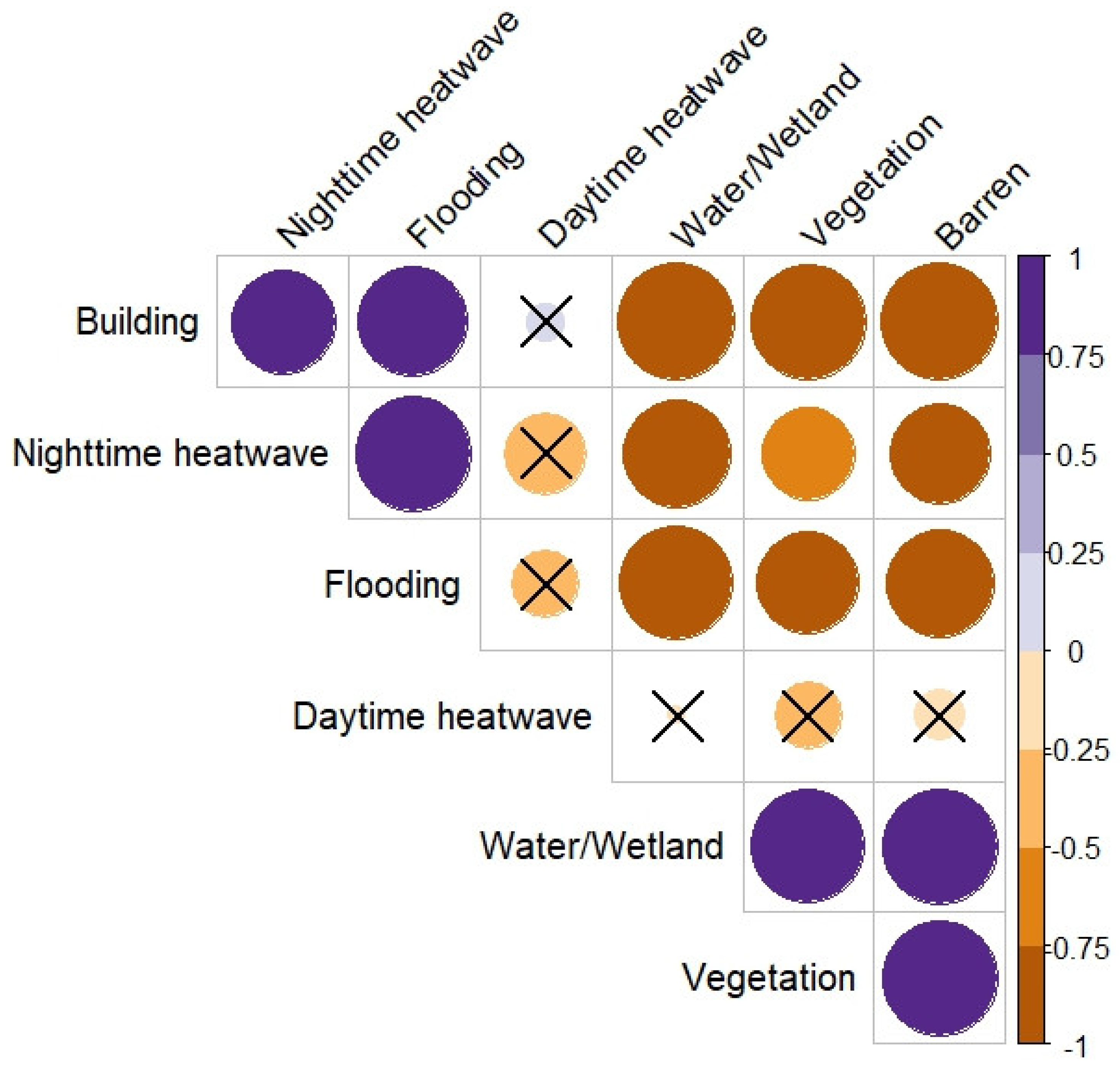
A correlation matrix based on Person’s correlation formula was used to identify probable relationships between the frequency of occurrence of hydroclimatic extremes and environmental factors in the urban environment. This matrix was represented by the correlogram combined with the significance test of the relationship at the 0.05 threshold. Nonsignificant correlations, with
p-value > 0.05 [
27], are crossed out (
Figure 8). This correlogram indicates that buildings are positively correlated with the three types of extreme weather events highlighted. This implies that the development of buildings has increased the frequency of climatic events in Great Nokoué. The phenomenon is most pronounced with flooding and nighttime heat events, for which the relationships are highly significant (
p-value < 0.001). However, these events are negatively correlated with water bodies (r = -0.93 and -0.85 with
p-value < 0.001), vegetation (r= -0.77 and -0.64 with
p-value < 0.001) and bare soil (r = -0.85 and -0.77 with
p-value < 0.001), indicating that a reduction in the surface area of the latter increases the frequency of flooding and nighttime heat events.
4. Discussion
4.1. Variability in Parameters and Occurrence of Extreme Climatic Events
The main climatic parameters (precipitation and maximum and minimum temperatures) identified in the Great Nokoué region all show both intraseasonal and interannual variability. The seasonal variability in these parameters is thought to be the cause of the poor distribution of rainfall, which could lead to both an increase in the frequency of climatic extremes and a disruption of the start-of-season dates and water cycles. These results corroborate the research Oyede et al. [
17], who revealed that the total number of rainy days and temperature trends in Benin show strong inter- and intra-annual variability. Similarly, Kingbo et al. [
34] reported that the climate in the southern part of Benin was influenced by the fluctuating rainfall patterns observed in West Africa in late 1960s and early 1970s. This climate variability has an impact on daily urban life and prompts behavioral adaptation strategies for perceived and expected impacts, even over short periods [
35].
Furthermore, significant disproportions (
p-values < 0.001) were observed in the frequency of occurrence of extremes. The high proportions of extreme frequencies observed are therefore not linked to chance but rather to the variability and intensity of the parameter under consideration. In fact, the months with the highest occurrence of extremes (
Figure 6) correspond to the months with the greatest variability over the thirty-year study period (
Figure 4). The research results of several authors, such as Asseng et al.[
3], Meehl and Tebald [
4], Chaigneau et al.[
14], point in the same direction, showing that the recurrence of extreme weather events such as floods, heat waves, droughts and storms is linked to climate variability and change. However, Mann‒Kendall statistical tests revealed significant upward trends for precipitation (tau = 0.25 and
p-value = 0.04) and nighttime temperatures (tau = 0.41 and
p-value = 0.001), which could explain the increased frequency and magnitude of extreme weather events, calling into question the population’s ability to adapt to these events [
9]. These rising trends could be linked to the presence of water bodies and the microclimate generated by activities in urban environments. Indeed, rising temperatures due to the effects of urban heat islands increase temperatures[
36], which could modify the water cycle. Tabari [
10] reported that rainfall frequency and intensity depend on the hydrological cycle. Although the daytime temperatures show a downward trend (
Figure 5b), their theoretical extremes, as well as those estimated from the Gumbel goodness-of-fit test, are steadily increasing, as are the precipitation and nighttime temperatures over return periods of 2, 5, 10, 50 and 100 years, which would justify the insignificance of their trend (
Table 3). The values of the coefficients of determination show (
Table 3) that flood, nocturnal and diurnal heatwave events are therefore likely to recur at return periods of 2, 5, 10, 50 and 100 years, with consequences for urban development factors. These findings corroborate those of Egerer et al.[
35], who indicate that urban populations face longer and more frequent periods of extreme heat, drought and flooding. Benin’s National Adaptation Plan (PNA) on climate change shows that changes in climatic parameters have impacts on eight of the country’s priority development sectors[
16].
4.2. Urban Dynamics and Frequency of Hydroclimatic Extremes
The aim of this study is to highlight the relationships between urban land use elements (buildings, water/wetlands, bare soil and vegetation) and the frequency of occurrence of climatic phenomena that directly influence water resources and can have significant environmental, social and economic consequences. The development of built-up areas is clearly the main factor influencing the frequency of rainwater flooding and heat waves, both at night and during the day (Figure 9). Indeed, the construction of buildings and infrastructure reduces the amount of green spaces and water bodies/wetlands that are supposed to regulate the atmospheric temperature [
37]. Reducing the latter would lead to a warmer atmosphere [
38] capable of retaining more moisture, which could lead to more intense rainfall. For Tabari [
10] and Hong et al. [
39], rising temperatures intensify the hydrological cycle, which is likely to increase the intensity of extreme precipitation and the risk of flooding. Urban sprawl, as seen in Great Nokoué, puts the region at risk of more intense heat waves (
Table 3). Dossou et al. [
40], Egerer [
35], and Stoneet al. [
41] reported that variations in urban impermeable land cover strongly influence the frequency and severity of heat events. Indeed, Ecological infrastructures help regulate local temperatures and mitigate the effects of urban heat islands.[
42]. World Bank Group [
13] for example, recommends reducing deforestation to mitigate climate risk.
Conclusion
Extreme climatic events in urban areas are becoming increasingly frequent and constitute a major development problem. This study analyzed the frequency of occurrence of hydroclimatic events and highlighted their relationship with land-use dynamics in Grand Nokoué. Pluvial flooding and diurnal and nocturnal heat waves were found to be the main urban hydroclimatic events, with intensities dependent on variations in impervious ground cover. In fact, it has been observed that increases in diurnal and nocturnal heat influence the frequency and intensity of rainfall leading to flooding. As a result, flooding is the most recurrent climatic hazard, occurring on average seven months of the year. As urbanization accelerates, the frequency and severity of climatic hazards in cities will increase. To ensure sustainable development, the following measures need to be taken into account in urban planning:
- the interaction between vegetation, water bodies/wetlands, bare soil and buildings ;
- the integration of green spaces,
- promoting urban agriculture and improving drainage infrastructure.
Author Contributions
Conceptualization, V.V.A.A.; methodology, V.V.A.A. and K.K.; software, V.V.A.A.; validation, K.S.K.; formal analysis, V.V.A.A. and K.K.; investigation, V.V.A.A.; resources, V.V.A.A. and K.S.K.; writing—original draft preparation, V.V.A.A.; writing—review and editing, V.V.A.A.; visualization, V.V.A.A. and K.K.; supervision, K.S.K. and E.W.V.; project administration, K.S.K.; funding acquisition, V.V.A.A. All authors have read and agreed to the published version of the manuscript.
Funding
This research was funded by the Regional Center of Excellence on Sustainable Cities in Africa (CERViDA-DOUNEDON), the Association of African Universities (AUA), and the World Bank. This research is funded under number IDA 5360 TG.
Institutional Review Board Statement
Not applicable.
Informed Consent Statement
Not applicable.
Data Availability Statement
Data will be made available upon request.
Acknowledgments
The authors would like to thank the Regional Centre of Excellence on Sustainable Cities in Africa (CERViDA-DOUNEDON), the Association of African Universities and the World Bank Group for the financial support that made this study possible. Thanks are also due to the African Cities Lab for its training in urban data management. possible. Thanks are also due to the African Cities Lab for its training in urban data management.
Conflicts of Interest
The authors declare that they have no conflicts of interest.
References
- Nehlig, P.; What do the geological archives tell us about CO2 and climate? p. 7, Jan. 2006. Available online: https://www.researchgate.net/publication/274717251 (accessed on 8 December 2023).
- Malhi, Y.; Franklin, J.; Seddon, N.; Solan, M.; Turner, M.G.; Field, C.B.; Knowlton, N. Climate change and ecosystems: threats, opportunities and solutions. Phil. Trans. R. Soc. B, vol. 375, no. 1794, p. 20190104, Mar. 2020. https://doi.org/10.1098/rstb.2019.0104. [3] Asseng, S.; Ewert, F.; Rosenzweig, C.; Jones, J.W.; Hatfield, J.L.; Ruane, A.C.; Boote, K.J.; Thorburn, P.J.; Rötter, R.P.;Cammarano, D.; Brisson, N.; Basso, B., Martre, P.; Aggarwal, P.K.; Angulo, C.; Bertuzzi, P.; Biernath, C.; Challinor, A.J.;Doltra, J.; Gayler, S.; Goldberg, R.; Grant, R.; Heng, L.; Hooker, J.; Hunt, L.A.; Ingwersen, J.; Izaurralde, R.C.; Kersebaum, K.C.; Müller, C.; Naresh Kumar, S.; Nendel, C.; O’Leary, G.; Olesen, J.E.; Osborne, T.M.; Palosuo, T.; Priesack, E.; Ripoche, D.; Semenov, M.A.; Shcherbak, I.; Steduto, P.; Stöckle, C.; Stratonovitch, P.; Streck, T.; Supit, I.; Tao, F.; Travasso, M.; Waha, K.; Wallach, D.; White, J.W.; Williams, J.R.; Wolf, J. Uncertainty in simulating wheat yields under climate change. Nature Clim Change, vol. 3, no. 9, pp. 827–832, Sep. 2013. [CrossRef]
- Meehl, G.A.; Tebaldi, C. More Intense, More Frequent, and Longer Lasting Heat Waves in the 21st Century. Science, vol. 305, no. 5686, pp. 994–997, Aug. 2004. [CrossRef]
- C40Cities, ‘Integrating adaptation to climate change: A guide for planners and adaptation professionals’. Global Platform for Sustainable Cities, 2021. Accessed: Sep. 04, 2024. [Online]. Available: www.c40knowledgehub. (accessed on 4 September 2024).
- Lin, L.; Gao, T.; Luo, M.; Ge, E.; Yang, Y.; Liu, Z.; Zhao, Y.; Ning, G. , ‘Contribution of urbanization to the changes in extreme climate events in urban agglomerations across China. Science of The Total Environment, vol. 744, p. 140264, Nov. 2020. [CrossRef]
- Lin, B.B.; Egerer, M.H.; Liere, H.; Jha, S.; Bichier, P.; Philpott, S.M. Local- and landscape-scale land cover affects microclimate and water use in urban gardens. Science of The Total Environment, 2018; 610–611, 570–575. [Google Scholar] [CrossRef]
- Patz, J.A.; Campbell-Lendrum, D.; Holloway, T.; Foley, J.A. Impact of regional climate change on human health. Nature, 2005; 438, 310–317. [Google Scholar] [CrossRef]
- Calvin, K. Dasgupta; D., Krinner, G.; Mukherji, A.; Thorne, P.W.; Trisos, C.; Romero, J.; Aldunce, P.; Barrett, K.; Blanco, G.; et al. IPCC, 2023: Climate Change 2023: Synthesis Report. Contribution of Working Groups I, II and III to the Sixth Assessment Report of the Intergovernmental Panel on Climate Change [Core Writing Team, H. Lee and J. Romero (eds.)]. IPCC, Geneva, Switzerland.. Intergovernmental Panel on Climate Change (IPCC), Jul. 2023. [CrossRef]
- Tabari, H. Climate change impact on flood and extreme precipitation increases with water availability. Sci Rep, vol. 10, no. 1, p. 13768, Aug. 2020. [CrossRef]
- Egerer, M.H.; Lin, B.B.; Kendal, D. Temperature Variability Differs in Urban Agroecosystems across Two Metropolitan Regions. Climate, 2019; 7, 50. [Google Scholar] [CrossRef]
- UN-Habitat, Ed., Envisaging the future of cities. in World cities report, no. 2022. Nairobi, Kenya: UN-Habitat, 2022.
- World Bank Group, ‘Bénin – National report on climate and development. CCDR Series. © Washington, DC: World Bank. http://hdl.handle.net/10986/40688 License: CC BY-NC-ND 3.0 IGO.. Washington, 2023. Accessed: Dec. 08, 2023. [Online]. Available online: https://openknowledge.worldbank.org/handle/10986/40688.
- Chaigneau, A.; STIEGLITZ, T.; Okpeitcha, V. Assogba,A.; Sohou, Z.; Peugeot, P.; MOREL, Y. Impact of global change on lagoon systems in West Africa: the case of Lake Nokoué in Benin. Jul. 2020. Accessed: Nov. 23, 2023. [Online]. Available online: https://horizon.documentation.ird.fr/exl-doc/pleins_textes/2021-08/010082429.pdf.
- Djohy, G.L.; Edja, A.H. Effect of climatic variability on water resources and adaptation strategies of livestock farmers and market gardeners in North Benin. p. pp.83-91, Summer 2018. Accessed: Jan. 19, 2024. [Online]. Available online: https://hal.science/hal-02046892/document.
- Ministry for the Environment and Sustainable Development (MCVDD), ‘Benin’s National Climate Change Adaptation Plan’. May 2022. Accessed: Sep. 30, 2024. [Online]. Available online: https://unfccc.int/sites/default/files/resource/PNA_BENIN_2022_0.pdf.
- Oyede, M.I.; Hounzime, S.; Agbokou, I.; Alhassane, A.; Yabi, I. Spatio - temporal characteristics of climate variability in Benin (West Africa). ESJ, 2022; 18, 240. [Google Scholar] [CrossRef]
- Houessinon, D.R.B.; Ognondoun, A.; Tchibozo, E.A.M.; YabI, I. Adaptation and flood risk reduction strategies in the Grand Nokoué agglomeration (southern Benin)’.Accessed: Nov. 11, 2023. [Online]. Available online: https://revues.imist.ma/index.php/EGSM/article/view/39697.
- Blalogoé, C.P. Stratégies de lutte contre les inondations dans le grand Cotonou: diagnostic et al.ternative pour une gestion durable. Unique doctoral thesis, Abomey-Calavi, Université d’Abomey-Calavi, Bénin, 2014.
- Atchadé, A.A.G. Impacts of climate dynamics and land use on water resources in the zou river watershed in southern Benin. PhD thesis, University of Abomey-calavi/EDP/FLASH, Benin, 2014.
- Amontcha, A.A.M.; Djego, J.G.; Lougbegnon, T.O. and Sinsin, B.A., ‘Typology and distribution of public green spaces in Grand Nokoué (southern Benin). ESJ, 2017; 13, 79. [Google Scholar] [CrossRef]
- National Institute of Statistics and Economic Analysis (INSAE). Provisional results of the RGPH 4. MDAEP - Ministry of Développement, de l’Analyse Economique et de la Prospective, Cotonou, Benin, 2013.
- Zhang, X.; Alexander, L.; Hegerl, G.C.; Jones, P.; Tank, A.K.; Peterson, T.C.; Trewin, B.; Zwiers, F.W. Indices for monitoring changes in extremes based on daily temperature and precipitation data. WIREs Climate Change, 2011; 2, 851–870. [Google Scholar] [CrossRef]
- Panda, A. and Sahu,N. Trend analysis of seasonal rainfall and temperature pattern in Kalahandi, Bolangir and Koraput districts of Odisha, India. Atmospheric Science Letters, 2019; 20, e932. [Google Scholar] [CrossRef]
- R Core Team, R. R. A Language and Environment for Statistical Computing. (2023). R Foundation for Statistical Computing, Vienna, Austria. Accessed: Jan. 23, 2024. [Online]. Available online: https://www.R-project.org/.
- Güçlü, Y.S. Improved visualization for trend analysis by comparing with classical Mann-Kendall test and ITA. Journal of Hydrology, 2020; 584, 124674. [Google Scholar] [CrossRef]
- Pohlert, T. trend: Non-Parametric Trend Tests and Change-Point Detection. (2023). Accessed: Aug. 23, 2024. [Online]. Available online: https://CRAN.R-project.org/package=trend.
- Guo, A.; Zhang, Y.; Zhong, F.; Jiang, D. Spatiotemporal Patterns of Ecosystem Service Value Changes and Their Coordination with Economic Development: A Case Study of the Yellow River Basin, China. IJERPH, 8474; 17, 8474. [Google Scholar] [CrossRef]
- Houngue, N.R.; Almoradie, A.D.S.; Thiam, S.; Komi, K.; Adounkpè, J.G.; Begedou, K.
- Evers, M. Climate and Land-Use Change Impacts on Flood Hazards in the Mono River Catchment of Benin and Togo. Sustainability, vol. 15, no. 7, p. 5862, Mar. 2023. [CrossRef]
- Klassou, K.S.; Komi, K. Analysis of extreme rainfall in Oti River Basin (West Africa). Journal of Water and Climate Change, 1997; 12, 1997–2009. [Google Scholar] [CrossRef]
- Ogega,O. M.; Scoccimarro, E.; Misiani, H.; Mbugua, J. Extreme climatic events to intensify over the Lake Victoria Basin under global warming. Sci Rep, 9729; 13, 9729. [CrossRef]
- Ren, Q.; He, C.; Huang, Q.; Zhang, D.; Shi, P.; Lu, W. Impacts of global urban expansion on natural habitats undermine the 2050 vision for biodiversity. Resources, Conservation and Recycling, 2023; 190, 106834. [Google Scholar] [CrossRef]
- Seifollahi-Aghmiuni, S.; Kalantari, Z.; Egidi, G.; Gaburova, L.; Salvati, L. Urbanisation-driven land degradation and socioeconomic challenges in peri-urban areas: Insights from Southern Europe. Ambio, 2022; 51, 1446–1458. [Google Scholar] [CrossRef]
- Kingbo, A.; Teka, O.; Aoudji, A.K.N.; Ahohuendo, B. and Ganglo, J.C. Climate Change in Southeast Benin and Its Influences on the Spatio-Temporal Dynamic of Forests, Benin, West Africa. Forests, 2022; 13, 698. [Google Scholar] [CrossRef]
- Egerer, M.; Lin, B.; Kendal, D. Temperature Variability Differs in Urban Agroecosystems across Two Metropolitan Regions. Climate, 2019; 7, 50. [Google Scholar] [CrossRef]
- Krsnik, G. Is Zagreb Green Enough? Influence of Urban Green Spaces on Mitigation of Urban Heat Island: A Satellite-Based Study. Earth, 2024; 5, 604–622. [Google Scholar] [CrossRef]
- Coronel, S.; . Feldman, A.R.; Jozami, S.; Facundo, E.; Piacentini, K.D.; Dubbeling, M.J.; Escobedo, F. Effects of urban green areas on air temperature in a medium-sized Argentinian city. AIMS Environmental Science, 2015; 2, 803–803. [Google Scholar] [CrossRef]
- Intergovernmental Panel On Climate Change (Ipcc), Climate Change 2022 – Impacts, Adaptation and Vulnerability: Working Group II Contribution to the Sixth Assessment Report of the Intergovernmental Panel on Climate Change, 1st ed. Cambridge University Press, 2023. [CrossRef]
- Hong, S.-H.; Jin, H.-G.; Baik, J.-J. Detection of urban effects on precipitation in the Seoul metropolitan area, South Korea. Urban Climate, 2024; 53, 101773. [Google Scholar] [CrossRef]
- Dossou, J.F.; Li, X.X.; Kang, H. ; Boré,A. Impact of climate change on the Oueme basin in Benin. Global Ecology and Conservation, 2021; 28, e01692. [Google Scholar] [CrossRef]
- Stone, B.; Hess, J.J.; Frumkin, H. Urban Form and Extreme Heat Events: Are Sprawling Cities More Vulnerable to Climate Change Than Compact Cities? Environ Health Perspect, 2010; 118, 1425–1428. [Google Scholar] [CrossRef]
- Dawson, N.; Martin, A. Assessing the contribution of ecosystem services to human wellbeing: A disaggregated study in western Rwanda. Ecological Economics, 2015; 117, 62–72. [Google Scholar] [CrossRef]
|
Disclaimer/Publisher’s Note: The statements, opinions and data contained in all publications are solely those of the individual author(s) and contributor(s) and not of MDPI and/or the editor(s). MDPI and/or the editor(s) disclaim responsibility for any injury to people or property resulting from any ideas, methods, instructions or products referred to in the content. |
© 2024 by the authors. Licensee MDPI, Basel, Switzerland. This article is an open access article distributed under the terms and conditions of the Creative Commons Attribution (CC BY) license (http://creativecommons.org/licenses/by/4.0/).
