Depth of Defect Detection in Immersive Environments through Ultrasonic Sensor Data Analysis and Recommender System

Preprint

Article

Depth of Defect Detection in Immersive Environments through Ultrasonic Sensor Data Analysis and Recommender System

This version is not peer-reviewed.

This version is not peer-reviewed.

Altmetrics

Downloads

Views

Comments

Submitted:

17 October 2024

Posted:

18 October 2024

You are already at the latest version

Abstract

The study investigates using a recommender system to improve the accuracy of depth of defect (DoD) estimation in immersive steel samples. The proposed method can enhance prediction performance and be applied across various industries like water, oil, and gas. The recommender system is trained on experimental data from an immersive wedge sample and then evaluated on test data from a different sample to demonstrate its potential for precise and non-invasive DoD detection.

Keywords:

Subject:

Engineering - Mechanical Engineering

This preprints belongs to the Topic

Advances in Piezoelectric/Ultrasonic Sensors and Actuators-2nd Volume

1. Introduction

Over the past decades, the detection of flaws in parts has been a significant focus in various industries, and the use of ultrasonic sensors for non-destructive testing (NDT) has enabled higher accuracy and real-time monitoring [1]. Advancements in machine learning techniques have also facilitated the development of effective predictive tools for estimating critical object parameters in scenarios where direct measurement is not possible.

Ultrasonic thickness measurement utilizes sound wave propagation through materials and piezoelectric transducers to calculate material thickness and water gaps, widely applied in non-destructive testing (NDT) for detecting defects in pipelines [2,3,4,5]. Techniques such as guided wave-based Ultrasonic Testing (UT) for cracks in Polyethylene pipes and non-collinear wave mixing for PVC aging, along with innovative methods combining ground penetrating radar (GPR) and digital scanning for aged infrastructure, address limitations in traditional evaluation methods, including corrosion defect clustering in pipelines [6,7,8,9,10].

An automated NDT system was developed for inspecting orbital welds in high-temperature tubular components using phased array ultrasound and Eddy current techniques, with compensatory mechanisms for high temperatures [11]. Transfer correction methods improve ultrasonic testing accuracy for coated steel weld joints, while novel inspection techniques and technologies, such as linear phased array for nozzle welds and USCCD for oil pipelines, along with VAE-based deep learning for synthetic data in rail inspections, address various defect detection and characterization challenges [12,13,14,15].

Signal processing techniques, such as the defect peaks tracking model (DPTM) and Hilbert transform, enhance defect detection in ultrasonic measurements with high accuracy and minimal errors [16]. For pipelines, ultrasonic methods using high-order guided wave modes, phase velocity mapping, and artificial neural networks (ANN) have achieved impressive prediction accuracy for defects, while parametric studies on wave interactions and a medium-range corrosion screening approach have improved early-stage corrosion detection and fault forecasting [17,18,19]. The challenge of detecting corrosion was addressed using a low frequency, printed, flexible sparse array that effectively identifies corrosion at 2 mm depth, with machine learning algorithms classifying corroded and non-corroded plates based on the sparse array measurements [20]. For inspecting concrete pipelines, an ultrasound acoustics-based methodology was proposed to improve the accuracy of buried pipe assessments by extracting 2-D crack features from sewer scanner and evaluation technology (SSET) camera data [21]. Advances in ultrasonic and neural network techniques, including a novel 3D ultrasonic imaging method for submarine pipelines, wavelet transform for de-noising signals, and ANN-based forecasting and classification for defect detection, have enhanced the precision and effectiveness of NDT systems for various applications [22,23,24,25,26,27,28].

In this paper, a data-focused method is introduced to predict accurate Depth of Defect (DoD) using ultrasonic sensor data and a recommender system based on an exponential function, involving data collection, pre-processing, feature extraction based on peak tracking, and the development of a predictive recommender system, demonstrating a promising pathway toward reliable and efficient DoD prediction.

2. Experimental Set-Up

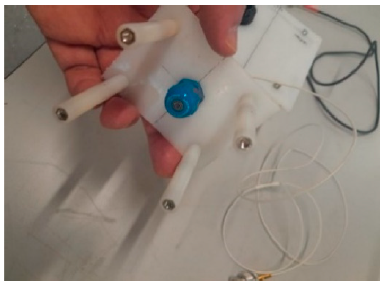
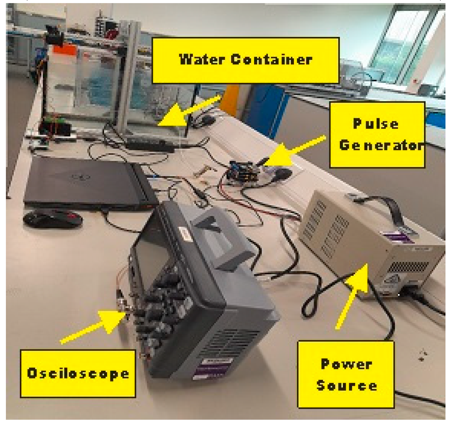
The experimental procedure used the XMS-310 cylindrical sensor, with a 10 MHz bandwidth and 3 mm diameter, to examine samples within a water containment system, as shown in Figure 1 and Figure 2.

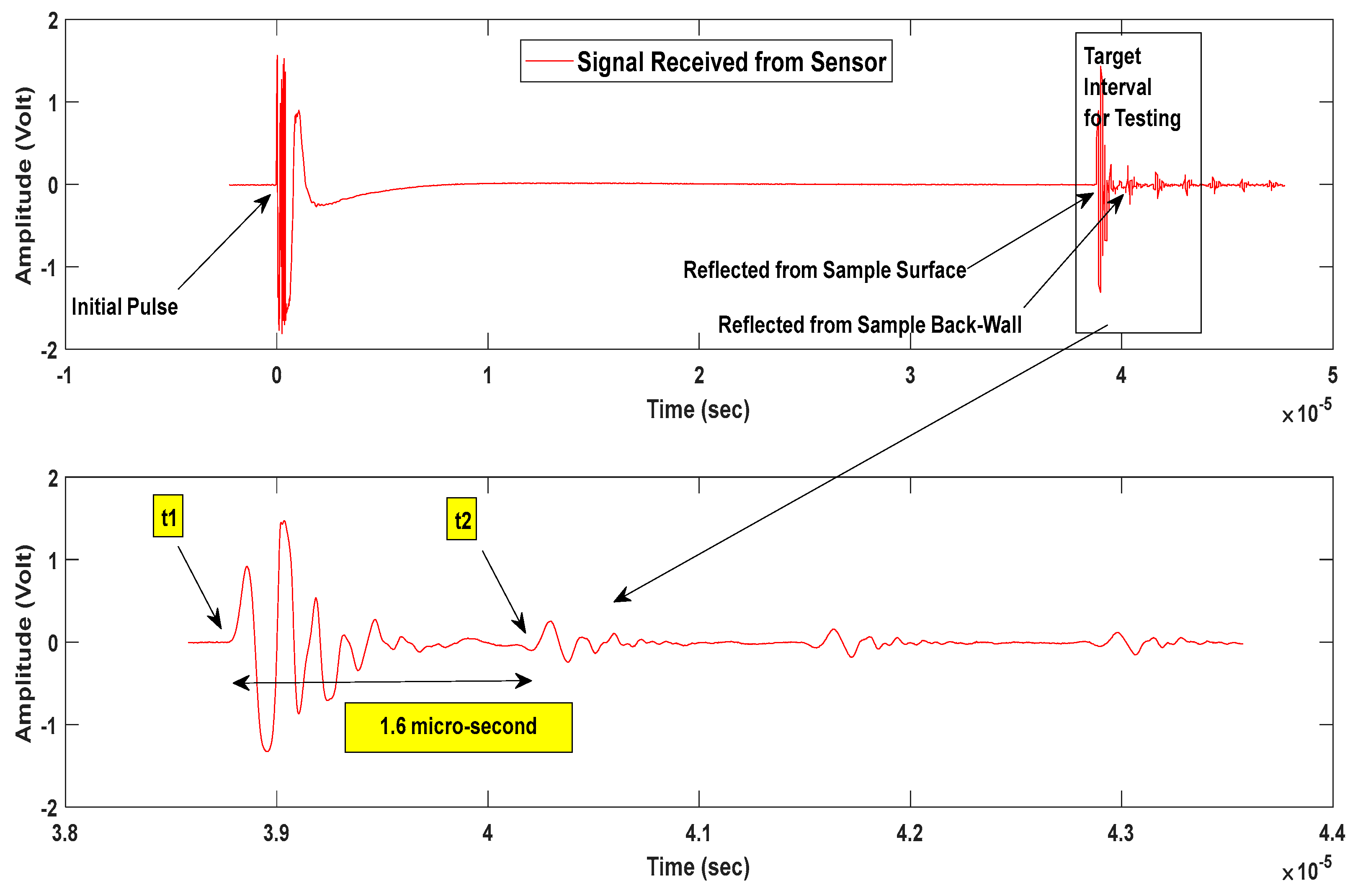
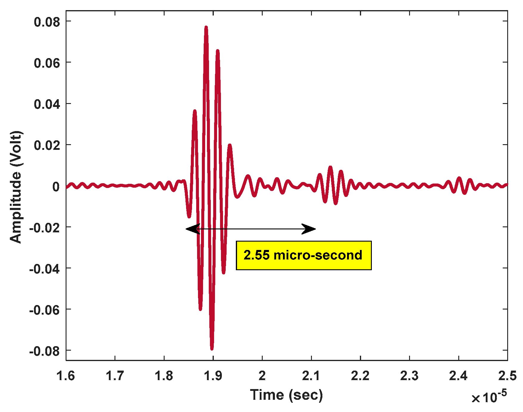
Figure 2 illustrates the non-contact ultrasonic experiment setup within a water container, where a pulse generator sends pulses to the sensor, a power source energizes the pulse generator, and an oscilloscope records and displays the waveform of the ultrasonic signal for analysis.

To accurately identify the peaks and valleys within the waveform, it is essential to define the following key points:

Initial Valley: This point represents the initiation of the ultrasonic pulse emission.
Second Valley: This point represents the initial reflection of the ultrasonic pulse from the surface of the sample.
Third Valley: This point indicates the reflection of the ultrasonic pulse after it has passed through the sample and returned to the sensor from the back wall.

These key junctures are depicted in Figure 4 across two separate plots.

2.1. Non-Contact Test Under the Water

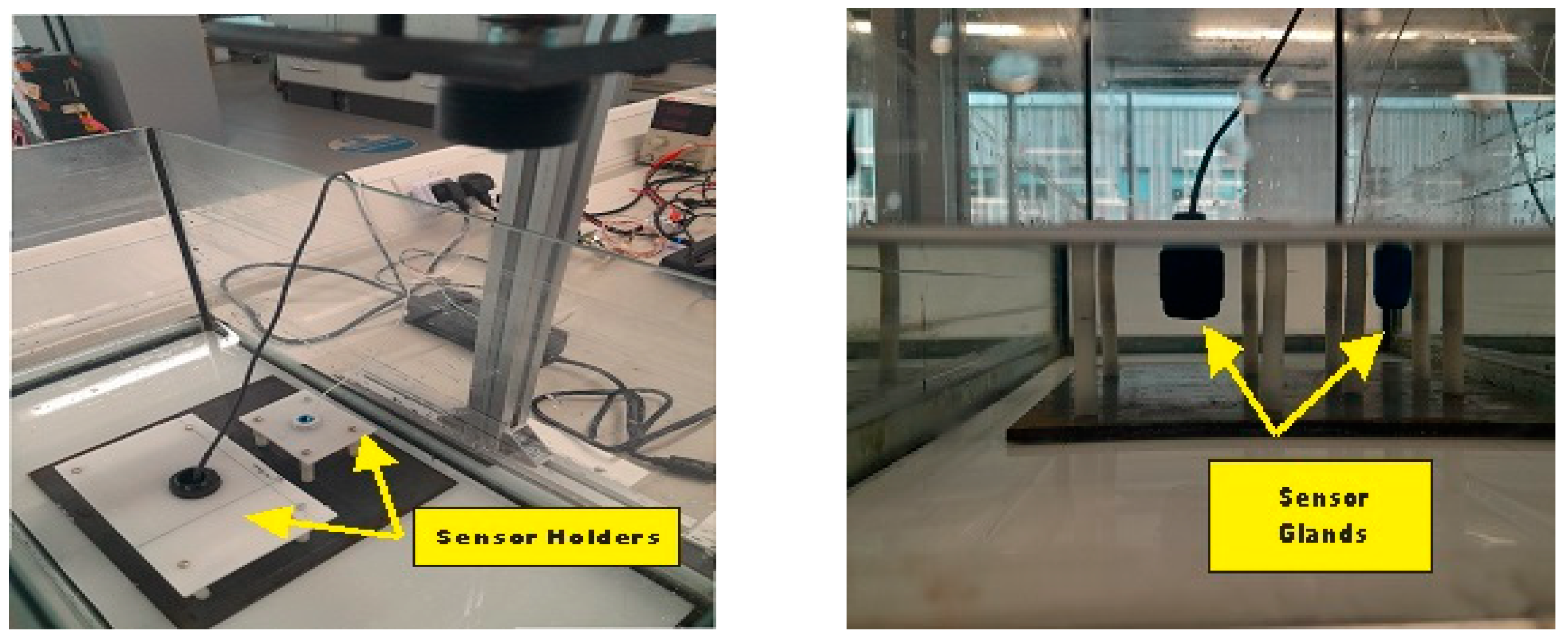
The ultrasonic sensor emits a pulse that travels through the water, enters the steel sample, and reflects back to the sensor, with Figure 3 displaying the sensor holders designed to keep the sensor submerged and stable at a constant distance from the sample's surface.

The experiment accounts for the additional distance the ultrasonic pulse travels through the water-filled gap before and after interacting with the steel sample, with the following section detailing the methodology for accurately calculating both the water gap and sample thickness:

a): Measure Time Intervals: Record the time intervals (referred to as t₁ and t₂) between the critical points present within the oscilloscope waveform, as explained previously. In Fig. 4, both t₁ and t₂ are indicated for the responses captured from the sensor.
b): Calculate Water Gap Distance: Using the measured time interval (t₁), we are able to calculate the distance (D_W) travelled by the ultrasonic pulse through the water gap using the speed of sound in the water (V_W):

D_W = V_W × t₁/2

(1)

c): Calculate Effective Time of Flight (ToF): Determine the total time of flight of the ultrasonic pulse through both the water gap and the steel sample:

t_total = t₂ – t₁

(2)

d): Calculate Thickness: Finally, use the effective ToF through the steel (t_S) to calculate the thickness (T) of the steel sample using the speed of sound in steel (V_S):

T = V_S × (t_total) / 2

(3)

Where:

T = Thickness of the steel sample
V_W = Speed of sound in water (1500 m/s)
V_S = Speed of sound in steel (5920 m/s)
t₁ = Time taken for the ultrasonic pulse to travel from the sensor to the water-steel interface (sec)
t₂ = Time taken for the ultrasonic pulse to travel from the sensor to the second reflection (sec)
D_W = Distance travelled by the ultrasonic pulse through the water gap (meters)
t_total = Total ToF of the ultrasonic pulse through the steel sample (sec)

2.1. Wedge Test

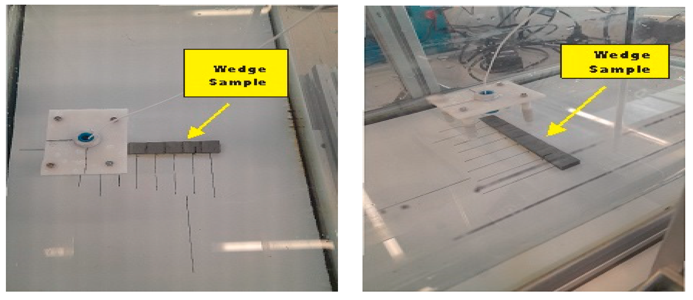
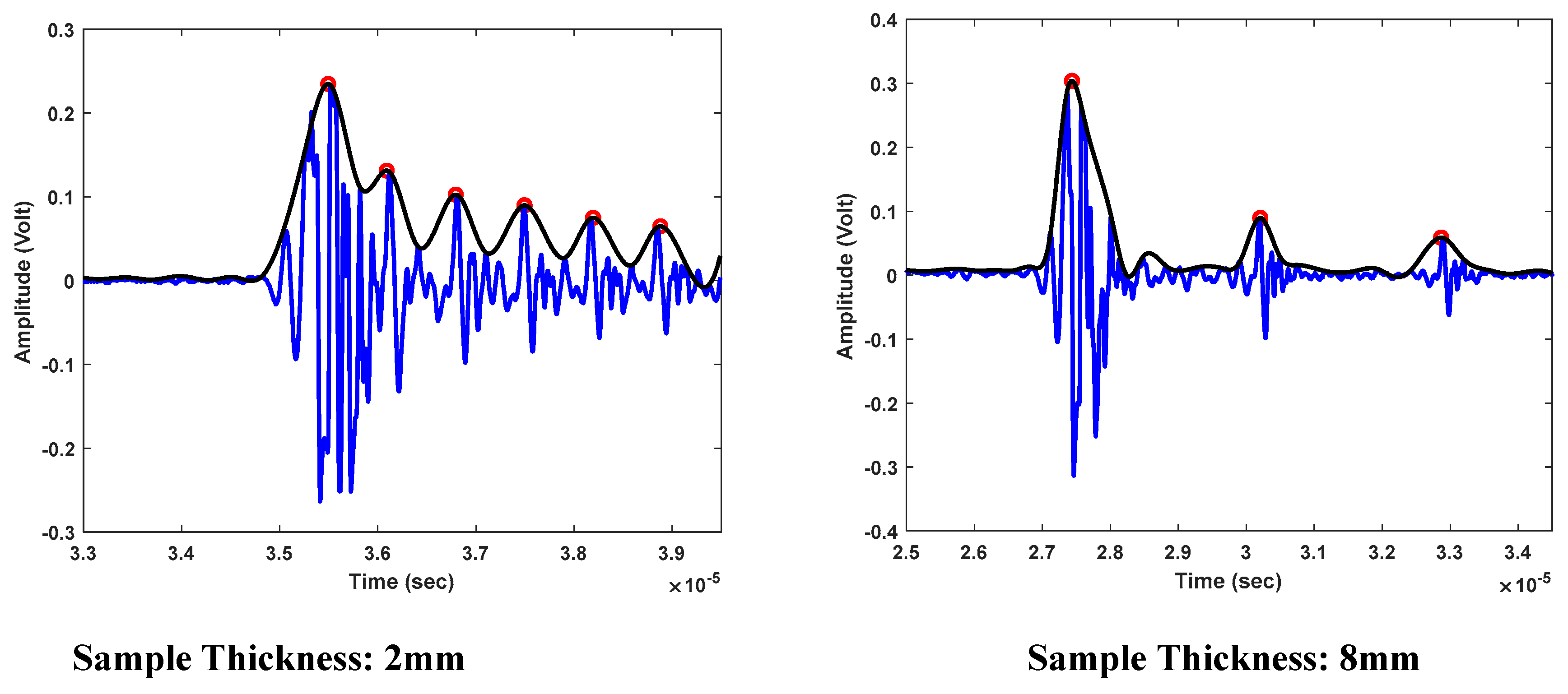
The sensor's performance was evaluated using a wedge of varying thicknesses (2 mm to 8 mm), as shown in Figure 5, with the results in Table 1 revealing minimal discrepancies between the sensor's measurements and the actual wedge thicknesses, indicating high accuracy.

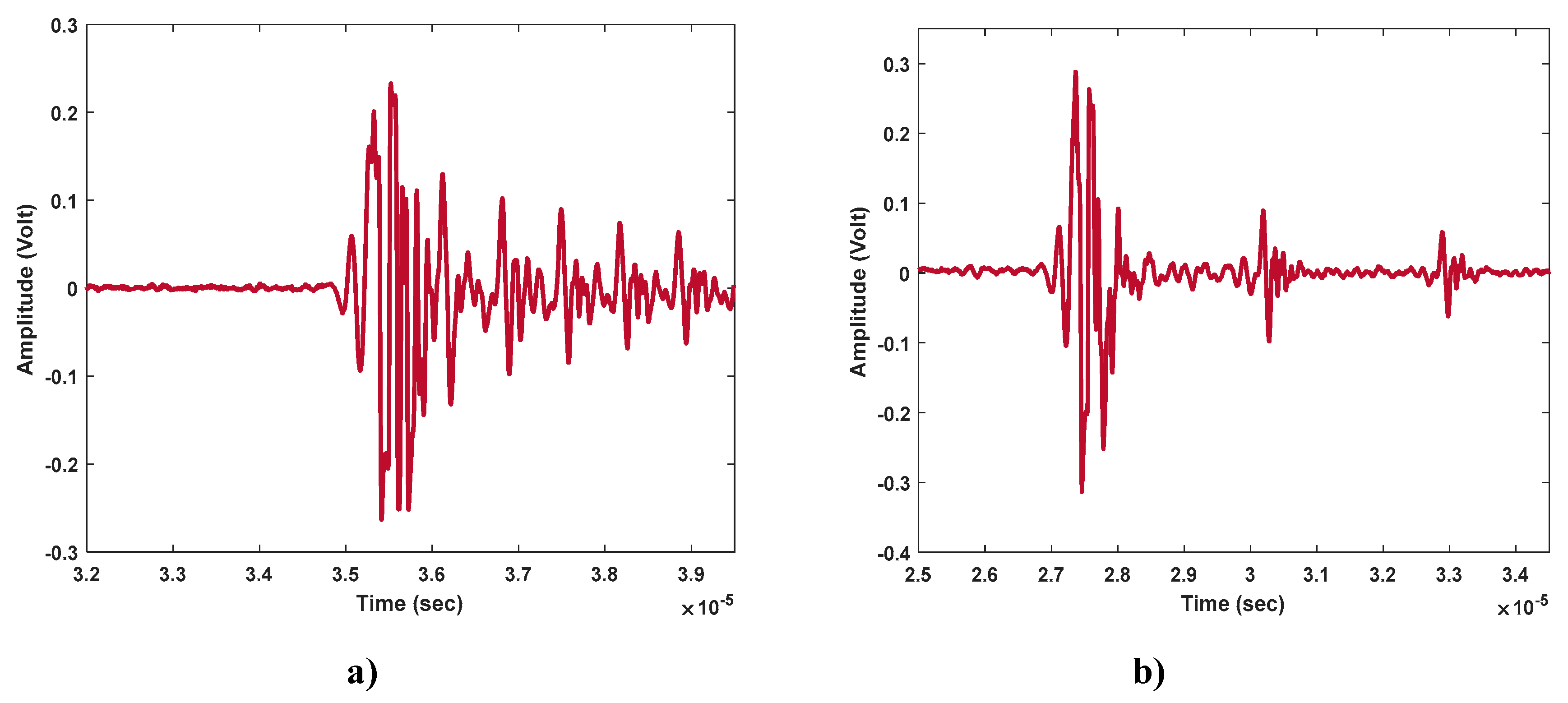
Figure 6 shows the plots obtained for the different thicknesses of the wedge.

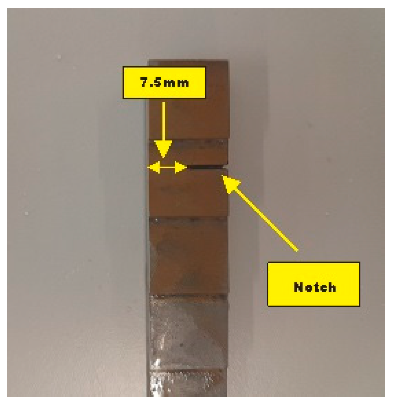
A groove, located 7.5 mm from the top edge of the wedge as shown in Figure 7, has been integrated to measure the Depth of Displacement (DoD) within the sample using the sensor.

The Depth of Displacement (DoD) of the notch, measured by positioning the sensor at the top edge of the wedge, was estimated at 7.6 mm, showing minimal measurement error, with the data presented in Figure 8.

DoD Prediction by Using Recommender System

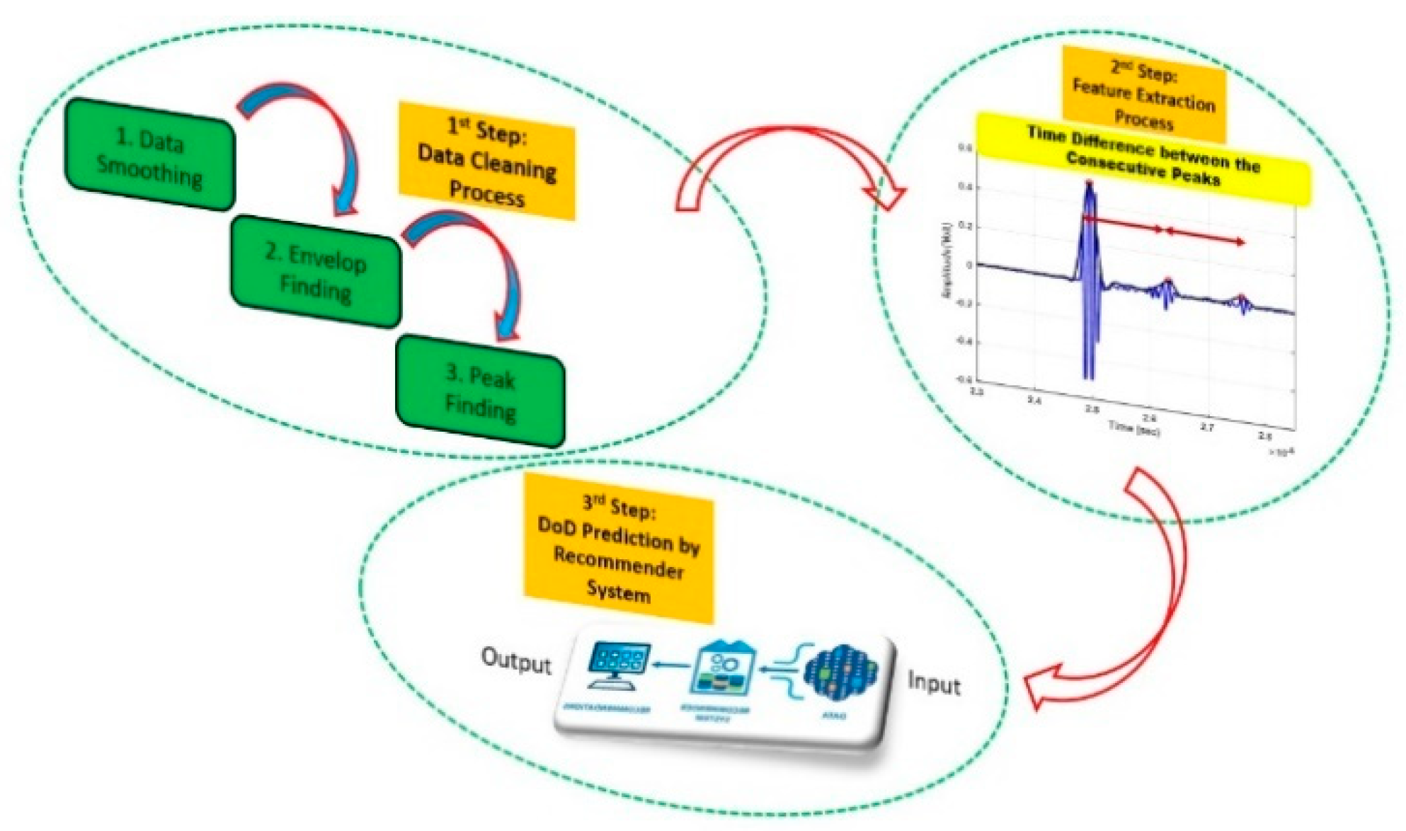
This section outlines a three-phase methodology for predicting Depth of Displacement (DoD) in the test sample, involving data preprocessing, feature extraction, and DoD forecasting via a recommender system, with detailed signal cleaning, smoothing, enveloping, and peak detection techniques described in subsections 3.1 through 3.3.

3.1. Data Smoothing by using Moving Average Algorithm

In the moving average algorithm, when provided with a time-series signal as input,

X_{n}

with length, N, where n = 0, 1, 2, ..., N-1, we have the ability to determine and specify the size of the moving average window as M, which corresponds to the number of neighbouring samples that are taken into account for the purpose of smoothing. The moving average algorithm is described taking the following steps:

1. Initialize the smoothed signal

y_{n}

as an array consisting of zeros, where the length of the array matches that of the input signal

X_{n}

2. For each sample index n from M/2 to N - M/2 (both inclusive), calculate the moving average for the current index of the sample using the following relationship:

y_{n} = \frac{1}{M} \sum X_{n - \frac{M}{2} + K}, where K = 0, 1, 2, \dots, M - 1

(4)

3. For sample indices outside the range M/2 to N - M/2, we have the option to either add zero-padding to the signal or adjust the range accordingly in order to accommodate the available samples.

4. The resulting smoothed signal

y_{n}

represents the moving average of the original signal

X_{n}

It is essential to note that this mathematical representation assumes a symmetric moving average window, where an equal number of samples is taken into account on both sides of the current sample.

3.2. Envelop Finding Algorithm

The mathematical notation below outlines the algorithm for determining the envelope of a time-series signal. When provided with a time-series signal as input,

X_{n}

with length N, where n = 0, 1, 2, ..., N-1, the following steps are taken:

It is recommended to apply this algorithm after performing pre-processing steps, such as smoothing or filtering, on the input signal, $X_{n}$ to reduce noise, fluctuations and also obtain more reliable results.
Calculate the upper envelope of the signal, which corresponds to the maximum values at each time point. Let's denote the upper envelope as $U_{n}$ .

Initialize $U_{n}$ as an array of zeros with the same length as $X_{n}$ .
For each sample index n from 1 to N-2, perform the following steps:

If $X_{n}$ is greater than both $X_{n - 1}$ and $X_{n + 1}$ , set $U_{n}$ equal to $X_{n}$ .
Otherwise, set $U_{n}$ equal to the maximum value between $U_{n - 1}$ and $U_{n + 1}$ .

c.: For the sample indices n = 0 and n = N-1, set $U_{n}$ equal to the maximum value between $U_{n + 1}$ and $U_{n - 1}$ , respectively.

It is essential to note that this mathematical representation applies for a discrete-time signal.

3.3. Peak Finding Algorithm

The mathematical formalism below outlines the algorithm for identifying peaks in the envelope of a time-series signal. Given an input envelope signal

E_{n}

of length N, where n = 0, 1, 2, ..., N-1, the following steps are taken:

Set a threshold value, denoted as T, which represents the minimum amplitude difference necessary to detect a peak.
Create an empty array to store the indices of the identified peaks, P.
For each sample index n from 1 to N-2, if $E_{n}$ is greater than both $E_{n - 1}$ and $E_{n + 1}$ by at least the threshold T, add n to the array P as a detected peak.
The array P contains the indices of the detected peaks in the envelope signal $E_{n}$ .

Similarly, it is important to note that this algorithm applies for a discrete-time signal and requires the presence of an envelope signal.

3.4. Depth of Defect (DoD) Prediction by Recommender System

Recommender systems use algorithms like collaborative filtering, content-based filtering, and hybrid approaches, leveraging machine learning and data mining to analyze user data and generate personalized recommendations, as seen in e-commerce platforms where they suggest products based on users' past purchases and browsing history.

Recommender systems are essential in media platforms for creating personalized playlists and recommending movies or TV shows based on viewing habits, enhancing user engagement and retention, and with advancements in AI and big data, they have the potential to revolutionize decision-making, impacting user satisfaction and business performance [29].

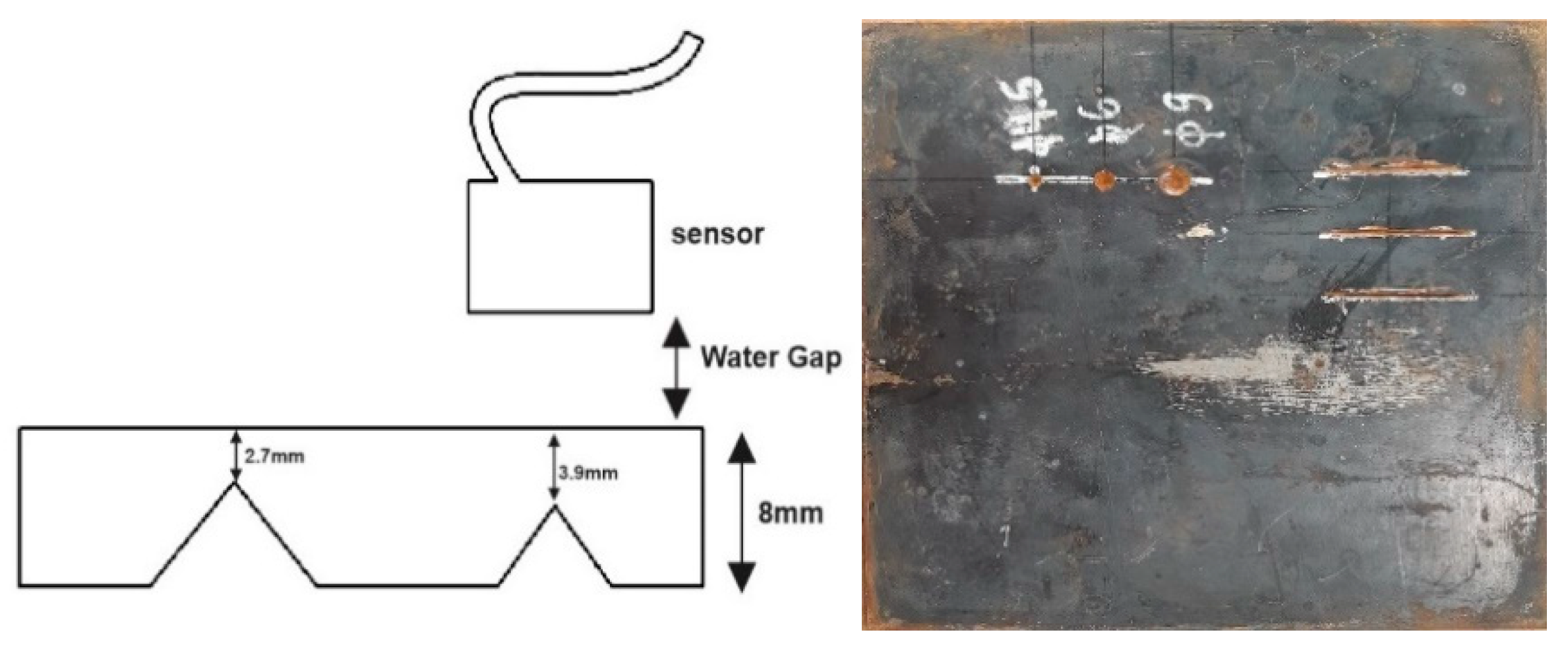
This section uses a recommender system based on an exponential function to predict the depth of defects in a sample with two drilled holes positioned 2.7mm and 3.9mm from the top surface, highlighting the capabilities of recommender systems in data analysis and inference.

Figure 10. Test Sample with the Two Predetermined Drilled Holes.

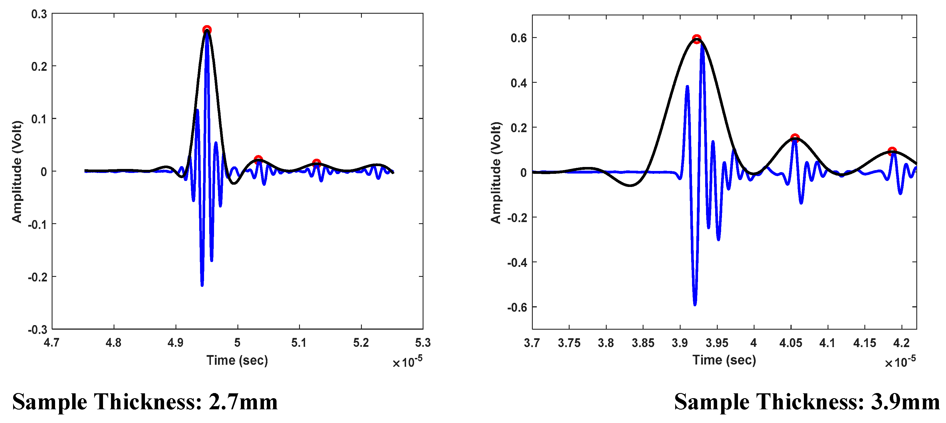
Following peak identification in Section 3.3, the time difference between consecutive peaks is used as the input feature vector for the recommender system to assess similarity between data from the wedge sample and the test sample with two predetermined voids, as shown in the workflow diagram (Figure 11) and similarity curves (Figure 12).

The similarity assessment is performed using an exponential function written as follows,

S (W_{i}, T_{j}) = e^{(- {(y_{w} - y_{t})}^{T} . (y_{w} - y_{t}))}

(5)

Where:

$S (W_{i}, T_{j})$ = Similarity function between wedge sample (W) and the test sample (T)
y_w - y_t = The corresponding vectors of the time difference between consecutive peaks of the wedge sample (y_w) and the test sample (y_t)

The subscript "i" in Equation (5) denotes the vectors of the wedge sample. For instance, "i=2" signifies the time differences between the consecutive peaks (red dots in Fig. 9) within a specific time interval at the wedge sample with a thickness of 2mm. The subscript "j" in Equation (5) represents the position of the hole at test sample from its top surface. For example, "j=1" denotes the time differences between the consecutive peaks (red dots in Fig. 12) within a specific time interval at the test sample with a thickness of 2.7mm from its top surface. The similarity percentages between the thicknesses of the wedge samples, namely 2mm, 3mm, 4mm, 5mm, 6mm, 7mm, and 8mm, are compared with the positions of the drilled holes at the test sample, i.e., 2.7mm and 3.9mm, using Equation (5). The results are displayed in Table 2 and Table 3. As an example, in these tables, S(W₂,T₁) denotes the similarity between the wedge sample with 2mm thickness and the void located at 2.7mm from the top surface of the test sample. Similarly, S(W₄,T₂) represents the similarity between the wedge sample with 4mm thickness and the void located at 3.9mm from the top surface of the test sample.

To estimate the depth of defects from the top surface of the test sample, the following equations are used for the voids located at 2.7mm and 3.9mm from the top, respectively:

t_{2.7 m m} = \frac{\sum_{i = 2}^{8} S (W_{i}, T_{1}) \times W_{i}}{\sum_{i = 2}^{8} S (W_{i}, T_{1})}

(6)

t_{3.9 m m} = \frac{\sum_{i = 2}^{8} S (W_{i}, T_{2}) \times W_{i}}{\sum_{i = 2}^{8} S (W_{i}, T_{2})}

(7)

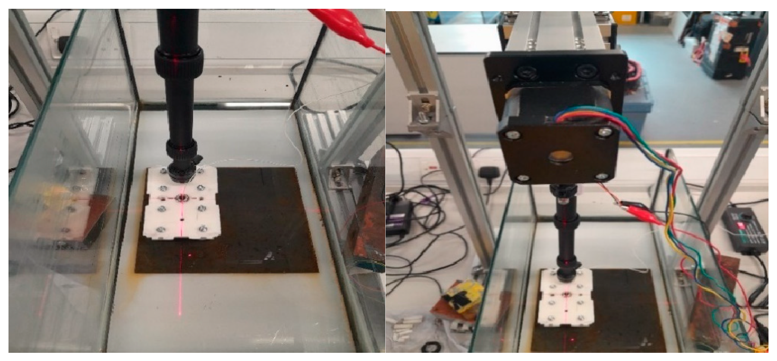
In equations (6) and (7), W_i denotes the thicknesses of the wedge sample. E.g., W₄ represents 4mm thickness. Using equations (6) and (7), two values were estimated for the locations of the voids from the top surfaces of the test sample, which are 2.75mm and 3.99mm, respectively. As seen in Table. 4, the predicted positions demonstrate a good agreement with the nominal positions. The curves in Fig. 12 were generated by a mobile platform and an installed laser pointer on it which is shown in Fig. 13.

4. Results and Discussion

This study develops a systematic feature extraction methodology and a recommender system for steel samples with specific geometrical properties, though its applicability may be limited to this material type and geometry, with the goal of demonstrating the approach's feasibility and accuracy for this specific material and paving the way for future research to extend the method to a wider range of materials through new recommender system architectures.

In spite of the limitations mentioned above, the results demonstrated an acceptable level of agreement between the nominal thickness values and the predicted DoDs by using the recommender system. As displayed in tables 2 and 3, the recommender system has demonstrated high accuracy in estimating the void locations relative to the sample's top surface. For instance, regarding the void positioned at 2.7mm from the top, the similarity values of S(W₂,T₁) and S(W₃,T₁) exhibited 70% and 80%, respectively, indicating that the void location lies between 2mm and 3mm from the top. Interestingly, a higher value was recorded for S(W₃,T₁) that indicates the void is closer to value of 3mm rather than 2mm. Similarly, regarding the void located at 3.9mm from the sample's top surface, the similarity values of S(W₃,T₂) and S(W₄,T₂) exhibited 87% and 99%, respectively, showing that the void location falls between 3mm and 4mm from the top. Notably, S(W₄,T₂) yielded a higher value that proves the void is closer to 4mm rather than 3mm.

5. Conclusions

In conclusion, this research successfully integrated ultrasonic sensors with recommender systems to predict Depth of Displacement (DoD), demonstrating that the proposed methodology provides non-invasive, real-time, and highly accurate results through time-series analysis and predictive modeling, thereby advancing real-time monitoring and showcasing the potential for combining these technologies in non-destructive testing and quality control.

Funding

This work has received funding from the EU’s Horizon Europe research and innovation programme, under grant agreement No. 101070115 (TUBERS project). Special thanks to all members of Essex.AI, and University of Essex for providing the research expertise and support for this research.

Conflicts of Interest

No conflict of interests.

References

D. K. Hsu, M. S. Hughes, Simultaneous Ultrasonic Velocity and Sample Thickness Measurement and Application in Composites, The Journal of Acoustical Society of America, 92(2) (1992) 669-675, . [CrossRef]
V. Hassani, T. Tjahjowidodo, A Hysteresis Model for A Stacked-Type Piezoelectric Actuator, Journal of Mechanics of Advanced Materials and Structures, 24 (2017) 73-87, . [CrossRef]
V. Hassani, T. Tjahjowidodo, Integrated Rate and Inertial Dependent Prandtl-Ishlinksii Model for Piezoelectric Actuator, 2^nd International Conference on Instrumentation Control and Automation, (2011) 35-40, . [CrossRef]
Ultrasound and Ultrasonic Testing, Iowa State University, Centre for Non-Destructive Evaluation, https://www.nde-ed.org/NDETechniques/Ultrasonics/Ultrasound.xhtml.
M. T. Shomalinasab, S. Sodagar, FE-based Ultrasonic Evaluation of HDPE Butt Fusion Joints, Journal of Nondestructive Testing Technology, 3 (2) (2023) 16-26, http//doi.org/ 10.30494/JNDT.2023.390294.1114.
J. Shah, S. El-Hawwat, H. Wang, Guided Wave Ultrasonic Testing for Crack Detection in Polyethylene Pipes: Laboratory Experiments and Numerical Modelling, Journal of Sensors, 23 (11) (2023), . [CrossRef]
N. Chidambaram, Ultrasonic Non-Collinear Shear Wave Mixing for the Detection of Ageing in PVC Pipes, Master Thesis, University of Twente, (2018), https://purl.utwente.nl/essays/75178.
D.-H. Koo, S. T. Ariaratnam, Innovative Method for Assessment of Underground Sewer Pipe Condition, Journal of Automation in Construction, 15 (2006) 479-488, . [CrossRef]
R. A. Gómez, M. S.- Silva, F. Muñoz, F. Schoefs, E. B.- Arteaga, Spatial Characterization and Simulation of New Defects in Corroded Pipeline based on In-Line Inspections, Journal of Reliability Engineering and System Safety, 241 (2024) 109697, . [CrossRef]
G. Acciani, G. Brunetti, G. Fornarelli, A. Giaquinto, Angular and Axial Evaluation of Superficial Defects on Non-Accessible Pipes by Wavelet Transform and Neural Network-based Classification, Journal of Ultrasonics, 50 (2010) 13-25, https://doi:10.1016/j.ultras.2009.07.003.
D. Santos, M. A. Machado, J. Monteiro, J. P. Sousa, C. S. Proença, F. S. Crivellaro, L. S. Rosado, T. G. Santos, Non-Destructive Inspection of High Temperature Piping Combining Ultrasound and Eddy Current Testing, Journal of Sensors, 23 (2023), . [CrossRef]
C. Dumrongkit, M. Noipitak, C. Chiablam, C. Chiablam, Investigation of Transfer Correction for In-Service Inspection of Coated Steel Welds using Ultrasonic Method, Journal of Renewable Energy and Smart Grid Technology, 18 (1) (2023) 14-28, https://ph01.tci-thaijo.org/index.php/RAST/article/view/251085.
X. Xu, H. Jin, S. Wu, E. Wu, K. Yang, H. Wu, A Novel Method for Nozzle-to-pipe Weld Inspection from the Nozzle Side, IEEE International Ultrasonics Symposium (IUS), (2023) 1-4, . [CrossRef]
L. S. Dai, Q. S. Feng, X. Q. Xiang, J. Sutherland, T. Wang, D. P. Wang, Z. J. Wang, Application of USCCD on Girth Weld Defect Detection of Oil Pipelines, Journal of Applied Sciences, 10 (2020), . [CrossRef]
D. A. Ramatlo, D. N. Wilke, P. W. Loveday, A Data-Driven Hybrid Approach to Generate Synthetic Data for Unavailable Damage Scenarios in Welded Rails for Ultrasonic Guided Wave Monitoring, Journal of Structural Health Monitoring, (2023) 1-24, . [CrossRef]
F. Yang, D. Shi, L.-Y. Lo, Q. Mao, J. Zhang, K.-H. Lam, Auto-Diagnosis of Time-of-Flight for Ultrasonic Signal Based on Defect Peaks Tracking Model, Journal of Remote Sensing, 15 (3) (2023), . [CrossRef]
C. Cirtautas, V. Samaitis, L. Mažeika, R. Raišutis, Detection and Classification of Uniform and Concentrated Wall-Thinning Defects Using High-Order Circumferential Guided Waves and Artificial Neural Networks, Journal of Sensors, 23 (2023), . [CrossRef]
C. Y. Teoh, J. S. Pang, M. N. Abdul Hamid, L. E. Ooi, W. H. Tan, Ultrasonic Guided Wave Testing on Pipeline Corrosion Detection using Torsional T(0,1) Guided Waves, Journal of Mechanical Engineering and Sciences (JMES), 16 (4) (2022) 9157-9166, . [CrossRef]
D. Cirtautas, Corrosion-Based Defect Detection and Classification in Pipe Wall Using Multiple High Order Ultrasonic Guided Wave Modes, 13^th European Conference on Non-Destructive Testing (ECNDT 2023), 28 (8) (2023), https://www.ndt.net/?id=28436.
M. McInnes, C. Dick, C. Thring, D. Irving, D. Hughes, Flexible, Scalable, Printed Ultrasound Sparse Array for Corrosion Detection using Machine Learning, IEEE International Ultrasonics Symposium (IUS), (2023), . [CrossRef]
S. Iyer, S. K. Sinha, M. K. Pedrick, B. R. Tittmann, Evaluation of Ultrasonic Inspection and Imaging Systems for Concrete Pipes, Journal of Automation in Construction, 22 (2012) 149-164, . [CrossRef]
D. Peng, F. Cheng, X. She, Y. Zheng, Y. Tang, Z. Fan, Three-Dimensional Ultrasonic Reverse-Time Migration Imaging of Submarine Pipeline Nondestructive Testing in Cylindrical Coordinates, Journal of Marine Science and Engineering, 11 (7) (2023), . [CrossRef]
F. Bettayeb, T. Rachedi, H. Benbartaoui, An Improved Automated Ultrasonic NDE System by Wavelet and Neuron Networks, Journal of Ultrasonics, 42 (2004) 853-858, . [CrossRef]
J.D. Eckels, E.M. Jacobson, I.T. Cummings, I.F. Fernandez, K. Ho, N. Dervilis, E.B. Flynn, A.J. Wachtor, Predicting Local Material Thickness from Steady-State Ultrasonic Wavefield Measurements Using A Convolutional Neural Network, Journal of Ultrasonics, 123(2022) 106661, . [CrossRef]
C.C. Aggarwal, Neural Networks and Deep Learning: A Textbook, Springer International Publishing, ISBN: 9783319944630, (2018).
F. Cau, A. Fanni, A. Montisci, P. Testoni, M. Usai, Artificial Neural Networks for Non-Destructive Evaluation with Ultrasonic Waves in not Accessible Pipes, IEEE Industry Applications Conference, (2005), . [CrossRef]
Carvalho, J. M. A. Rebello, L. V. S. Sagrilo, C .S. Camerini, I. V. J. Miranda, MFL Signals and Artificial Neural Networks Applied to Detection and Classification of Pipe Weld Defects, Journal of NDT&E International, 39 (2006) 661-667, . [CrossRef]
Q. Ma, G. Tian, Y. Zeng, R. Li, H. Song, Z. Wang, B. Gao, K. Zeng, Pipeline In-Line Inspection Method, Instrumentation and Data Management, Journal of Sensors, 21 (11) (2021), . [CrossRef]
F. Ricci, L. Rokach, B. Shapira, Recommender Systems Handbook, Third Edition, Springer, ISBN 978-1-0716-2196-7, (2015), . [CrossRef]

Figure 1. Cylindrical Sensor with 3mm Diameter inside the Blue Gland (XMS-310 with 10 MHz bandwidth).

Figure 2. Experimental Set-up.

Figure 3. Left) Sensor Holder (Top-View), Right) Sensor Holder (Front-View).

Figure 4. Signal Received from the Sensor under the Water.

Figure 5. Left) Wedge Test (Top-View), Right) Wedge Test (Side-View).

Figure 6. a) 2mm, b) 8mm.

Figure 7. Notch on the Wedge, 7.5mm Distance from the Upper Edge of the Wedge.

Figure 8. Signal Reflected from the Notch.

Figure 9. Time Difference between the Consecutive Peaks Shown by Red Dots.

Figure 11. Workflow Diagram of the DoD Prediction Process.

Figure 12. Time Difference between the Consecutive Peaks Shown by Red Dots; Left) Signal for the Void Located at 2.7mm from the Top, Right) Signal for the Void Located at 3.9mm from the Top.

Figure 13. Left) Moving Set-up with Laser Pointer, Right) Step Motor to Move the Platform.

Table 1. Comparison between Measured Values by Sensor and the Nominal Values of Wedge Thicknesses.

Nominal Values (mm)	Measured Values by Sensor (mm)
2	2.04
3	2.98
4	3.99
5	5
6	6
7	6.98
8	7.99

Table 2. Similarity between Wedge Sample with Different Thicknesses and Hole in the Test Sample Located at 2.7mm from the Top.

S(W₂,T₁)	S(W₃,T₁)	S(W₄,T₁)	S(W₅,T₁)	S(W₆,T₁)	S(W₇,T₁)	S(W₈,T₁)
70%	80%	22%	2%	0	0	0

Table 3. Similarity between Wedge Sample with Different Thicknesses and Hole in the Test Sample Located at 3.9mm from the Top.

S(W₂,T₂)	S(W₃,T₂)	S(W₄,T₂)	S(W₅,T₂)	S(W₆,T₂)	S(W₇,T₂)	S(W₈,T₂)
45%	87%	99%	70%	35%	10%	2%

Table 4. Comparison between Measured Values by Sensor for the Locations of the Voids at the Test Samples and the Predicted Values by Recommender System.

Nominal Values (mm)	Predicted Values by Recommender System (mm)
2.7	2.75
3.9	3.99

Disclaimer/Publisher’s Note: The statements, opinions and data contained in all publications are solely those of the individual author(s) and contributor(s) and not of MDPI and/or the editor(s). MDPI and/or the editor(s) disclaim responsibility for any injury to people or property resulting from any ideas, methods, instructions or products referred to in the content.

© 2024 by the authors. Licensee MDPI, Basel, Switzerland. This article is an open access article distributed under the terms and conditions of the Creative Commons Attribution (CC BY) license (http://creativecommons.org/licenses/by/4.0/).

Copyright: This open access article is published under a Creative Commons CC BY 4.0 license, which permit the free download, distribution, and reuse, provided that the author and preprint are cited in any reuse.

Alerts

MDPI Initiatives

Important Links

Choose an area of interest and we will send you notifications of new preprints at your preferred frequency.

Disclaimer

Depth of Defect Detection in Immersive Environments through Ultrasonic Sensor Data Analysis and Recommender System

Abstract

Keywords:

Subject:

1. Introduction

2. Experimental Set-Up

2.1. Non-Contact Test Under the Water

2.1. Wedge Test

DoD Prediction by Using Recommender System

3.1. Data Smoothing by using Moving Average Algorithm

3.2. Envelop Finding Algorithm

3.3. Peak Finding Algorithm

3.4. Depth of Defect (DoD) Prediction by Recommender System

4. Results and Discussion

5. Conclusions

Funding

Conflicts of Interest

References

MDPI Initiatives

Important Links

Subscribe