1. Introduction
Time series classification methods based on deep learning have many applications in the field of remote sensing [
1], which can capture significant time dependencies and have better performance than earlier time series classification methods. However, they require a large number of labeled time-series samples for training. Acquiring the training set is an often daunting and expensive task. This challenge is magnified in time series classification by the intricate and high-dimensional characteristics of time series data [
4]. Active learning is a promising way for time series classification to select the most informative data for labeling to save human labeling effort [
2]. This approach can achieve higher model accuracy with fewer labeled samples to reduce labeling costs [
3] significantly.
In the field of remote sensing, numerous active learning methods focus on sample selection for hyperspectral remote sensing image data based on uncertainty or representativeness. For instance, [
5] proposed an active learning algorithm based on a weighted incremental dictionary learning, which selects training samples that maximize two selection criteria, namely representative and uncertainty. [
6] development of a new AL framework for deep networks, where an auxiliary deep network for the basic learner is constructed to learn the uncertainty of unlabeled samples. [
7] propose a novel AL technique for sparse representation classifier, where the query function is designed by combining uncertainty and representativeness criteria. [
8] proposed a new semi-supervised classification method named prototype and active learning network, which integrates deep learning, active learning based on uncertainty, and prototype learning into a framework.
Many active learning methods have been developed for remote sensing image data, but none are especially effective for time series data. This is because it is hard to evaluate the informativeness of a time series sample by existing methods. Constructing a closed-form probability model for time series classification is challenging, further compounded by the complexities of directly adapting existing selection methods to time series datasets. Some study, such as in reference [
9], designs an informativeness metric that considers the characteristics of time series data in defining their instance uncertainty and utility. However, this method does not apply to multispectral and voluminous time series remote sensing data because of its expensive time complexity.
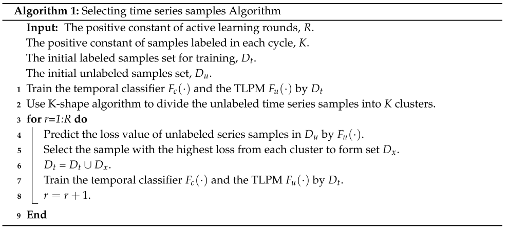
In this paper, we propose an effective active learning method for time series remote sensing image classification tasks, which aims to select informative time series data for training. This method selects samples based on both representativeness and uncertainty. For representativeness, we first address the metric by using the K-shape method to cluster time series samples. For uncertainty, we design a time-series loss prediction module(TLPM) that is equipped with a self-attention mechanism to predict classification loss and then select samples with high loss within each cluster. Finally, we conduct experiments on two temporal remote-sensing image datasets. Experimental results and ablation studies demonstrate the effectiveness of our method on time series data.
2. Methods
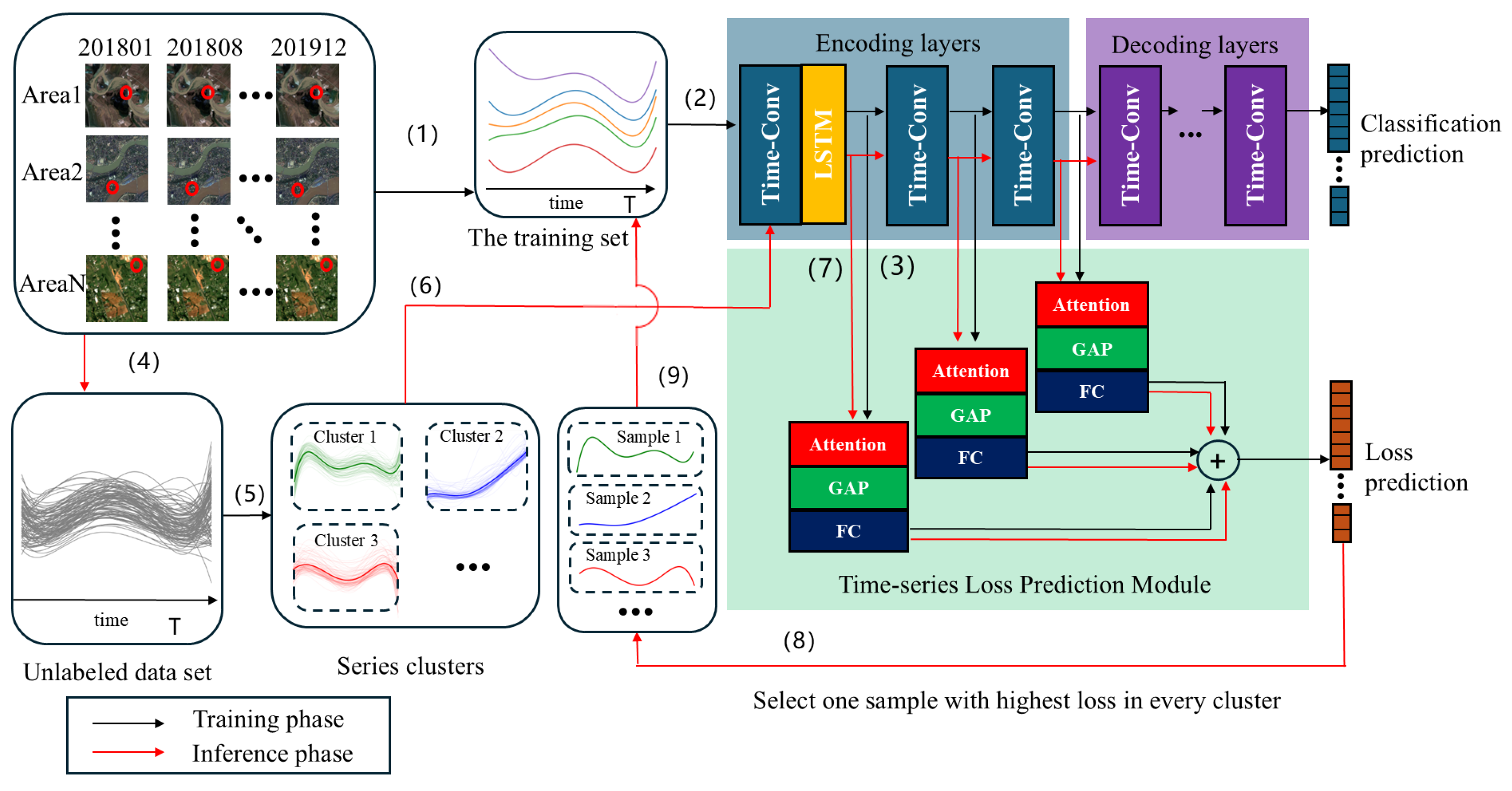
The active learning method proposed in this paper consists of three components: a clustering module, a temporal classifier, and the TLPM. The clustering module is the K-Shape method to provide support for selecting temporal samples from a perspective of sample representativeness. The time series classifier excels in time series classification because it can capture deep temporal dependencies. The TLPM predicts the loss of unlabeled temporal samples to evaluate the uncertainty of each time-series instance. The flowchart of the proposed method is displayed in
Figure 1. The process of sample selection comprises two main phases: training and referencing, which are performed in a loop. Before the loop starts, initial temporal samples are randomly sampled from a large dataset of remote-sensing images.
During the training phase, samples in the training set are inputted into the temporal classifier model for training. Simultaneously, the features extracted from the encoding section of the classifier are fed into the TLPM. The target loss from the temporal classifier is utilized as a label for training the TLPM.
During the inferencing phase, unlabeled data samples are first clustered, and the cluster labels are recorded. The next step is to input these samples into the temporal classifier and input the intermediate features into the TLPM. After that, we select time series samples with the highest loss in each cluster to label them and add them to the train set.
2.1. LSTM-Based Temporal Classifier
Time series data contains rich temporal information, which can be fully utilized for time series classification by a temporal classifier based on deep learning. Our classifier is based on the U-Net framework with an embedded LSTM layer. The convolutional layers in U-net can capture the temporal relationships of neighbor pixels over time. Meanwhile, the LSTM in this classifier captures long short-term temporal dependencies. This network has two advantages. Firstly, our network is a pure temporal version designed based on [
10], achieving outstanding performance with smaller and faster models. Secondly, an LSTM module added to the network can capture deep time dependencies and better filter out noise. The temporal classifier can be defined as
.
So far, this paper has introduced a temporal classifier that performs well on time series classification. However, it needs a large or well-selected training set. The reason is that a training set with a small data size is inadequate to support the classifier in accurately identifying the decision boundary between classes. Therefore, we propose an active learning method that considers representativeness and uncertainty to select informative samples to form a well-selected training set.
2.2. Select Samples Based on Representativeness and Uncertainty
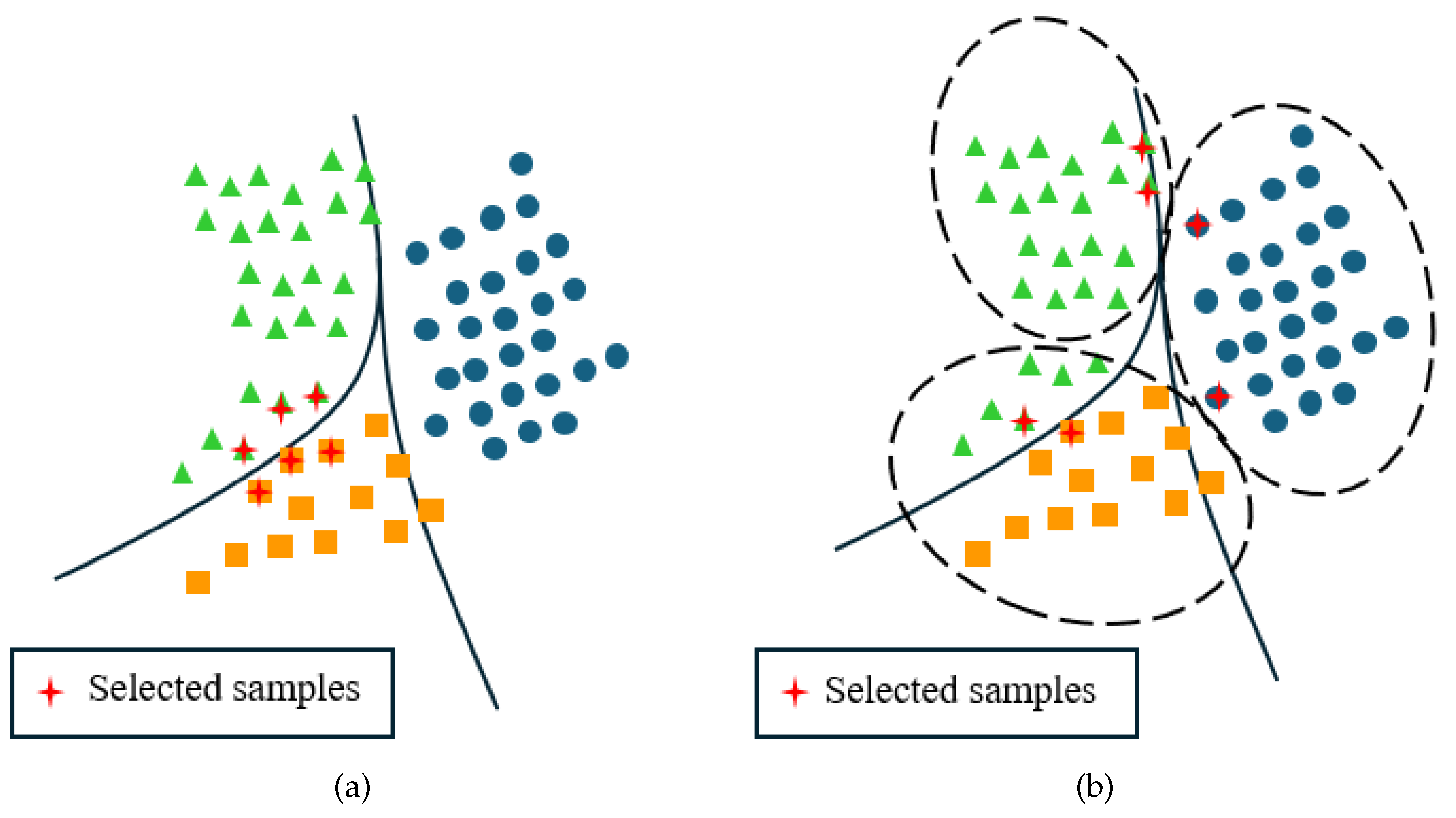
We commence with a crafted illustration highlighting the significance of selecting samples based on both representativeness and uncertainty in active learning.
Figure 2(a) shows the data selected by an approach based on uncertainty. The method based on uncertainty can find the decision boundary. But it is more likely to select similar samples. Figure
Figure 2(b) shows the data selected based on both representativeness and uncertainty. Evidently, the approach integrating both representativeness and uncertainty proves more effective in delineating the precise decision boundary compared to relying solely on uncertainty. In terms of representativeness, selecting unlabeled data from different clusters can help find more representative samples. The K-Shape method [
12] can efficiently divide unlabeled time series data into
K clusters because of its relatively small computational complexity and focus on the shape of the time series. In terms of uncertainty, the greater the classification loss of a sample, the greater the uncertainty of the sample. Therefore, we propose the TLPM to predict the loss of the sample. After using the K-shape method to divide the unlabeled samples into
K clusters, we select the sample with the maximum loss value from each of the
K clusters. Finally, we label these samples and add them to the training set.
The input part of the TLPM comes from the output features of different levels of the classifier in the encoding stage. Each input feature map will enter this submodule and undergo a series of transformations, which are defined here as
. Therefore, this network module
can be defined as:
represents the m-th output feature of the encoder, while
stands for fully connected transformation. Unlike the network of [
13], the
here does not only include the GAP layer [
14] and fully connected (FC) layer; we have made modifications to it. As shown in
Figure 1,
consists of three parts.
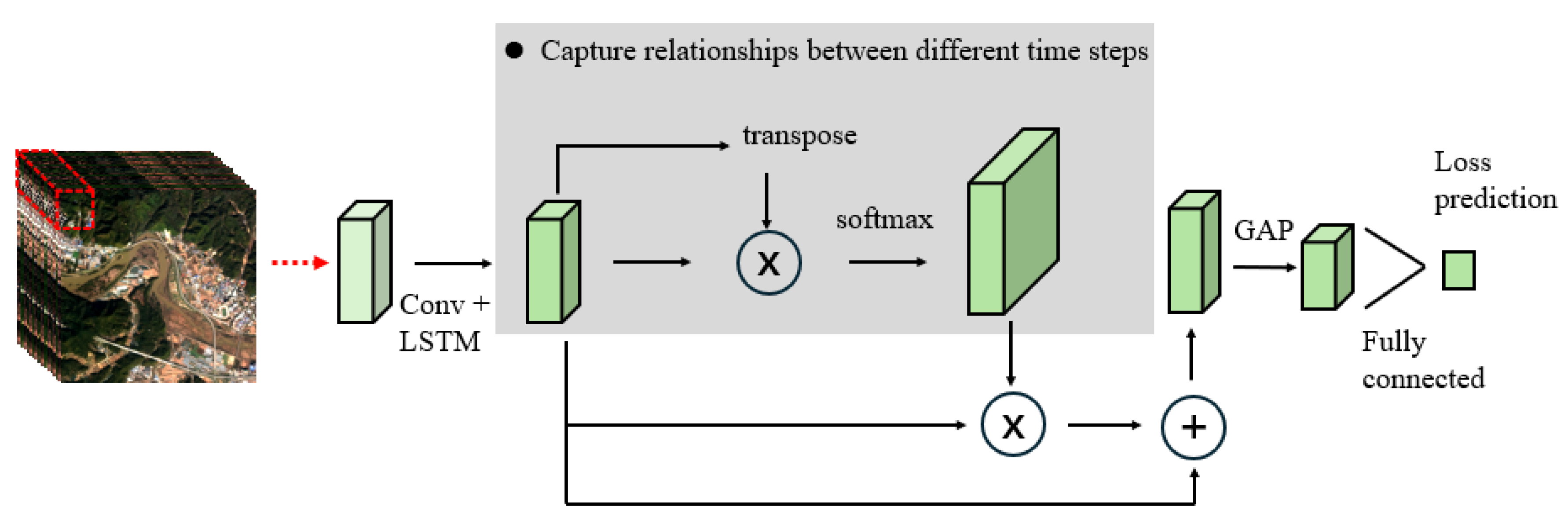
The first part involves a self-attention mechanism, which relates different positions of a single time sequence to compute a representation of the time sequence [
15]. As is shown in
Figure 3, it helps the module focus on the most critical time points when predicting the loss in time series data. The remaining two parts consist of the GAP and FC layers, respectively. Currently, we have not defined a specific loss function. In the next section, we will explain how to design the loss function and the method of training the network.
2.3. Loss Function of Our Network Architecture
In 2.1, we defined a temporal classifier for time series classification. In 2.2, we explained how to select time series samples based on the representativeness and uncertainty of the samples. Next, to enable the TLPM to accurately estimate the uncertainty of unlabeled data, we will define the loss function and explain the method of training the network. By inputting samples with labels into the classifier, we can obtain a loss value by comparing the true labels with the predicted ones. However, since unlabeled samples do not have corresponding labels, we cannot directly obtain the loss values for unlabeled data. Instead, we predict the loss value of a time-series instance through the TLPM. First, for the classifier, we define the output probability of
as
, so the loss value for a single sample
i is
represents the loss function of the classifier, where
is the true label of the sample and
. For the TLPM
, its predicted loss is denoted as
, and
is the corresponding actual loss value. Therefore, the loss of this module is defined as
. The total loss is defined as:
is an adjustable parameter used to represent a scaling constant in the loss optimization process. Specifically, for the classifier, we use cross-entropy loss as its loss function. When a batch contains
N temporal samples, the cross-entropy loss can be expressed as:
Defining the loss function for the TLPM is an important issue. During network training, while the classifier’s accuracy improves, its loss almost always decreases. It would be extremely challenging to train the TLPM using loss labels with large-scale variations. However, during network training, the relative loss values between temporal samples exhibit smaller variations. In other words, if we can compare loss functions between pairs of samples, we can discard the overall scale of loss. We designate a batch of trained data as
N, which is an even number. Thus, this batch contains
pairs of temporal sample data, denoted as
. We can then update the parameters of the TLPM by considering the difference between a pair of loss predictions, where the loss function is defined as:
Here, the symbol
represents a predefined positive number,
represents a pair of temporal samples
, and
represents the sign function. For example, when
and
, the loss function value is 0, providing no feedback to the network. Feedback from the loss values is received by the module only when
is larger than
and
, thereby increasing
and decreasing
. When the network trains a batch of data
with a size of
N, the final loss function for the classifier and the TLPM is represented as:
During training, the losses of both the classifier and the TLPM are simultaneously reduced. This means that the network parameters of these two modules are updated simultaneously, without requiring additional time or computational resources for separate steps.
3. Experiments and Results
3.1. Dataset and Experimental Environment
To validate the proposed method, we conducted experiments using two datasets: the two-class time series dataset named the multi-temporal urban development spacenet dataset (MUDS) [
17] and the multi-class time series dataset named DynamicEarthNet [
16]. The specific details can be seen in
Table 1. The methods proposed in this paper are compared with other methods on the two datasets, including random sampling, entropy sampling, and Variational Adversarial Active Learning(VAAL) [
11].
The experiments were run on an Intel(R) Xeon(R) Silver 4210 2.20-GHz CPU and an NVIDIA GeForce RTX 4090 GPU. The temporal classifier we employ is a one-dimensional temporal version based on the modification of BANet [
10]. Each input sample in the temporal sequence is of size 4x24, where 4 denotes the number of bands, and 24 represents the length of the sequence. The output size is 24xC, where C represents the initial category set during the initialization of the temporal classifier. In each dataset, we first perform uniform sampling with a stride of 4 along the spatial dimension of the original remote sensing images. Next, take 70% of the data as the test set, 10% of the data as the validation set, and from the remaining 20% of the data, select 100,1000 or 10000 samples as the initial training set, with the rest of the data as the candidate set. To prevent the problem of decreased accuracy in temporal classifiers caused by overfitting, during the training of the time-series classifier for 200 epochs, the network parameters that yield the highest accuracy on the validation set are chosen as the final parameters for the temporal classifier. The temporal classifier in this state is then used to test the accuracy of the final test set. To improve network training speed, a large batch size of 4096 was used. Parameters
and
were set to 1, and the fully connected layer had 64 neurons. To validate our method’s effectiveness, each approach was executed five times, and the average of their results was taken as the final accuracy.
3.2. Experiments on Two-Class Dataset
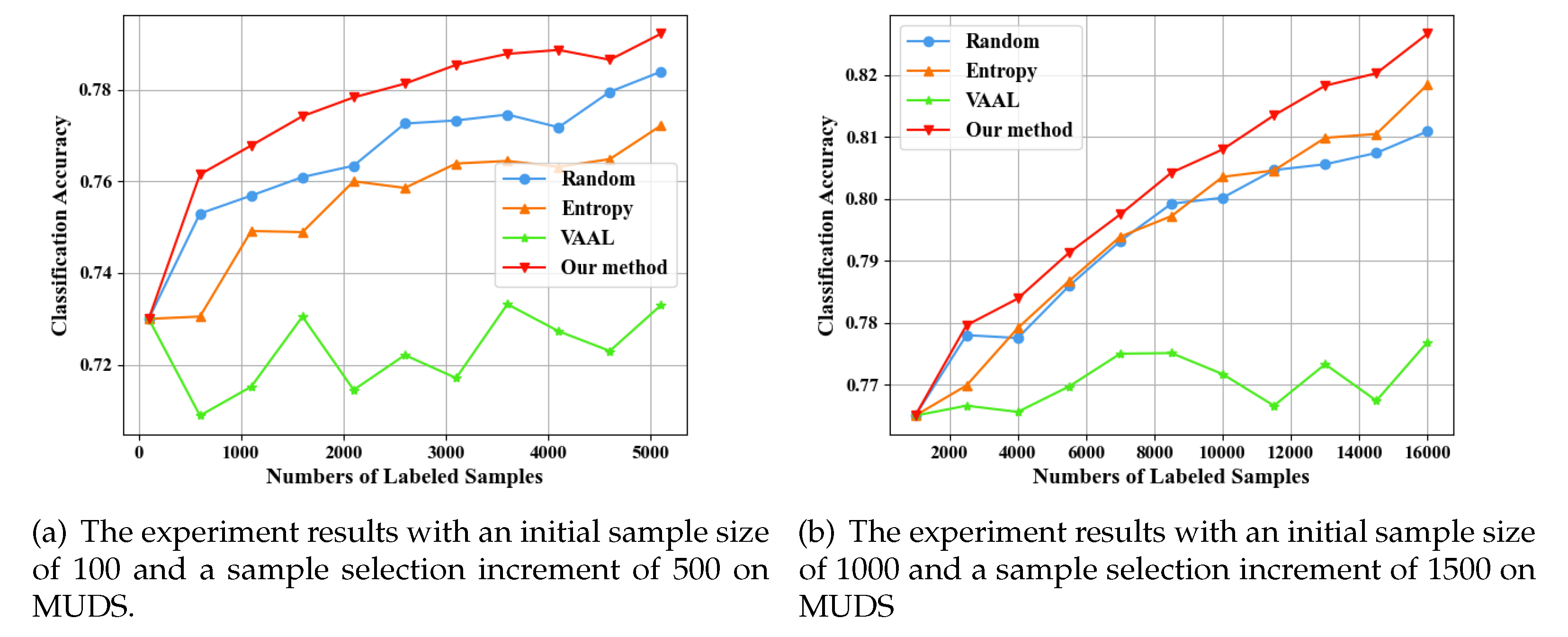
The two-class dataset used in this paper is MUDS. The experiment is divided into two groups. In the first group, the initial training set size is set to 100, and the sample selection interval is also set to 500 samples. In the second group, the initial training set size is set to 1000, with a sample selection interval of 1500. The initial learning rate for the temporal classifier is set to 0.01, and during training, the Adam optimizer adaptively adjusts the learning rate. The initial learning rate for the TLPM is also set to 0.01. After 90 epochs, the learning rate decreases to 0.001. During each training process, gradient propagation from the TLPM to the temporal classifier stops after the 120th epoch.
As shown in
Figure 4(a) and
Figure 4(b), when the initial training set size is 100, and the interval is also 500, our approach has significant advantages, and the random sampling performs relatively better compared to the other two methods. When the initial training set size is 1000, and the interval is 1500, the accuracy of the training set grows relatively steadily. Our method still performs well, and entropy sampling has also shown some effectiveness.
In general, the random method performs well when the data volume is small. This is because, with a smaller data volume, temporal classifiers have a limited understanding of the sample distribution, and randomly selected samples can provide more information to the temporal classifier. On the other hand, the entropy method does not perform well and sometimes yields worse results than the random method. This is because the entropy method itself selects too many similar samples, resulting in limited information for the temporal classifier, thus not significantly improving classifier accuracy. Our approach not only considers sample selection from the perspectives of representativeness and uncertainty but also selects samples with larger losses in time series based on these two aspects. Therefore, this approach significantly enhances the performance of the temporal classifier. The VAAL method performs poorly because it is challenging for the variational auto-encoder to encode and decode time samples with temporal dependencies.
3.3. Experiments on Multi-Class Dataset
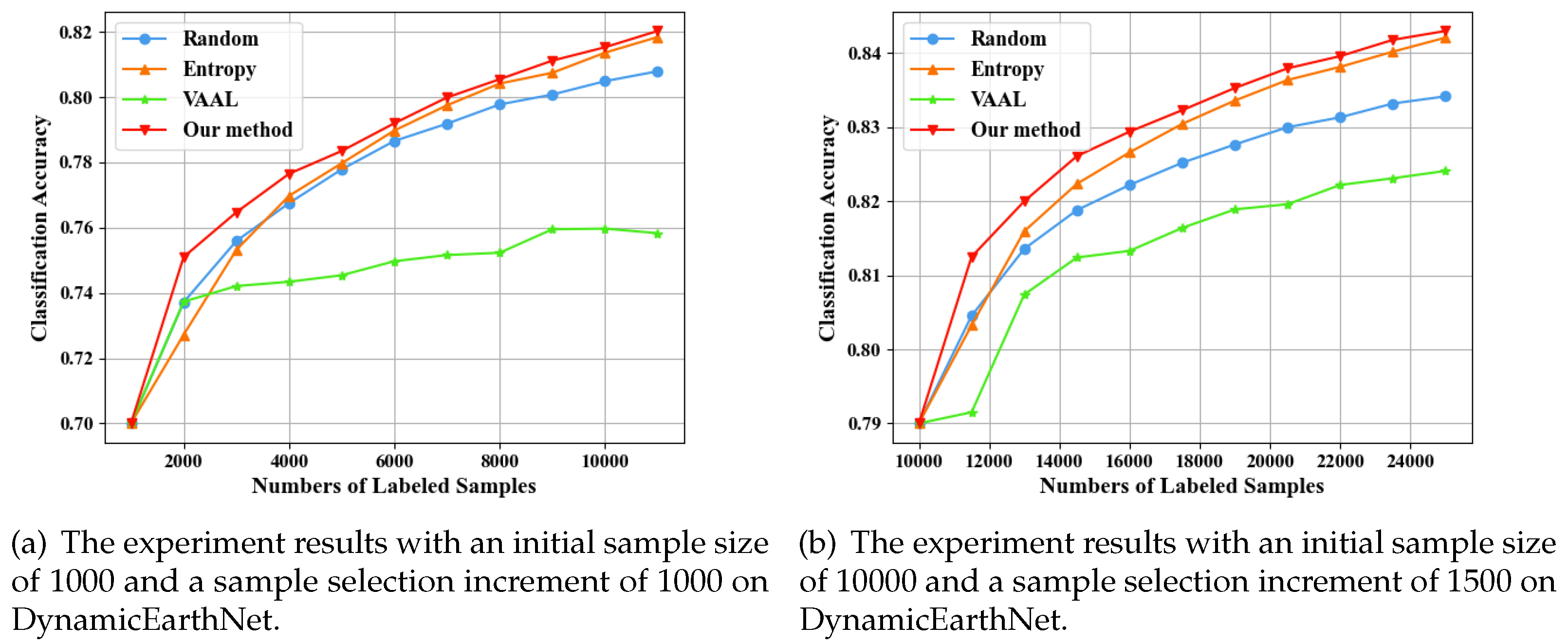
The experiments on DynamicEarthNet are divided into two groups. In the first group, the initial training set size is set to 1000, and the sample selection increment is set to 1000 samples. In the second group, the initial training set size is set to 10000, and the sample selection increment is set to 1500 samples. The initial learning rate of the temporal classifier is set to 0.01, and during training, the Adam optimizer adaptively adjusts the learning rate. The initial learning rate of the TLPM is set to 0.01, which decreases to 0.001 after 100 epochs. During each training process, gradient propagation from the TLPM to the temporal classifier stops after the 120th epoch. The difference from the MUDS experiment lies in the fact that the output of the temporal classifier used in this dataset has a category dimension of 7.
As shown in
Figure 5(a) and
Figure 5(b) in multi-class dataset, the performance of the random method initially surpasses that of the entropy method. However, the entropy method consistently overtakes the random method after several sample selections. The VAAL method performs worse than the random method. The method proposed in this paper shows a significant advantage, performing better than other active learning methods both within the sample quantity range of 1000 to 10000 and within the range of 10000 to 25000.
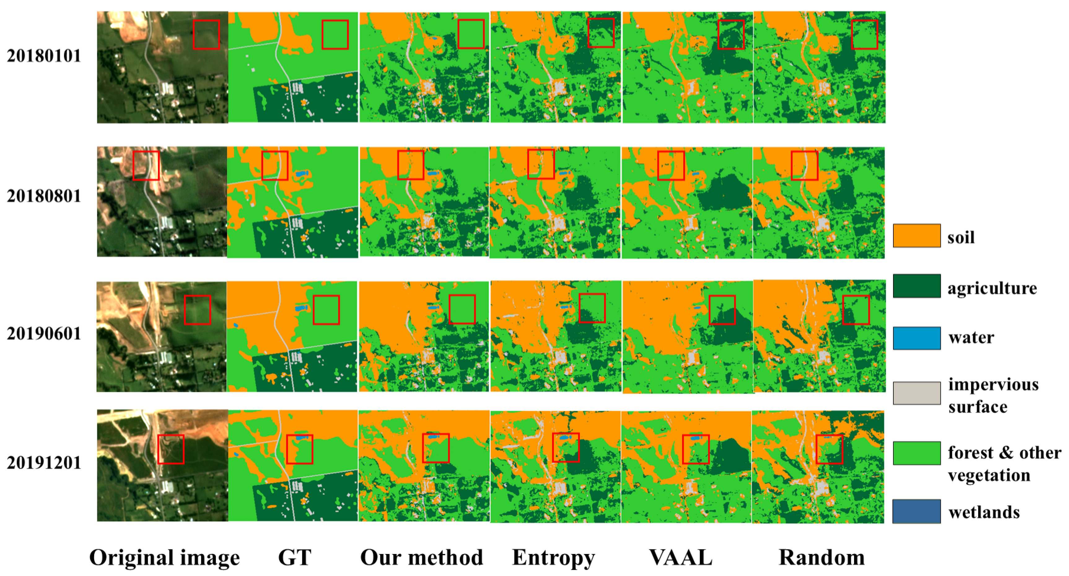
Similar to the scenarios mentioned in the two-class dataset, the reason why the random method is superior to classification entropy is that in the initial stages of training, the temporal classifier has a limited understanding of the distribution of samples. As the number of samples increases, the temporal classifier gains more information. Therefore, entropy sampling can use enough classification information to determine which samples are more informative. This is also why the entropy method gradually gains an advantage. In order to more intuitively understand the effect of classification, we made a comparison between the prediction results of each method and GT when the training set size is 5000, as shown in
Figure 6.
4. Discussion
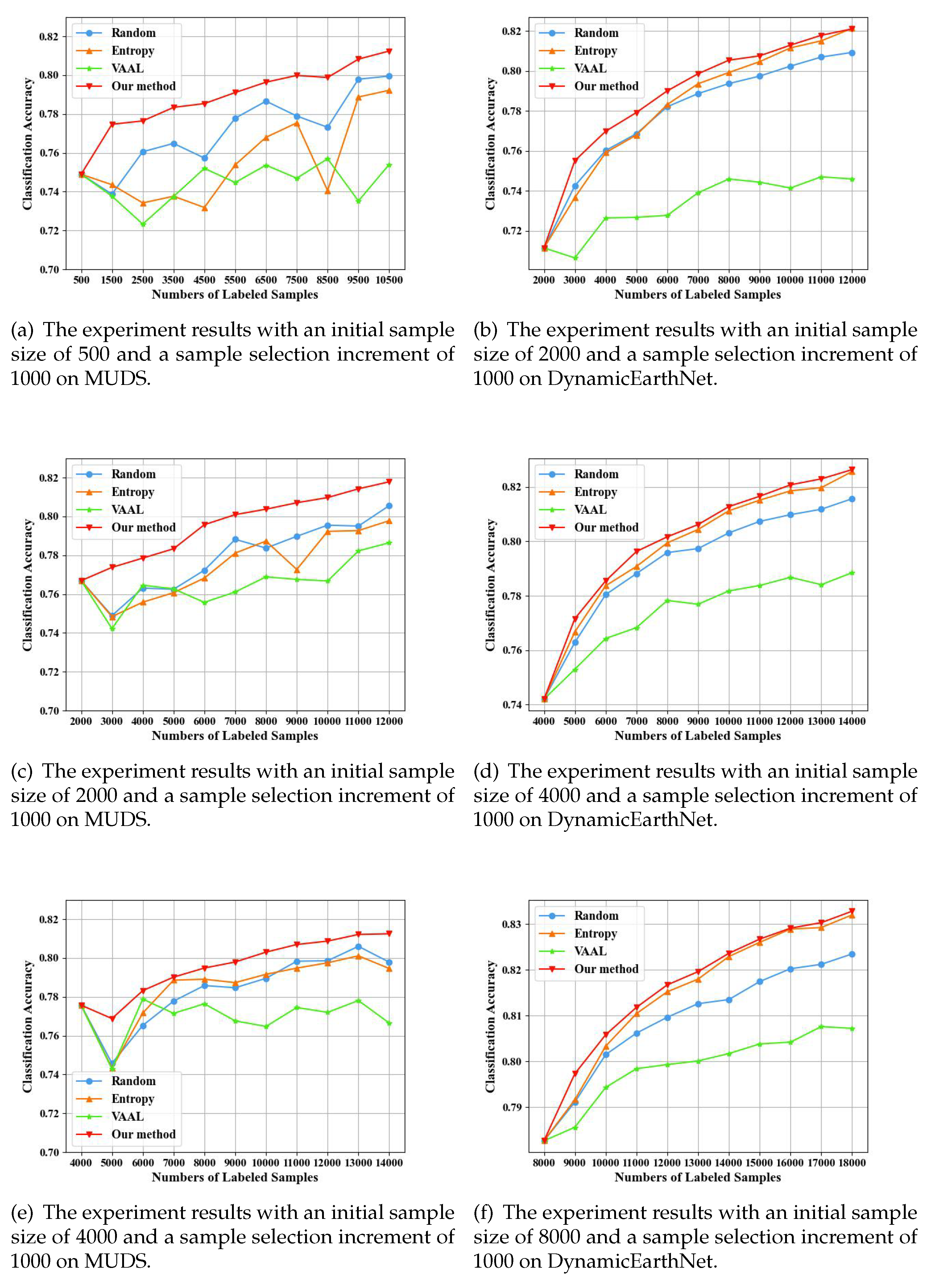
4.1. Experiments with Different Initial Training Sets
Figure 7 illustrates the comparative results of our method under varying initial training set sizes on two datasets. We conducted repeated experiments using different initial training set sizes on the MUDS dataset. It is evident that our method outperforms random sampling, entropy sampling, and VAAL sampling across three different initial training set sizes. Experiments on the Dynamic dataset also indicate the exceptional performance of our method, followed by the entropy sampling. It is evident that our method is effective across different initial training set sizes due to its ability to adapt to varying initial sample quantities and select the most informative data for the classifier from the unlabeled dataset under different initial sample conditions.
4.2. Ablation Study
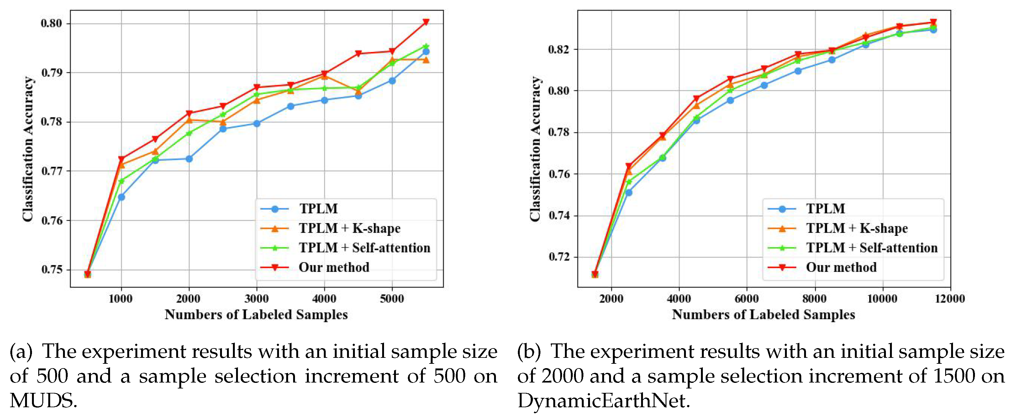
Figure 8 illustrates our ablation study, which was conducted to investigate the contributions of the key modules, K-Shape, and self-attention, in our model. We conducted experiments on two datasets. Specifically, for the MUDS dataset, we set the initial training set sample count to 500 and selected a selection stride of 500. Similarly, for the DynamicEarthNet dataset, the initial training set sample count was set to 2000, with a selection stride of 1500. We performed four sets of experiments: (1)TLPM, (2)TLPM + K-shape, (3)TLPM + self-attention, and (4) our method (TLPM + self-attention + K-shape). Group (1) exhibited the lowest performance among the comparative methods. Group (3) outperformed Group (1), indicating that the standalone TLPM did not focus on the temporal characteristics of the time series samples when predicting loss, whereas the inclusion of self-attention enhanced the model’s predictive loss capability. Group (2) also showed good performance compared to Group (1) due to the consideration of sample distribution properties by the K-Shape method. Notably, the model that incorporated both K-shape and self-attention demonstrated the highest performance, showcasing a significant advantage resulting from the simultaneous consideration of representativeness and uncertainty.
5. Conclusions
This paper presents a new active learning approach for time series classification tasks on remote sensing image datasets. In this approach, we integrate representativeness and uncertainty by employing a K-shape and a time-series loss prediction module equipped with a self-attention mechanism to assess the label value of unlabeled time-series samples. We select the most informative samples to augment the training set and then improve the accuracy of the temporal classifier. We evaluate our proposed method on both a two-class and a multi-class dataset. Experimental results demonstrate its outstanding performance on time series data. Experiments with different initial training sets indicate that our method is effective across different initial training set sizes. Furthermore, ablation experiments were conducted, and the results confirmed the effectiveness of the key modules, K-shape, and self-attention.
Author Contributions
Conceptualization, P.L.; methodology, P.L. and G.X.; software, G.X.; validation, G.X.; data curation, Z.C.,L.C.,Y.M.,L.Z; writing—original draft preparation, G.X. and P.L.; All authors have read and agreed to the published version of the manuscript.
Funding
This work was supported by the National Natural Science Foundation of China (No. U2243222, No. 42071413, and No. 41971397 and 61731022) and Project Y3K0010 and Y7I2160
Data Availability Statement
Conflicts of Interest
The authors declare no conflicts of interest.
Abbreviations
The following abbreviations are used in this manuscript:
| AL |
Active learning |
| TLPM |
Time-series loss prediction module |
| LSTM |
Long short-Term memory |
| GAP |
Global average pooling |
| FC |
Fully connected |
| MUDS |
Multi-temporal urban development spacenet dataset |
| DynamicEarthNet |
Daily multi-Spectral satellite dataset |
| VAAL |
Variational adversarial active learning |
| BANet |
Burned areas neural network |
| GT |
Ground truth |
References
- Liu M, Liu P, Zhao L, et al. Fast semantic segmentation for remote sensing images with an improved Short-Term Dense-Connection (STDC) network. International Journal of Digital Earth, 2024, 17(1): 2356122.
- Zhang Y, Liu P, Chen L, et al. A new multi-source remote sensing image sample dataset with high resolution for flood area extraction: GF-FloodNet. International Journal of Digital Earth, 2023, 16(1): 2522-2554.
- Liu P, Wang L, Ranjan R, et al. A survey on active deep learning: from model driven to data driven. ACM Computing Surveys (CSUR), 2022, 54(10s): 1-34.
- Song B, Liu P, Li J, et al. MLFF-GAN: A multilevel feature fusion with GAN for spatiotemporal remote sensing images. IEEE Transactions on Geoscience and Remote Sensing, 2022, 60: 1-16.
- Liu P, Zhang H, Eom K B. Active deep learning for classification of hyperspectral images. IEEE Journal of Selected Topics in Applied Earth Observations and Remote Sensing, 2016, 10(2): 712-724.
- Lei Z, Zeng Y, Liu P, et al. Active deep learning for hyperspectral image classification with uncertainty learning. IEEE geoscience and remote sensing letters, 2021, 19: 1-5.
- Bortiew A, Patra S, Bruzzone L. Active learning for hyperspectral image classification using kernel sparse representation classifiers. IEEE Geoscience and Remote Sensing Letters, 2023, 20: 1-5.
- Hou W, Chen N, Peng J, et al. A Prototype and Active Learning Network for Small-Sample Hyperspectral Image Classification. IEEE Geoscience and Remote Sensing Letters, 2023.
- Peng F, Luo Q, Ni L M. ACTS: an active learning method for time series classification. IEEE 33rd International Conference on Data Engineering (ICDE). IEEE, 2017: 175-178.
- Pinto M M, Libonati R, Trigo R M, et al. A deep learning approach for mapping and dating burned areas using temporal sequences of satellite images. ISPRS Journal of Photogrammetry and Remote Sensing, 2020, 160: 260-274.
- Sinha S, Ebrahimi S, Darrell T. Variational adversarial active learning. Proceedings of the IEEE/CVF international conference on computer vision. 2019: 5972-5981.
- Paparrizos J, Gravano L. k-shape: Efficient and accurate clustering of time series. Proceedings of the 2015 ACM SIGMOD international conference on management of data. 2015: 1855-1870.
- Yoo D, Kweon I S. Learning loss for active learning. Proceedings of the IEEE/CVF conference on computer vision and pattern recognition. 2019: 93-102.
- M.Lin,Q.Chen, and S. Yan. Network in network. arXiv:1312.4400. [Online]. 2013. Available: http://arxiv.org/abs/1312.4400. arXiv:abs/1312.4400.
- Vaswani, A. Attention is all you need. Advances in Neural Information Processing Systems, 2017.
- Toker A, Kondmann L, Weber M, et al. Dynamicearthnet: Daily multi-spectral satellite dataset for semantic change segmentation. Proceedings of the IEEE/CVF Conference on Computer Vision and Pattern Recognition. 2022: 21158-21167.
- Van Etten A, Hogan D, Manso J M, et al. The multi-temporal urban development spacenet dataset. Proceedings of the IEEE/CVF Conference on Computer Vision and Pattern Recognition. 2021: 6398-6407.
|
Disclaimer/Publisher’s Note: The statements, opinions and data contained in all publications are solely those of the individual author(s) and contributor(s) and not of MDPI and/or the editor(s). MDPI and/or the editor(s) disclaim responsibility for any injury to people or property resulting from any ideas, methods, instructions or products referred to in the content. |
© 2024 by the authors. Licensee MDPI, Basel, Switzerland. This article is an open access article distributed under the terms and conditions of the Creative Commons Attribution (CC BY) license (http://creativecommons.org/licenses/by/4.0/).
