1. Introduction
Identifying unusual structures in images is a challenging problem in computer vision with numerous applications, including industrial inspection [
1,
2], healthcare monitoring [
3,
4], autonomous driving [
5,
6], and video surveillance [
7,
8]. Due to the rarity of encountering defects and the complexity of determining the full specification of defect variations, most literature addresses the Anomaly Detection (AD) problem in unsupervised settings, where a model is only trained on anomaly-free images. However, obtaining training data is expensive and time-consuming, and privacy concerns limit availability, especially in industrial and medical scenarios. Recently computer vision systems have expanded greatly as large-scale datasets, such as ImageNet, have led to a shift from model-driven to data-driven approaches [
9]. For example, in AD, many current state-of-the-art methods rely on deep feature extractors pre-trained on a proxy task on large-scale datasets. In addition to the technical challenges and high costs associated with acquiring and labelling these large datasets, questions have arisen over privacy, ownership, inappropriate content, and unfair biases. This has resulted in ImageNet being restricted to non-commercial applications, the 80M Tiny Images dataset [
10] being withdrawn, promising datasets such as JFT-300M [
11] or Instagram-3.5B [
12] being unavailable for public use, and LAION-5B [
13], which was used to train the famous Stable Diffusion [
14], being withdrawn due to ethical concerns.
“What if we had a way to harness the power of large image datasets with few or none of the major issues and concerns currently faced? [15]".
Fractals are complex geometric structures generated by mathematical equations, thus, anyone can produce the images making them open-source, bypassing massive manual labelling and ethical or bias concerns. The work of Kataoka
et al. [
9] was the first to introduce the possibility of using fractals as an alternative pre-trining method for image recognition tasks. In light of the promising results shown in image classification [
15,
16,
17] and 3D scene understanding [
18], in this paper, we conducted extensive experiments to examine the potential utility of using a synthetically generated dataset composed of fractals for the detection and localization of anomalies such as those representing defects in industrial production processes. We generated two- and three-dimensional fractals following the implementation in [
15,
17] to create standard classification datasets. Moreover, inspired by the semantic segmentation task based on formula-driven supervised learning [
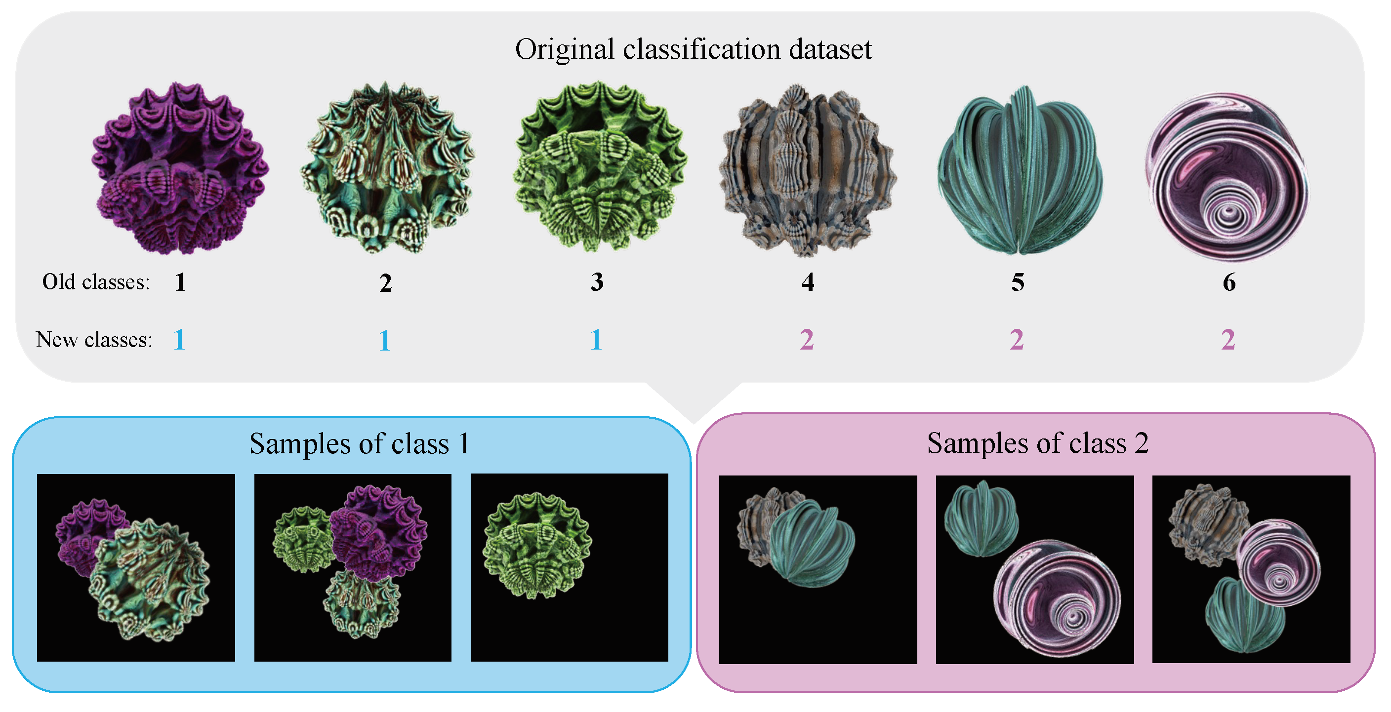
19], we propose a novel approach to combine multiple fractal images. This approach uses groups of fractals to represent different characteristics of each class. A sample of a given class may include a variable number of fractals, which results in a “Multi-Formula” classification dataset (see Figure 3). This introduces more complexity to the classification task with the model being able to learn more discriminative features. Nevertheless, contrary to the existing literature that mainly focuses on fractals’ transfer-learning ability for supervised classification, we compared the AD methods pre-trained with fractals against ImageNet without fine-tuning.
Our contributions are summarised as follows:
We conducted the first systematic analysis comparing the performance of eleven AD models pre-trained with fractals against those pre-trained with ImageNet on three benchmark datasets specifically designed for real-world industrial inspection scenarios, demonstrating that synthetically generated abstract images could be a valid alternative for defect detection.
We analyze the influence of feature hierarchy and object categories in addressing the anomaly detection (AD) task, demonstrating that the effectiveness of fractal-based features is closely tied to the type of anomaly. Nevertheless, we found that low-level fractal features performed better than high-level ones.
We introduce a novel procedure for the generation of classification datasets dubbed “Multi-Formula” that integrates multiple fractals, increasing the number of characteristics for each class and show that this strategy leads to improved performance compared to the standard classification (“Single-Formula”) dataset under the same training condition.
We demonstrate that the learned weights are influenced by the specific fractals used during pre-training, showing that the presence of filters with complex patterns in the early network layers does not necessarily reflect well-learned weights across the entire architecture. On the contrary, higher-level weights may still be poorly optimized. Thus, we emphasize the importance of conducting a comprehensive analysis of the latent space structure to accurately assess the quality of the learned weights.
We evaluated the performance variations when training a model using different dataset configurations, such as fractal structure types, the number of samples, and training settings. Additionally, we observed that careful tuning of model selection is crucial, and reducing the number of samples and classes led to improved anomaly detection performance.
2. Related Works
2.1. Formula-Driven Supervised Learning
Formula-driven supervised learning (FDSL) has recently gained interest in the research community in the context of visual representation learning without real images. By exploiting mathematical formulas and rendering software, FDSL allows the automatic construction of large-scale synthetic datasets, preventing the need for manual labeling and producing a nearly limitless range of images. In this context, several FDSL datasets have been proposed to pre-train computer vision models [
15,
17,
20,
21]. FractalDB [
9] is one of the first datasets presented for image recognition tasks. It consists of colour or grayscale 2D fractal images obtained through an iterated affine function system. The dataset has proven to be effective for CNNs [
9] and ViTs [
16] showing that the pre-trained models tend to focus exclusively on contours to solve the classification task. This discovery leads [
21] to further study the impact of contours in determining the efficacy of the learning of ViTs by proposing ExFractalDB and Radial Contour DataBase (RCDB). The former is composed of grayscale images obtained as projections of 3D fractals. The latter consists of grayscale images of 2D contours and enables a better pertaining than ImageNet-21k when fine-tuned on ImageNet-1k. RCDB pre-training performance on ViTs was outperformed by VisualAtom [
20], a dataset of grayscale images of 2D contours with a larger design space. Yamada
et al. [
18] proposed a point cloud fractal database PC-FractalDB, for 3D object detection. The more recent work of [
17] has surpassed the previously mentioned studies on the classification task by proposing MandelbulbVAR-1k and MandelbulbVAR-Hybrid-21k, two datasets based on a 3D variant of fractals called Mandelbulb which are projected to RGB images.
2.2. Anomaly Detection
The majority of unsupervised AD models fall into two main categories: reconstruction-based and feature embedding-based. This paper focuses on the latter since most state-of-the-art AD methods are feature embedding-based. These methods rely on learning the distribution of anomaly-free data by extracting descriptors from a pre-trained backbone (feature extractor), which is typically kept frozen during the entire AD process. Anomalies are detected during inference as deviations from these anomaly-free features, assuming that the feature extractor produces different features for anomalous images. According to [
22], feature embedding-based methods can be divided into four categories: teacher-student ([
23,
24,
25,
26]), memory bank ([
27,
28,
29]), normalizing flow ([
30,
31]), and one-class classification ([
32,
33]). For teacher-student models, during the training phase, the teacher is the feature extractor and distils the knowledge to the student model. When an abnormal image is passed, the teacher will produce features that the student wasn’t trained on, so the student network won’t be able to replicate the features. Thus, the feature difference in the teacher-student network is the fundamental principle in detecting anomalies during inference. Regarding memory bank-based approaches, features of normal images are extracted from a pre-trained network and stored in a memory bank. Test samples are classified as anomalous if the distance between the extracted test feature and the closest neighbourhood feature point inside the memory bank exceeds a certain threshold. Normalizing flow is used to learn transformations between data distributions. In AD, anomaly-free features are extracted from a pre-trained network and projected by the trainable flow model to an isotropic Gaussian distribution, in other words, the model applies a change of variable formula to fit an arbitrary density to a tractable base distribution. During inference, the normalizing flow is used to estimate the precise likelihood of a test image. Anomalous images should be out of distribution and have a lower likelihood than normal images. For one-class classification, the goal is to identify instances belonging to a single class, without explicitly defining the boundaries between classes as in traditional binary classification.
3. Dataset Generation Methods
3.1. Fractals Images
Fractal images are generated using an Iterated Function System (IFS), composed of two or more functions (called
systems or
codes), each associated with a sampling probability. Affine IFS involves affine transformations:
, where
A represents a linear function and
b represents a translation vector. The set of functions has an associated set of points with a particular geometric structure called
attractor. Following the definition of [
15] and [
9], an IFS system
S, with cardinality
, defined on a complete metric space
is a set of transformations
and their associated probabilities
:
which satisfy the average contractility condition
where
is the Lipschitz constant for
. The attractor
is a unique geometric structure, a subset of
defined by
. The shape of
depends on the function
, while the sampling probabilities
influence the distribution of points on the attractor that are visited during iterations. Affine transform parameters are associated with the categories of the synthetic dataset.
Anderson, and Farrell [
15] improved the sampling strategy to always guarantee the contractility condition of
S and produce fractals with “good” geometric properties. Fractal images with good geometry are not too sparse, containing complex and varied structures with few empty spaces. The linear operator
A of the affine transform must have singular values less than 1 to be a contraction, which can be imposed by construction. Thus, the authors used singular values decomposition of
, where
U and
V are orthogonal matrices and
is a diagonal matrix containing the singular values
and
. By sampling
and
in the range (0, 1), we ensure the system is a contraction. If we consider
and
being rotation matrices of angles
and
and
D a diagonal matrix with diagonal elements
, then
. In this way, we can obtain different
A by sampling
. The translation vector instead, is sampled with
. Regarding good geometry, the authors empirically demonstrate that singular values’ magnitudes dictate how quickly an affine contraction map converges to its fixed point. Small values cause quick collapse, while values near 1 lead to “wandering” trajectories which don’t converge to a clear geometric structure. They empirically find that given
and
as the singular values for
, the
ith function in the system, the majority of the systems with good geometry satisfy
with
being
For , the found range works well, although it may also work for a wider range. Through this paper, this dataset will be called Fractals.
Figure 1.
Examples of samples we generated from a class of Fractals. Note that in [
9] fractals belonging to the same class share similar geometric properties, as they are sampled by slightly perturbing on one of the parameters of the linear operator
A. Contrary in [
15] different fractals are grouped under the same class lacking geometric continuity within samples from the same class.
3.2. Mandelbulb Variations
To generate their dataset, [
17] uses Mandelbulb, an extension to the 3D space of the 2D Mandelbrot, a particular set of fractals. Since fractals are objects with smaller portions similar to larger ones, they can represent infinite levels of smaller detail, and the ability to display them is limited only by computational constraints. This motivated the authors to mostly focus on the rendering part by modelling a parametrized 3D mathematical object, augmenting it by randomly generating colour patterns and shading through a simulated external light source to enhance as many details as possible. Following the formulation in [
17], given
and the following function
:
where
a 3D Mandelbulb is defined as the set of data points
for which the sequence
does not diverge
i.e. when starting from
. In this formulation, the only parameter is
n while for Fractals the set of parameters are:
.
To increase the diversity of generated data by increasing the number of parameters the authors used the Mandelbulb Variant
[
34] based on a new function
parametrized by a vector
equivalent to a boolean vector of length 9. The obtained dataset
MandelbulbVAR-1k is composed of 1037 variations. For more details see [
17,
34]. To overcome the limited number of variants the authors use the Hybrid Mandelbulb Variations, obtained by combining two Mandelbulb Variantions. With this hybrid version, they obtained a dataset with 21k variations,
MandelbulbVAR-Hybrid-21k. Throughout the paper, we will refer to the two datasets collectively as
Mandelbulbs, using specific names when we need to precisely identify one of the two.
Figure 2.
Examples of samples we generated from a class of MandelbulbVAR-1k. We can observe that a class is composed of the same Mandelbulb taken from different perspectives and with various colour patterns ensuring geometric continuity between objects of the same class.
Figure 2.
Examples of samples we generated from a class of MandelbulbVAR-1k. We can observe that a class is composed of the same Mandelbulb taken from different perspectives and with various colour patterns ensuring geometric continuity between objects of the same class.
3.3. Multi-Formula Dataset
We took inspiration from [
15,
19] which use FDSL respectively for semantic segmentation and multi-instance classification. The two approaches create an abstract scene with several different geometric structures within the same image. We adapted the idea of objects of different classes in the same scene to characteristics of the same class in the same image. For example, to classify a house, we may have images of various homes, but what defines a home? For instance, having walls, windows, doors, and a roof are individual characteristics or features that together define a home. We applied the same concepts to fractals. Consider an original dataset composed of
n classes, where each class
(for
) consists of images with a single fractal representing that class. We rearranged the classes to create a new dataset with
m classes, where each new class
(for
) is composed of fractals from multiple classes
. Each sample in this new dataset contains
fractals from class
.
Formally, let the original dataset be where is an image containing a fractal obtained from the mathematical equation , and is its corresponding class label. We construct a new dataset where is an image containing k fractals randomly rescaled and inserted to the image at a random location, and is the new class label. Thus, for each new class , we have . In other words, each class can be considered as a combination of different attributes that could or could not be present. By composing multiple fractals into a single image, we generate multi-formula samples. This is because each class is formed by multiple mathematical formulas that produce distinct fractals. This approach contrasts with the previous datasets, Fractals and Mandelbulbs, where each class was generated by the iteration of a single formula, obtaining single-formula samples. Through the paper, the “Multi-Formula” datasets will be called MultiFractals or MultiMandelbulbs when using respectively Fractals or Mandelbulbs as the source dataset.
Figure 3.
Overview of the proposed “Multi-Formula” dataset. Fractals from different classes from the source dataset are grouped to be the features of new classes, where a variable number of fractals are present in a sample of a class.
Figure 3.
Overview of the proposed “Multi-Formula” dataset. Fractals from different classes from the source dataset are grouped to be the features of new classes, where a variable number of fractals are present in a sample of a class.
4. Implementation Details
The Fractals dataset consists of single-fractal RGB images without background with image resolution
, obtained by grouping 100k IFS codes into 1000 classes. The IFS codes are uniformly sampled for
. We also employ the parameter augmentation method which randomly selects one of the affine transforms (
,
) in the system and scales it by a factor
to get (
,
). We used the official code
1 of [
15] for training since the authors did not release their pre-trained weights. Chiche et al. [
17] released the code
2 for the dataset generation, which we used to create MandelbulbVAR-1k and MandelbulbVAR-Hybrid-21k. However, they did not provide their training code for the anomaly detection task. Therefore, we used the pre-trained weights of WideResNet50 that the authors made available for the analysis of performance with different AD methods.
For the ablation analysis in sec:ablationfdsl, we implemented our training function where for the Mandelbulbs dataset the images of size are randomly cropped to size , following the original implementation. We created MultiFractals and MultiMandelbulbs with 1000 classes using respectively Fractals and MandelbulbVAR-Hybrid-21k as origin datasets. All the mentioned datasets have around 1M samples. We also created a smaller version of the datasets with 200 classes and 400k samples using Fractals and MandelbulbVAR-1k as the source datasets. For a fair comparison, except for Mandelbulbs, all the ablation datasets have images with size . We trained the models with the standard cross-entropy objective function for 100 epochs, with batch sizes of 512 for Fractals and 512 and 1024 for the ablation study, using stochastic gradient descent (SGD) with a momentum value of 0.9, learning rate of 0.1 and weight decay of 1e-4. The images were normalized to the range .
4.1. Datasets:
To investigate what are the performances on the industrial anomaly detection task, our experiments are performed on the MVTecAD [
1], VisA [
35] and MVTec LOCO AD [
2]. MVTecAD contains 15 sub-datasets of industrially manufactured objects. For each object class, the test sets contain both normal and abnormal samples with various defect types. The dataset has a relatively small scale, specifically, the number of training images for each sub-dataset varies from 60 to 391, posing a unique challenge for learning deep representations. VisA contains 12 sub-datasets. The objects range from different types of printed circuit boards to samples with multiple or single instances in a view. MVTec LOCO AD contains 3644 images from five different categories inspired by real-world industrial inspection scenarios with representative samples for structural anomalies such as scratches, dents, or contaminations and logical anomalies like violations of logical constraints, for example, permissible objects occurring in invalid locations.
4.2. Anomaly Detection Methods:
For assessing the anomaly detection performance on MVTecAD and VisA we used the teacher-student methods RD [
24], STFPM [
23], the memory-based methods PatchCore [
27], PaDiM [
28], the flow models FastFlow [
31], C-Flow [
30] and the one-class classification methods PANDA [
32], and CutPaste [
33]. To facilitate reproducibility, we used Anomalib
3 [
36] to train all the methods, except for PANDA
4 [
32] and CutPaste
5 [
33], as well as all the methods used for MVTec LOCO AD, deployed through the official code implementations. For MVTec LOCO AD we used the state-of-the-art methods EfficientAD
6 [
37], PUAD
7 [
38] and SINBAU
8 [
39]. All AD methods use WideResNet50, except for CutPaste, which is implemented with ResNet18.
4.3. Evaluation Metrics:
Image-level metrics are used to assess AD algorithms’ classification performance, whereas pixel-level metrics are used to assess their localization performance. These two types of metrics represent distinct capabilities of AD algorithms, and they are both extremely important. Following prior work we use the area under the receiver operator curve (AUROC) for both image-level and pixel-level anomaly detection. To measure localization performance we also use the area under the per-region-overlap (AUPRO). A significant difference between the PRO score and the ROC measure is that the PRO score weights ground-truth regions of different sizes equally so that it better accommodates varying anomaly sizes, see [
25] for details. For MVTec LOCO AD we also used the saturated per-region overlap (sPRO) introduced in [
2]. It is a generalisation of the PRO metric that takes into account a saturation threshold
s to have a more fair performance evaluation in the case of logical anomalies. Similar to PRO, sPRO does not take into account the false positive rate (FPR). Hence, unless specified the PRO and sPRO values are associated with a FPR of 0.3.
Figure 4.
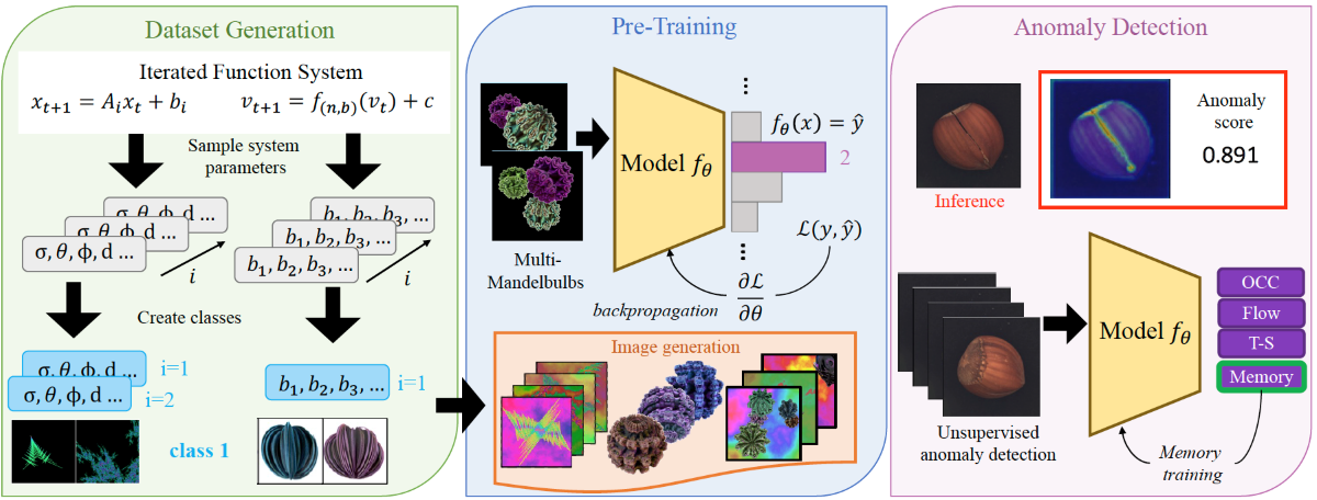
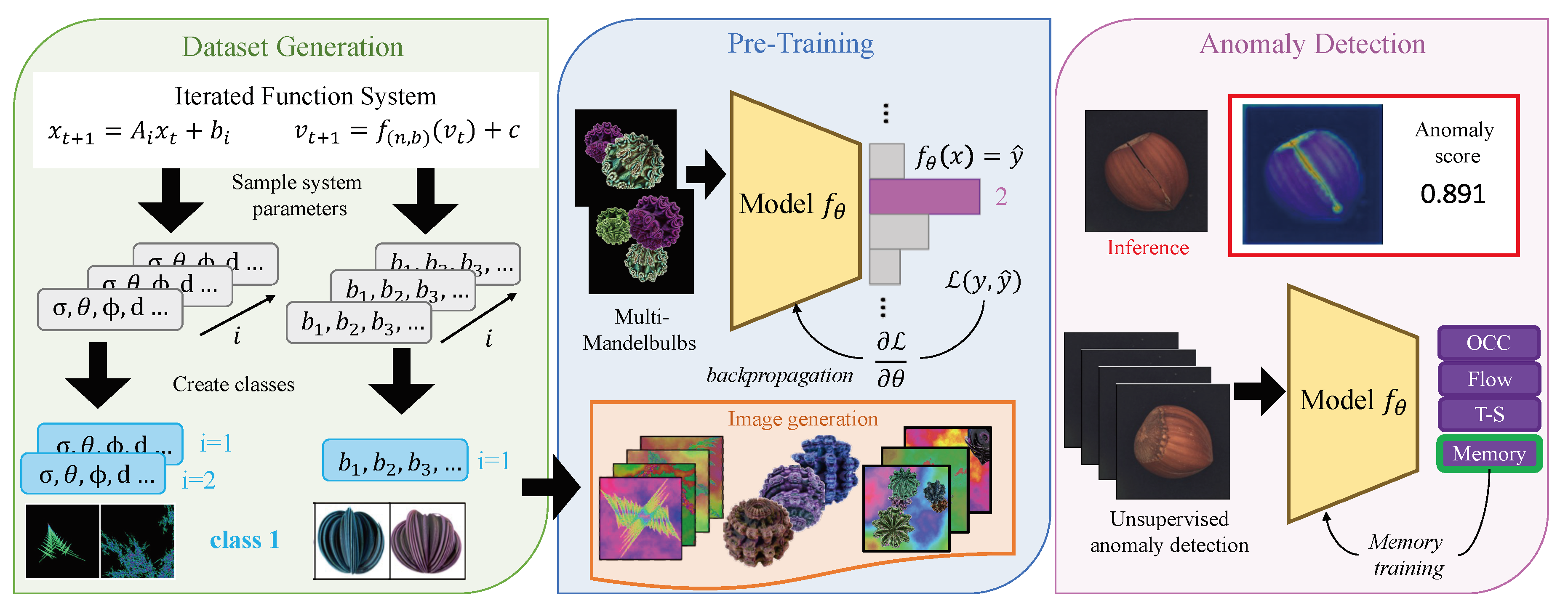
We generate a dataset of IFS codes by sampling the parameters of the system which are used to generate fractals images. A computer vision model for multi-class classification is trained from the generated images, either with a single sample or multiple samples per image. Finally, the model is used as a feature extractor for unsupervised anomaly detection.
5. Performance of Different Anomaly Detection Methods on Fractals Dataset
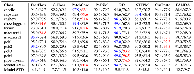
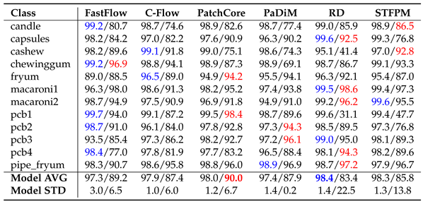
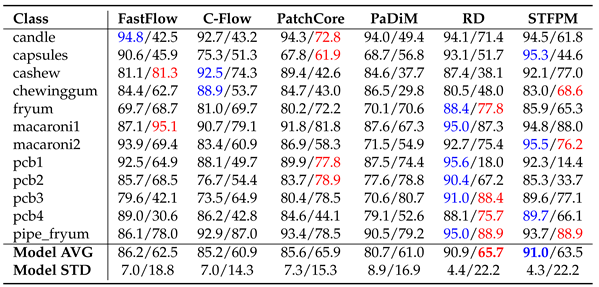
In this section, we analyze the experimental results on MVTecAD and VisA in depth when using Fractals as the pre-training dataset. Note that, except for CutPaste, none of the algorithms had their model weights fine-tuned. In each table the reported metrics are expressed in percentage, the best result for each method is marked in blue for ImageNet and red for Fractals pre-training; in addition, each cell contains the results for ImageNet/Fractals. All the results were obtained with version 0.* of Anomalib.
For MVTecAD the corresponding result are in
Table 1,
Table 2 and
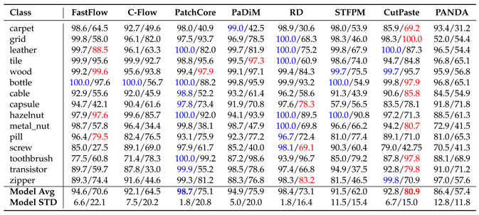
Table 3. In Table 1 we observe that PatchCore is the winning approach followed by RD when using ImageNet as they both solve 7 of the 15 sub-datasets. When using Fractals, CutPaste solves 7 of the 15 classes achieving the highest average image-level AUROC of 80.9%. For some classes Fractals surpass the performance of ImageNet:
grid when using CutPaste and PANDA,
wood with FastFlow and
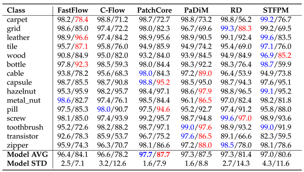
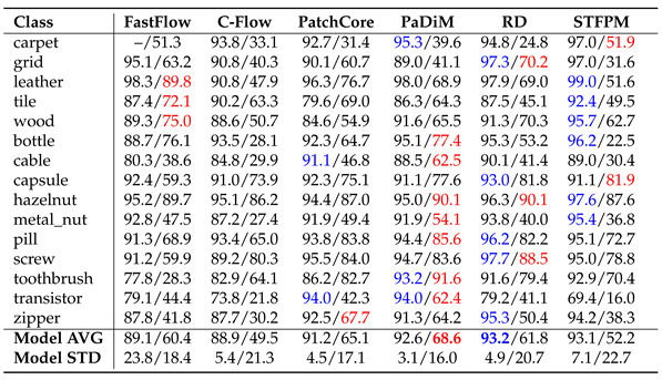
toothbrush with C-Flow, PaDiM, RD and CutPaste. In Table 2 we can see that PatchCore reaches the highest pixel-level AUROC for both ImageNet and Fractals, followed by PaDiM. When using the AUPRO, Fractals’ performance drops. As shown in Table 3, C-Flow is the method that has the biggest drop in localization performance when compared with the results in Table 2. PaDiM reaches the highest AUPRO of 68.9%. Note that the AUPRO metric with the
carpet class for the FastFlow pre-trained with ImageNet is missing. Anomalib [
36], the repository used for the evaluation, led to the invalid score of 1.21, thus, we did not report any value. For VisA the corresponding result Tables are
Table 4,
Table 5 and
Table 6. As shown in Table 4 when using Fractals, PatchCore reached the best score of 80.4% followed by CutPaste with 79.2%. We have some cases where Fractals surpass ImageNet results:
capsules with PatchCore and PANDA,
macaroni2 with CutPaste and PANDA,
pcb1 with PaDiM and CutPaste, and for
pcb2 with PatchCore, PaDiM and CutPaste. Table 5 shows the pixel-level AUROC. For ImageNet the best approach is RD while for Fractals it is PatchCore. On average the pixel-level performance differs around 11% between ImageNet and Fractals. Here, too, using the AUPRO metric results in a performance drop as shown in Table 6.
Overall for both datasets is clear that memory-based methods seem to be the more suitable when using Fractals, while flow-based methods are the ones with the lowest performance. CutPaste works well with fractals reaching the first position on MVTecAD and the second on VisA. For ImageNet the best results remain between teacher-student and memory-based methods. With the AUROC metric, using fractal images leads to promising results both at the image and pixel level. The performance drops when using AUPRO, indicating that small defects are not well localized. Meanwhile, ImageNet weights can maintain good performance across all metrics.
5.1. Comparison between Object Categories
For MVTecAD the 15 sub-datasets can be grouped into textures (carpet, grid, leather, tile, wood) and objects (bottle, cable, capsule, hazelnut, metal_nut, pill, screw, toothbrush, transistor, zipper). For VisA the 12 sub-classes are grouped into pcb (pcb1, pcb2, pcb3, pcb4), images with multi-instance in a view multi-in (candle, capsules, macaroni1, macaroni2) and image with single-instance in a view single-in (cashew, chewinggum, fryum, pipe_fryum). In Figure 5 we can see a qualitative visualization of the image-level AUROC accuracy group by object categories. Focusing on MVTecAD ImageNet leads to good performance for both textures in blue and objects in red for all the methods. The larger blue area shows a higher performance for the texture category. Also with Fractals, we have the same behaviour except for RD and PANDA with objects having respectively +1.9% and +0.7% compared to textures. The bigger difference between textures and objects can be seen for flow-based methods with +7.2% and +6% for FastFlow and C-Flow. With VisA, all methods underperform, for both ImageNet and Fractals, for the multi-in category. Our intuition is that this behaviour is more method-related rather than weight-related. The proposed methods are specialised to perform well on MVTecAD which is composed of images with single objects in a view. For ImageNet pcb and sinle-in have comparable performance, while for Fractals the results are quite variable.
Figure 5.
Spider chart representing average image-level AUROC grouping MVTecAD and VisA classes into different object categories.
Figure 5.
Spider chart representing average image-level AUROC grouping MVTecAD and VisA classes into different object categories.
5.2. Impact of Feature Hierarchy
Feature maps from ResNet-like architectures, which play an important role, can be divided into hierarchy-level
. For example, using the last level for feature representation introduces two problems: (i) the loss of more localized information, as the last layers of the network extract more high-level features, (ii) and the feature bias towards the task of natural image classification which has only little overlap with industrial anomaly detection [
27]. As pointed out by [
9] and [
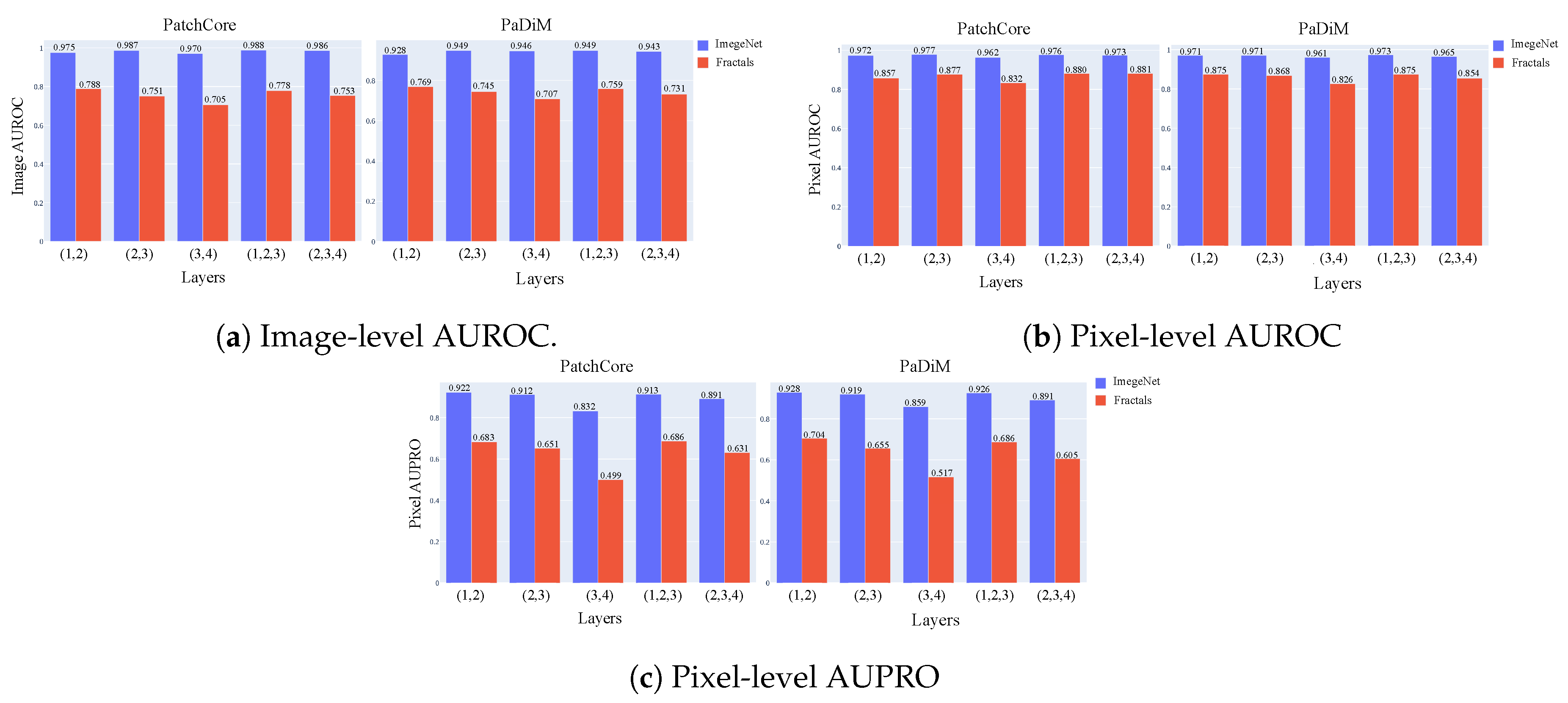
15], models pre-trained on fractal images are unbiased when compared to ImageNet, so we studied the impact of features hierarchy when using Fractals. Figure 6 shows the average image- and pixel-level scores in MVTecAD for PatchCore and PaDiM which rely on
and
for feature representation. For the image-level AUROC when focusing on ImageNet (blue), the results with different hierarchies are quite stable for both methods. Nevertheless, there is not a huge boost in performance when combining three hierarchies instead of two for both ImageNet and Fractals. This outcome is significant as memory-based methods necessitate a large amount of memory during initialization, which increases with the number of features involved. For the pixel-level AUROC, both ImageNet and Fractals show a clear performance drop with
. When using Fractals the best results are obtained with
for PatchCore as well as
and
for PaDiM. We can see that the difference between the results using ImageNet and the results using Fractals is relatively small. This difference increases when considering the AUPRO metrics. When using layers
with Fractals we reach an accuracy of 49.9% for PatchCore and 51.7% for PaDiM.
For Fractals is clear that the best performance is obtained when using low-level features
with a huge drop in performance when involving only high-level features. This could be related to the fact that fractal structures cover more real-world patterns than ImageNet [
18] and low-level features can capture these simpler patterns that can be found in nature. Moreover, FDSL dataset lacks semantic content and as a result, they are potentially not good for semantic-related representation learning [
17] which could be still useful for the AD task.
Figure 6.
Comparison between ImageNet and Fractals pre-training when using different feature hierarchies.
Figure 6.
Comparison between ImageNet and Fractals pre-training when using different feature hierarchies.
6. Performance of Different Anomaly Detection Methods on MandelbulbVAR-1k Dataset
The results presented for MVTecAD (
Table 7,
Table 8 and
Table 9) and VisA (
Table 10,
Table 11 and
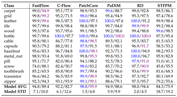
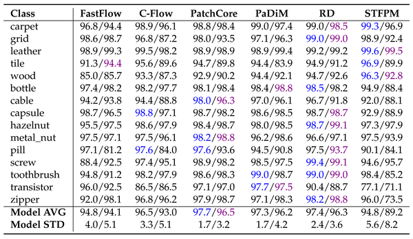
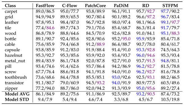
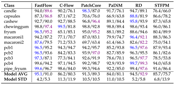
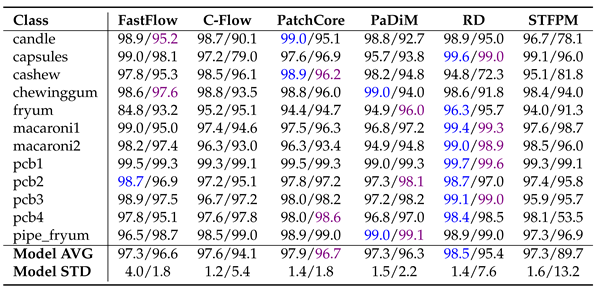
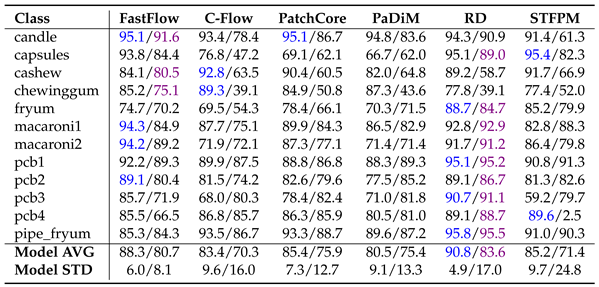
Table 12.) demonstrate that pre-training on MandelbulbVAR-1k achieves performance comparable to ImageNet. In all tables, the metrics are reported as percentages, with the best results for each method highlighted in blue for ImageNet and purple for MandelbulbVAR-1k pre-training; in addition, each cell contains the results for ImageNet/MandelbulbVAR-1k. All the results were obtained with version 1.0 of Anomalib.
From the tables, it is interesting to notice that while flow-based methods, such as FastFlow and Cflow, experienced the largest performance drop when pre-trained on Fractals, they maintained high scores at both the image and pixel levels when using MandelbulbVAR-1k as the pre-training dataset. AUPRO, the metric most negatively impacted by Fractals pre-training, remains close to ImageNet-level performance when using MandelbulbVAR-1k. STFPM exhibits the highest average model standard deviation, making it the least stable method overall. In particular, in Table 12 for the class pcb4, STFPM yields a notably low AUPRO score of 2.5%, raising uncertainty about whether this is an actual result or a potential bug in the library. In general, the leading methods in this evaluation are PatchCore and RD, while STFPM shows highly variable results.
We investigated the impact of feature hierarchy on performance using MandelbulbVAR-1k. In Figure 7, we present the average pixel-level AUROC and AUPRO scores for ImageNet, Fractals, and MandelbulbVAR-1k with PaDiM. The results show that similarly to Fractals, MandelbulbVAR-1k experiences a performance drop when high-level features are used. However, for low- and mid-level hierarchies, MandelbulbVAR-1k achieves performance very close to ImageNet. When analyzing higher-level hierarchies (i.e., and ), both Fractals and MandelbulbVAR-1k exhibit a consistent decline in performance. Interestingly, for the AUPRO metric, MandelbulbVAR-1k performs worse than Fractals at higher feature hierarchies, indicating that Mandelbulb pre-training struggles to localize small anomalies precisely when using high-level features.
Overall, it is clear that for FDSL the model trained with MandelbulbVAR-1k outperforms Fractals. However, ImageNet remains the best pre-training dataset, particularly due to its stable performance across different feature hierarchies. Nevertheless, MandelbulbVAR-1k produces results that are very close to ImageNet, which is promising, since abstract images have a significantly different distribution from natural images used for anomaly detection.
Figure 7.
Comparison between ImageNet, Fractals and MandelbulbVAR-1k pre-training when using different feature hierarchies on PaDiM.
Figure 7.
Comparison between ImageNet, Fractals and MandelbulbVAR-1k pre-training when using different feature hierarchies on PaDiM.
6.1. Visualization of Learned Low-Level Filters
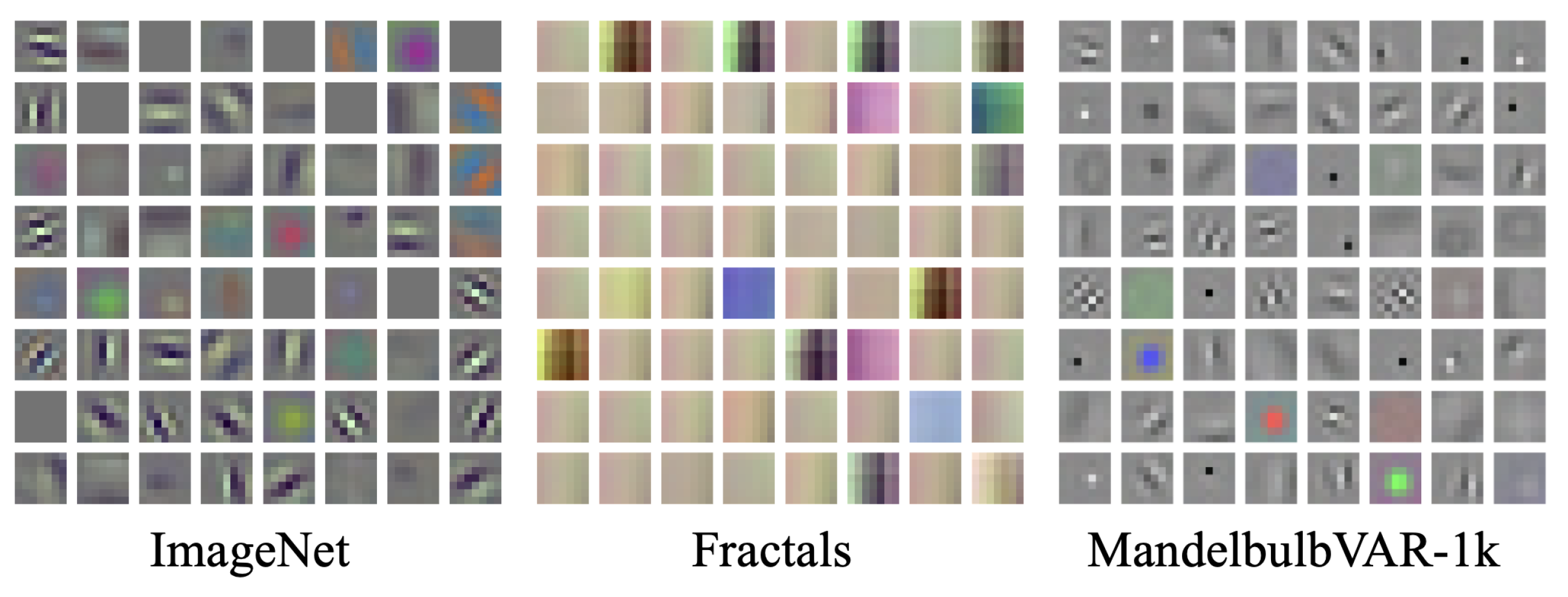
Figure 8 shows the filters from the first layer of WideResNet-50 backbones that give the results reported in the previous sections. We can see that the weights learned using Fractals show simple patterns, such as solid vertical or horizontal lines. This means that the model has learned more basic features in the input data. When using MandelbulbVAR-1k, some filters exhibit similarities to those in ImageNet, such as Gabor-like and coloured Gaussian-like filters, along with similar grey-toned backgrounds. This suggests that MandelbulbVAR-1k can capture complex structures in the data, much like ImageNet, enabling the extraction of more intricate features.
Figure 8.
Comparison of the filters from the first convolutional layer of WideResNet50 pre-trained with different datasets.
Figure 8.
Comparison of the filters from the first convolutional layer of WideResNet50 pre-trained with different datasets.
6.2. Qualitative Results
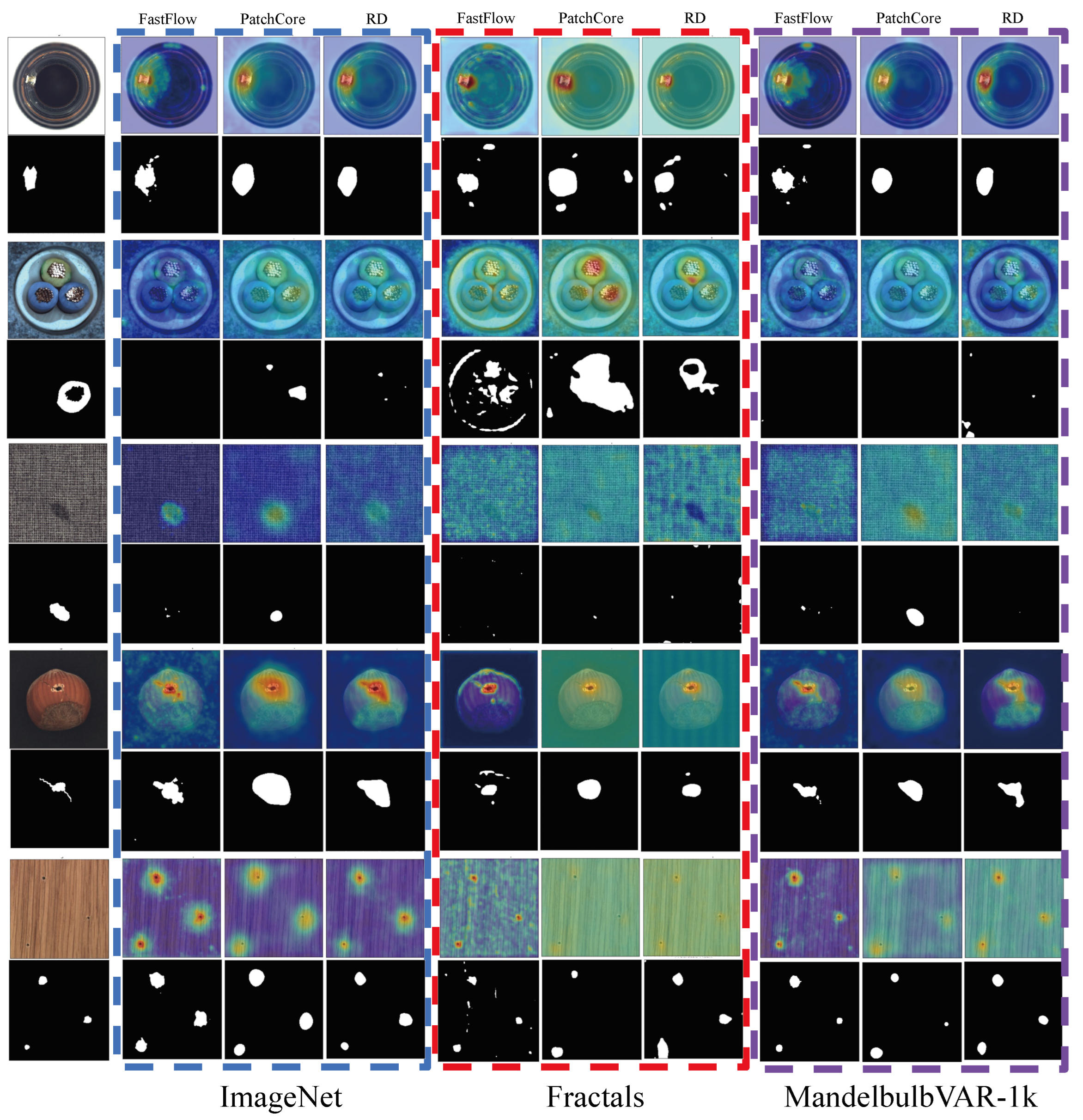
In Figure 9 we can see some qualitative results on MVTecAD’s classes: bottle, cable, carpet, hazelnut and wood. In the coloured boxes, we have the predicted heat maps and segmentation mask for ImageNet, Fractals and MandelbulbVAR-1k. It is interesting to notice that for cable the anomaly type is called cable_swap so rather than a structural defect such as scratches, dents, colour spots or cracks, we are facing a misplacement, a violation of the position of an object which can be seen as a logical anomaly like the one finds in MVTec LOCO AD. We can see from the figure that, with none of the pre-training datasets, the AD methods can predict the correct segmentation mask. We also observe that Fractals tend to struggle with localizing anomalies that have low contrast with the background, such as in the carpet class. In contrast, when using PatchCore with ImageNet or MandelbulbVAR-1k, we can successfully localize the colour stain. From a qualitative perspective, we observe that using MandelbulbVAR-1k produces predictions that closely resemble those from ImageNet. In certain cases, such as the hazelnut class or for carpet with PatchCore, MandelbulbVAR-1k generates more refined and accurate segmentation masks.
Figure 9.
Qualitative visualization for the MVTecAD’s classes: bottle, cable, carpet, hazelnut and wood. In the first column, we have the original image and the ground-truth. In the blue box we have the anomaly score and predicted segmentation mask for ImageNet pre-training, in the red box for Fractals and the purple box for MandelbulbVAR-1k.
7. Ablation Study
In the FDSL scenario, based on the results of the
Section 5 and
Section 6, we can conclude that PatchCore using MandelbulbVAR-1k offers the best solution, achieving results that closely match those of ImageNet pre-training. This section explores key dataset characteristics in depth by comparing various generated datasets. Since Chiche
et al. [
17] did not provide an official training function, we performed the ablation using our code. We used PatchCore’s official code
9 for the experiments, utilizing the default configuration, and conducted evaluations on the MVTec AD dataset. We stopped the training once the model achieved 100% validation accuracy, as the classification task was fully resolved and continuing training would no longer provide any benefit. The average results for the different pre-trained datasets are reported in Table 13 where for each dataset the number of classes is reported in brackets. As mentioned in sec:implemetationdetails, when using 1000 classes (1000 cl.) the training samples are around 1M, when using 200 classes (200 cl.) they are 400k. As a convenience, we will refer to the dataset with 200 classes as “-small” from now on.
For a fair comparison and to establish a baseline reference, we trained the model with Mandelbulb VAR-1k, referred to as “Mandelbulbs” for simplicity. This distinction helps differentiate the results obtained from our custom training functions versus those using the official pre-trained weights. Unexpectedly Mandelbulbs lead to worse performances than a randomly initialised network. The surprisingly good results from the random network are closely linked to PatchCore’s memory-based strategy. Normality is determined by comparing stored features, so even with random weights, the descriptors remain meaningful for anomaly detection since the process relies on distinguishing between stored and non-stored features. Our pre-training with Mandelbulbs resulted in an image-level AUROC of 67.8% and a pixel-level AUROC of 78.4%, which is significantly lower than the results reported in the original paper [
17] (97.2% and 96.8%, respectively). The multi-formula strategy substantially boosts performance, with MultiMandelbulbs achieving +13.1% and +13.5% compared to Mandelbulbs in terms of image and pixel level AUROC. MultiMandelbulbs-small reached the second-best performance after ImageNet. This result is significant, as it demonstrates that we can achieve better performance with half the samples and only 1/5 of the classes. We investigated whether the performance boost was due to the reduced number of samples and classes or the multi-formula strategy, so we trained the feature extractor with Mandlebulbs-small and the results showed a slight improvement over Mandelbulbs, with a +1.7% increase in image- and +1.8% in pixel-level accuracy. Moreover, when comparing Fractals-small and MultiFractals-small, we observed a performance increase of +5.1% and +7.7% confirming that the performance gains are due to the multi-formula strategy, not the type of abstract figure, or the number of samples used for generating the dataset. We also compare the performance when using a background (see “MultiMandelbulbs-back” on Table 13 and we follow the same background creation of [
15]. Contrary to the background impact in [
15] we obtain a reduction in performance compared to the case without background with both 1000 and 200 classes. Using the best FDSL as baseline (“MultiMandelbulbs (200 cl.)”), we analysed the impact of adding some random transforms (“MultiMandelbulbs-transforms (200 cl.)”) like in [
15], but this led to a slight reduction in performance of -2.6% and -0.9%. Finally, we trained the model using grayscale images (“MultiMandelbulbs-gray (200 cl.)”) to prevent the model from relying on colour patterns to differentiate between classes. This resulted in reduced performance, most likely because the MVTec AD dataset contains coloured images, so some colour information was still required to distinguish defects.
Table 13.
Average image and pixel level AUROC express in % for PatchCore [
27] using WideResNet-50 feature extractor on MVTec AD. The “Pre-training” column indicates which dataset has been used for pre-training, and in brackets indicate the number of classes in each dataset. Best, and second-best scores are shown in underlined bold, and bold, respectively.
| Pre-training |
Image AUROC |
Pixel AUROC |
| Random initialization |
0.772 |
0.860 |
| ImangenNet (1000 cl.) |
0.991 |
0.981 |
| Mandelbulbs (1000 cl.) |
0.678 |
0.784 |
| MultiMandelbulbs (1000 cl.) |
0.809 |
0.919 |
| MultiMandelbulbs-back (1000 cl.) |
0.719 |
0.833 |
| Fractals (200 cl.) |
0.720 |
0.823 |
| MultiFractals (200 cl.) |
0.771 |
0.900 |
| Mandelbulbs (200 cl.) |
0.695 |
0.802 |
| MultiMandlebulbs (200 cl.) |
0.817 |
0.921 |
| MultiMandelbulbs-back (200 cl.) |
0.699 |
0.781 |
| MultiMandelbulbs-transforms (200 cl.) |
0.791 |
0.912 |
| MultiMandelbulbs-gray (200 cl.) |
0.793 |
0.908 |
7.1. Convergence Speed in FDSL Training
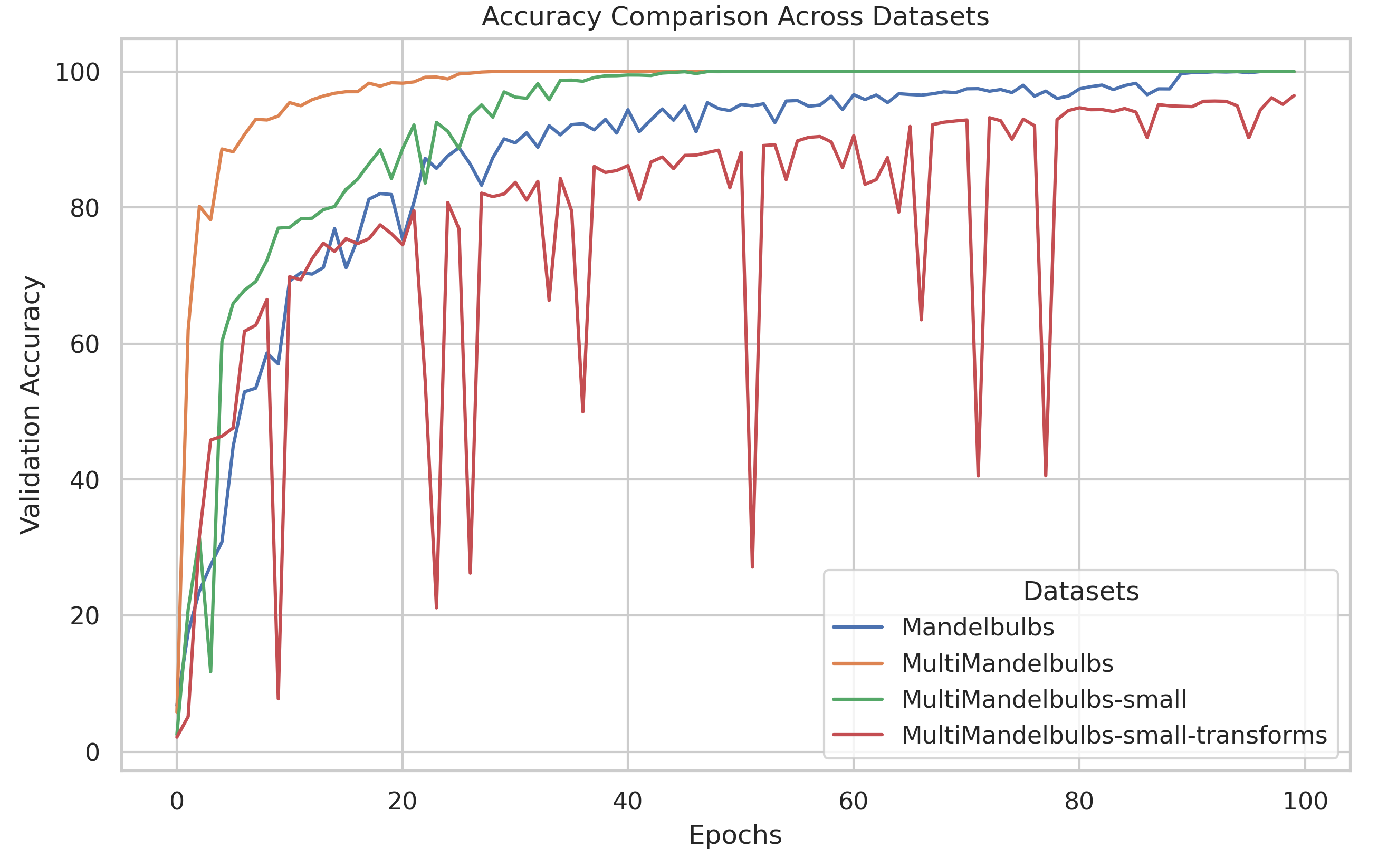
We observed that training speed varies with the dataset. For instance, when using Multi-Formula datasets, the classification task achieved 100% validation accuracy more quickly than with standard datasets. Our deduction is that, since we have a mixture of samples for each image the network is exposed to samples from the same classes more frequently during each epoch. Let’s consider in Figure 3 the sample corresponding to the “Old class” with label 5 (in green) it is present in all the three generated images related to the “New class” with label 2, meaning the network has three chances to see that samples during training. This behaviour likely explains the difference in training speed. For instance, Mandelbulbs achieved 100% validation accuracy only towards the end of a 20-day training period on 4 NVIDIA A100 GPUs with a total batch size of 1024 and 100 epochs. MultiMandelbulbs-small completed 100 epochs in less than 6 days, reaching 100% accuracy between epoch 30 and 40. In our hardware configuration, stopping the training around epoch 30 will reduce the training time to around 2 days. In Figure 10 we observed the validation accuracy across different pre-training datasets, with MultiMandelbulbs showing the fastest convergence. Interestingly, incorporating transformations during training significantly affects both convergence speed and overall performance (as we see in Table 13).
Figure 10.
Top-1 classification accuracy during training for different generated datasets.
Figure 10.
Top-1 classification accuracy during training for different generated datasets.
7.2. Low- and High-Level Features Analysis
Figure 11 shows the filters from the first layer of WideResNet-50 backbones that give the results reported in Table 13. We can see that the learned weights have similar patterns to the original weights shown in Figure 8.
Figure 11.
Comparison of the filters from the first convolutional layer of WideResNet50 pre-trained with different datasets configuration.
Figure 11.
Comparison of the filters from the first convolutional layer of WideResNet50 pre-trained with different datasets configuration.
Filter visualization helps examine the learned weights in the first layers, providing insights into the low-level features extracted by the pre-trained model.
As discussed in sec:featureshierarchy we found that FDSL struggles to learn effective high-level features. This observation aligns with the findings reported in [
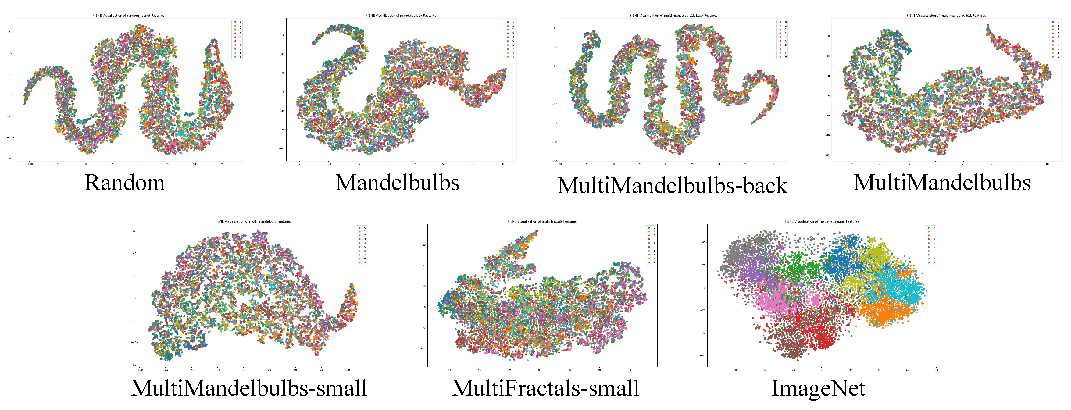
17]. This aspect was further explored by analyzing the t-SNE plot on CIFAR10. In Figure 12 we present the plots for the different pre-trained backbones listed in Table 13 without fine-tuning. The figure shows that pre-training with ImageNet results in a backbone that effectively clusters CIFAR-10 images, even without fine-tuning. This is likely due to ImageNet’s large-scale dataset with diverse classes, which may overlap with the types of objects in CIFAR-10. In the case of random initialization (Random), it is interesting to observe the shape of the plot. ImageNet’s t-SNE plot shows a spherical shape with a more spread-out sample distribution, indicating that the network effectively projects data features evenly across the high-dimensional space. In contrast, the random network exhibits an elongated shape, suggesting that features are concentrated in a specific region of the latent space. Surprisingly, Mandelbulbs also shows a latent space with a similar “sinusoidal” pattern to the random network. This pattern indicates that, in the final layers where semantic understanding happens, Mandelbulbs behaves similarly to a random network. This might suggest either that the data has a dominant direction or trend or that the network struggles to find an effective weight set to evenly distribute points in the latent space. Moreover, no cluster is formed, which is an expected behaviour. This sinusoidal shape is maintained also for MultiMandeblulbs with and without background. With MultiMandelbubls-small and MultiFractals-small we start to see a more spread shape.
These results highlight that relying solely on visualizing the filters of the first convolution layer may lead to the premature conclusion that the learned weights are effective. However, this does not guarantee a comprehensive understanding of the model’s learning process. A thorough analysis of the latent space should be incorporated to gain deeper insights into the network’s representations.
Figure 12.
The t-SNE plot of CIFAR-10 validation set, using WideResNet-50 pre-trained on different datasets, is presented. We extracted feature vectors from the penultimate layers, prior to the final classification layers, without any fine-tuning.
Figure 12.
The t-SNE plot of CIFAR-10 validation set, using WideResNet-50 pre-trained on different datasets, is presented. We extracted feature vectors from the penultimate layers, prior to the final classification layers, without any fine-tuning.
7.3. Impact of Training Configuration
In line with other FDSL implementations, we used the same dataset for both training and validation, as the primary goal is to improve downstream task performance. However, the literature has not thoroughly explored key aspects like optimal training and validation accuracy, the relationship between training-validation splits, data transformations, and how these factors influence model selection, leaving this critical area largely underinvestigated. We opted to follow the code configuration outlined in [
9], also followed by [
17] for training the network in the downstream classification task (not for anomaly detection). The key difference between our implementation and the one in [
9] lies in the data transformations applied during training and validation. In [
9], the training set consists of images sized at
, randomly cropped to
and normalized to a mean of 0.2 and a standard deviation of 0.5. In contrast, the validation set, which is identical to the training set, undergoes resizing to
and is subjected to the same normalization process. The batch size is 512, moreover, a scheduler is applied where the learning rate is divided by 10 at epochs 30 and 60. The rest of the training configuration was kept the same as in the ablation study discussed in sec:ablationfdsl. We want to emphasize that, while the authors claim to have trained MandelbulbVAR-1k for 600 epochs, we trained for only 100 epochs to maintain consistency with the ablation results presented in Table 13.
We evaluated the impact of different training configurations using the MultiMandelbulbs-small dataset, which emerged as the most effective pretraining dataset in our ablation study (Table 13). Three configurations were tested: the first, referred to as “VAR1”, follows the setup described earlier, inspired by [
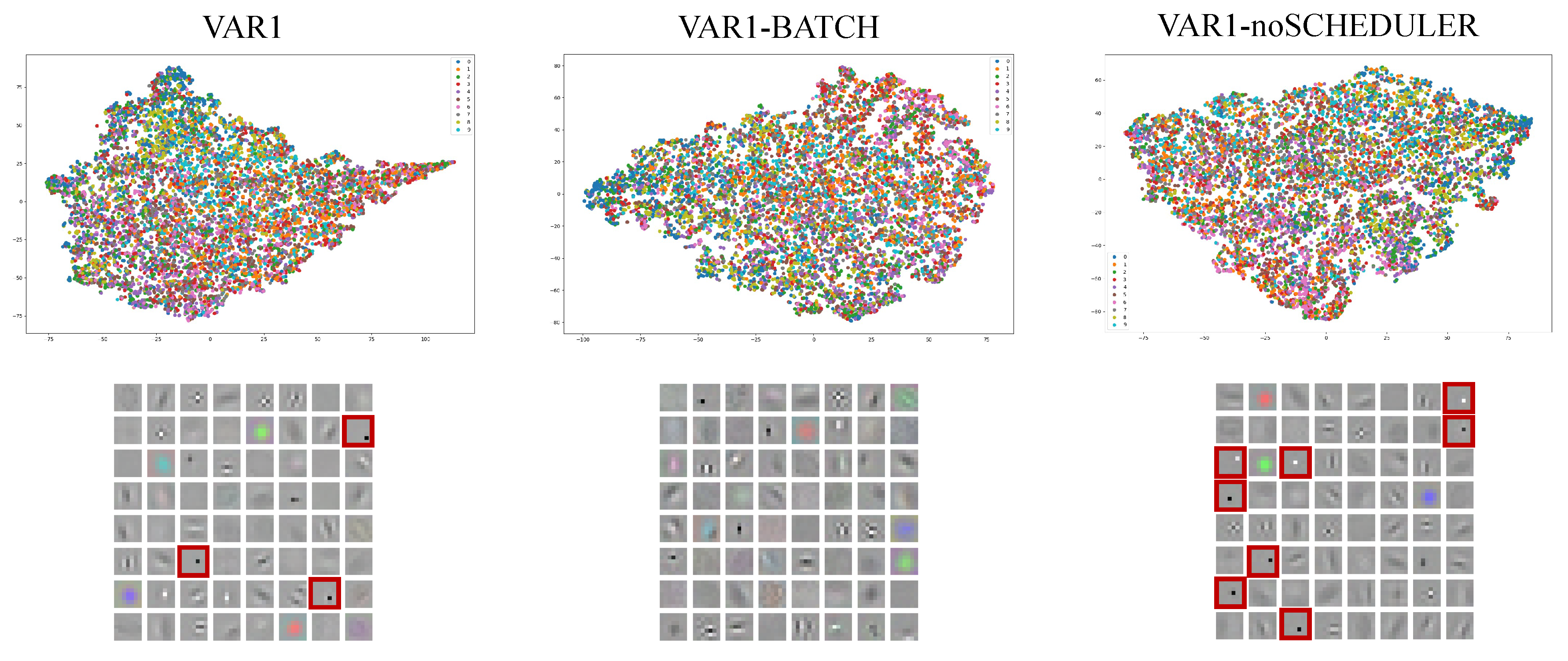
9]. In the second configuration, “VAR1-BATCH”, we increased the batch size from 512 to 1024, matching the original batch size used in the ablation study, while keeping the same scheduler. The third configuration, “VAR1-noSCHEDULER”, retains the batch size of 512 but omits the scheduler, aligning with the setup used in the ablation study. In Figure 13 we reported how the image- and pixel-level AUROC, when using PatchCore as AD method, change at different training epochs. We can see that “VAR1” is the best-performing configuration while “VAR1-BATCH” is the worst one. It’s interesting to observe that AUROC scores are not directly related to validation accuracy, for example, in “VAR1” the highest image-level AUROC is at epoch 40 with a score of 0.865 and a validation accuracy of 4.94%, while the highest pixel-level accuracy is achieved at epoch 80 with a score of 0.942 and validation accuracy of 8.95%. The best model selected during training is epoch 83 with the highest validation accuracy of 9.33% resulting in an image and pixel AUROC of 0.857 and 0.941 (see Table 14). If we observe the image-level AUROC, the one obtained with the highest validation accuracy (0.857) is lower than the one obtained at epoch 40 (0.865). This highlights that with FDSL, clarity in train configuration and model selection is crucial.
Figure 13.
Image- (left) and pixel-level (right) AUROC scores achieved with PatchCore at various epochs of the pre-training stage using different training configurations.
Figure 13.
Image- (left) and pixel-level (right) AUROC scores achieved with PatchCore at various epochs of the pre-training stage using different training configurations.
In Figure 14, we present the t-SNE plot of the CIFAR-10 validation set. It is noteworthy that, compared to the baseline latent space for MultiMandelbulbs-small shown in Figure 8, the latent space structure exhibits an even more spherical organization. This shift in structure highlights the impact of the training configuration on the representation of the data. For example, in “VAR1-noSCHEDULER”, which mirrors our ablation training settings except for the initial transform applied to the training and validation sets and the batch size, we observe significant improvements in the latent space. This structure closely resembles what we achieve using ImageNet. For “VAR1”, the best-performing method in our experiments, we observe a spherical latent space with an elongated region on the right side of the t-SNE plot. This suggests that while “VAR1” performs well for PatchCore, the quality of high-level features in certain areas of the latent space may not be fully optimized.
In Figure 14 we can also see the filters from the first layer of WideResNet-50. The filters of “VAR1-noSCHEDULER” are closer to the filters of MandelbulbVAR-1k (see Figure 8) in particular the “dot-like” pattern.
Table 14.
Results of the best-performing model for each training configuration. The table shows the epoch at which the best model was selected, along with the corresponding validation accuracy and AUROC score achieved using PatchCore.
Table 14.
Results of the best-performing model for each training configuration. The table shows the epoch at which the best model was selected, along with the corresponding validation accuracy and AUROC score achieved using PatchCore.
| Train Config. |
Best Epoch |
Best Val. Acc. |
Image AUROC |
Pixel AUROC |
| VAR1 |
83 |
9.33 |
0.857 |
0.941 |
| VAR1-BATCH |
25 |
10.01 |
0.836 |
0.932 |
| VAR1-noSCHEDULER |
97 |
16.69 |
0.844 |
0.931 |
Figure 14.
Comparison of the filters from the first convolutional layer of WideResNet-50 that give the results reported in Table 14. Some of the “dot-like” filters are framed in red.
Figure 14.
Comparison of the filters from the first convolutional layer of WideResNet-50 that give the results reported in Table 14. Some of the “dot-like” filters are framed in red.
7.4. Results on MVTec LOCO AD
We further investigate the influence of training configuration and the significance of the latent space by comparing pre-training on ImageNet and MultiMandelbulbs-small.
Table 15 and
Table 16 present the results for the MultiMandelbulbs-small dataset, where we compare the original training setup from sec:ablationfdsl (Baseline) with the three variations introduced in sec:trainconfig (VAR1, VAR1-BATCH, VAR1-noSCHEDULER). These configurations are evaluated on the MVTec LOCO AD dataset. Unlike MVTecAD and VisA, MVTec LOCO AD poses a greater challenge as it contains structural and logical anomalies. In particular, addressing logical anomalies requires learned weights that can extract semantic representations which align with learning meaningful high-level features. However, a latent space with an elongated structure may compromise the overall quality of these learned representations. The tables below highlight the best results for the different training configurations for MultiMandelbulbs-small in orange. In Table 15 we have the image-level AUROC for three different AD methods, where all the variations adopted in sec:trainconfig lead to an improvement in performance compared to the “Beseline”. For EfficientAD, the optimal configuration is “VAR1”, achieving a score of 0.811. For PUAD, the best-performing setup is “VAR1-BATCH” with a score of 0.837, while for SINBAD, the top result is obtained with “VAR1-noSCHEDULER”, scoring 0.788. The common factor of the different configurations compared to the “Baseline” is the different set of transforms applied to the training and validation set which follow [
9]. Other training configurations, such as the scheduler and batch size, also affect performance depending on the specific AD model. For instance, in SINBAD, the score increases from 0.734 to 0.788 when the scheduler is removed. This highlights the strong correlation between model selection in FDSL and the AD method used in downstream tasks. In Table 16 we reported the results for EfficientAD using pixel-level sPRO obtained using the official evaluation code
10 of MVTec LOCO AD. The sPRO score provides more precise localization results. The table shows that “VAR1” remains the best-performing configuration for EfficientAD.
8. Conclusions
We chose to focus on industrial visual inspection, a specialized field often constrained by data scarcity due to strict privacy regulations and the high cost of labelling. Defect detection, in particular, requires robust features capable of discerning even minor visual variations as normal and abnormal samples look similar but differ in local appearance. Large-scale datasets like ImageNet are highly valuable for pre-training models in cold-start defect detection. However, large datasets have the potential to violate ethical or privacy standards. In such cases, these datasets may be suspended from functionality, face ownership shifts, or be abruptly withdrawn. Such scenarios can complicate the tracking of lineages, raise concerns regarding privacy and data integrity, and make it difficult to assign credit to data sources. In industrial defect detection with limited access to high-quality labelled data, relying solely on supervised methods becomes increasingly impractical due to the data-hungry nature of deep learning models. Our work diverges from the standard approaches in AD by exploring the use of abstract images as an alternative pre-training. We investigate the impact of pre-training with fractals compared to ImageNet on established AD methods. Unlike conventional FDSL approaches that rely on fractal fine-tuning, we deliberately exclude this step to maintain consistency with the original AD methods, which do not involve fine-tuning (except for CutPaste, which includes fine-tuning by default).
We conducted a systematic analysis of 11 state-of-the-art AD methods and tested their performance on 32 object classes each having different types of anomalies. Experiments reveal that memory-based methods and CutPaste seem statistically better than others and their results vary depending on the type of objects’ class, emphasizing the importance of anomaly type selection when considering fractal images. We observed that low-level fractal features are more effective and an in-depth analysis of the latent space should be considered to understand the quality of the learned weights. We observed that MandelbulbVAR-1k can reach very close results to ImageNet both from the qualitative and quantitative point of view. We introduce a new way of combining the dynamically generated abstract image generating a “Multi-Formula” dataset, showing a high improvement in performance compared to the standard classification datasets under the same training conditions. Additionally, we observed that training configuration and model selection require careful tuning and investigation as it could completely change the quality of the learned weights, particularly the high-level features. Although pre-training with ImageNet remains a clear winner on this task, our findings motivate a new research direction in AD, where there is the potential to replace large-scale natural datasets with completely synthetic abstract datasets reducing annotation labour, protecting fairness, and preserving privacy.
In future works, our studies may be continued in a variety of ways. First, FDSL requires further investigation, especially in developing more advanced pre-training strategies to enhance high-level features. Addressing this gap could bring FDSL closer to the performance levels of ImageNet-based feature extractors, improving off-the-shelf models for cold-start anomaly detection. Second, we observe that in the literature key aspects like optimal training and validation accuracy, the relationship between training-validation splits, data transformations, and how these factors influence model selection have not been thoroughly explored, and we have shown in our study that they highly impact the final performance. Third, our “Multi-Formula” dataset is created by randomly grouping fractal images into new classes. Future investigations should explore the correlation between model performance and how these fractal images are grouped, as well as a deeper analysis of the maximum number of fractals in an image. Additionally, the impact of performance relative to the number of classes should also be examined. Fourth, limited effort has been made to synthesize abnormal samples through data augmentation, a challenging but crucial task. More focus should be given to self-supervised methods like CutPaste, which generate synthetic anomalies. Finally, fractals’ performance under few-shot learning should be investigated. Using fractal pre-trained weights could reduce the amount of data needed for fine-tuning in fields with limited data, like medicine.
Author Contributions
Conceptualization, C.I.U., E.C. and O.L; methodology, C.I.U.; software, C.I.U.; validation, C.I.U.; formal analysis, C.I.U.; investigation, C.I.U.; writing—original draft preparation, C.I.U.; writing—review and editing, C.I.U., E.C. and O.L.; visualization, C.I.U.; funding acquisition, O.L. All authors have read and agreed to the published version of the manuscript.
Funding
The research presented in this paper was funded by
Data Availability Statement
Conflicts of Interest
The authors declare no conflicts of interest.
Abbreviations
The following abbreviations are used in this manuscript:
| AD |
Anomaly Detection |
| FDSL |
Formula-Driven Supervised Learning |
| IFS |
Iterated Function System |
References
- Bergmann, P.; Fauser, M.; Sattlegger, D.; Steger, C. MVTec AD–A comprehensive real-world dataset for unsupervised anomaly detection. Proceedings of the IEEE/CVF conference on computer vision and pattern recognition, 2019, pp. 9592–9600.
- Bergmann, P.; Batzner, K.; Fauser, M.; Sattlegger, D.; Steger, C. Beyond dents and scratches: Logical constraints in unsupervised anomaly detection and localization. International Journal of Computer Vision 2022, 130, 947–969. [Google Scholar] [CrossRef]
- Zimmerer, D.; Full, P.M.; Isensee, F.; Jäger, P.; Adler, T.; Petersen, J.; Köhler, G.; Ross, T.; Reinke, A.; Kascenas, A.; others. Mood 2020: A public benchmark for out-of-distribution detection and localization on medical images. IEEE Transactions on Medical Imaging 2022, 41, 2728–2738. [Google Scholar] [CrossRef] [PubMed]
- Menze, B.H.; Jakab, A.; Bauer, S.; Kalpathy-Cramer, J.; Farahani, K.; Kirby, J.; Burren, Y.; Porz, N.; Slotboom, J.; Wiest, R.; others. The multimodal brain tumor image segmentation benchmark (BRATS). IEEE transactions on medical imaging 2014, 34, 1993–2024. [Google Scholar] [CrossRef] [PubMed]
- Blum, H.; Sarlin, P.E.; Nieto, J.; Siegwart, R.; Cadena, C. Fishyscapes: A benchmark for safe semantic segmentation in autonomous driving. proceedings of the IEEE/CVF international conference on computer vision workshops, 2019, pp. 0–0.
- Hendrycks, D.; Basart, S.; Mazeika, M.; Zou, A.; Kwon, J.; Mostajabi, M.; Steinhardt, J.; Song, D. Scaling out-of-distribution detection for real-world settings. arXiv preprint arXiv:1911.11132 2019.
- Liu, W.; Luo, W.; Lian, D.; Gao, S. Future frame prediction for anomaly detection–a new baseline. Proceedings of the IEEE conference on computer vision and pattern recognition, 2018, pp. 6536–6545.
- Nazare, T.S.; de Mello, R.F.; Ponti, M.A. Are pre-trained CNNs good feature extractors for anomaly detection in surveillance videos? arXiv preprint arXiv:1811.08495 2018.
- Kataoka, H.; Okayasu, K.; Matsumoto, A.; Yamagata, E.; Yamada, R.; Inoue, N.; Nakamura, A.; Satoh, Y. Pre-training without natural images. Proceedings of the Asian Conference on Computer Vision, 2020.
- Torralba, A.; Fergus, R.; Freeman, W.T. 80 million tiny images: A large data set for nonparametric object and scene recognition. IEEE transactions on pattern analysis and machine intelligence 2008, 30, 1958–1970. [Google Scholar] [CrossRef] [PubMed]
- Sun, C.; Shrivastava, A.; Singh, S.; Gupta, A. Revisiting unreasonable effectiveness of data in deep learning era. Proceedings of the IEEE international conference on computer vision, 2017, pp. 843–852.
- Mahajan, D.; Girshick, R.; Ramanathan, V.; He, K.; Paluri, M.; Li, Y.; Bharambe, A.; Van Der Maaten, L. Exploring the limits of weakly supervised pretraining. Proceedings of the European conference on computer vision (ECCV), 2018, pp. 181–196.
- Schuhmann, C.; Beaumont, R.; Vencu, R.; Gordon, C.; Wightman, R.; Cherti, M.; Coombes, T.; Katta, A.; Mullis, C.; Wortsman, M.; others. Laion-5b: An open large-scale dataset for training next generation image-text models. Advances in Neural Information Processing Systems 2022, 35, 25278–25294. [Google Scholar]
- Rombach, R.; Blattmann, A.; Lorenz, D.; Esser, P.; Ommer, B. High-Resolution Image Synthesis with Latent Diffusion Models, 2021, [arXiv:cs.CV/2112.10752].
- Anderson, C.; Farrell, R. Improving fractal pre-training. Proceedings of the IEEE/CVF Winter Conference on Applications of Computer Vision, 2022, pp. 1300–1309.
- Nakashima, K.; Kataoka, H.; Matsumoto, A.; Iwata, K.; Inoue, N.; Satoh, Y. Can vision transformers learn without natural images? Proceedings of the AAAI Conference on Artificial Intelligence, 2022, Vol. 36, pp. 1990–1998.
- Chiche, B.N.; Horikawa, Y.; Fujita, R. Pre-training Vision Models with Mandelbulb Variations. Proceedings of the IEEE/CVF Conference on Computer Vision and Pattern Recognition, 2024, pp. 22062–22071.
- Yamada, R.; Kataoka, H.; Chiba, N.; Domae, Y.; Ogata, T. Point cloud pre-training with natural 3D structures. Proceedings of the IEEE/CVF Conference on Computer Vision and Pattern Recognition, 2022, pp. 21283–21293.
- Shinoda, R.; Hayamizu, R.; Nakashima, K.; Inoue, N.; Yokota, R.; Kataoka, H. Segrcdb: Semantic segmentation via formula-driven supervised learning. Proceedings of the IEEE/CVF International Conference on Computer Vision, 2023, pp. 20054–20063.
- Takashima, S.; Hayamizu, R.; Inoue, N.; Kataoka, H.; Yokota, R. Visual atoms: Pre-training vision transformers with sinusoidal waves. Proceedings of the IEEE/CVF Conference on Computer Vision and Pattern Recognition, 2023, pp. 18579–18588.
- Kataoka, H.; Hayamizu, R.; Yamada, R.; Nakashima, K.; Takashima, S.; Zhang, X.; Martinez-Noriega, E.J.; Inoue, N.; Yokota, R. Replacing labeled real-image datasets with auto-generated contours. Proceedings of the IEEE/CVF Conference on Computer Vision and Pattern Recognition, 2022, pp. 21232–21241.
- Xie, G.; Wang, J.; Liu, J.; Lyu, J.; Liu, Y.; Wang, C.; Zheng, F.; Jin, Y. Im-iad: Industrial image anomaly detection benchmark in manufacturing. arXiv preprint arXiv:2301.13359 2023.
- Wang, G.; Han, S.; Ding, E.; Huang, D. Student-teacher feature pyramid matching for anomaly detection. arXiv preprint arXiv:2103.04257 2021.
- Deng, H.; Li, X. Anomaly detection via reverse distillation from one-class embedding. Proceedings of the IEEE/CVF Conference on Computer Vision and Pattern Recognition, 2022, pp. 9737–9746.
- Bergmann, P.; Fauser, M.; Sattlegger, D.; Steger, C. Uninformed students: Student-teacher anomaly detection with discriminative latent embeddings. Proceedings of the IEEE/CVF conference on computer vision and pattern recognition, 2020, pp. 4183–4192.
- Guo, J.; Lu, S.; Jia, L.; Zhang, W.; Li, H. ReContrast: Domain-Specific Anomaly Detection via Contrastive Reconstruction. arXiv preprint arXiv:2306.02602 2023.
- Roth, K.; Pemula, L.; Zepeda, J.; Schölkopf, B.; Brox, T.; Gehler, P. Towards total recall in industrial anomaly detection. Proceedings of the IEEE/CVF Conference on Computer Vision and Pattern Recognition, 2022, pp. 14318–14328.
- Defard, T.; Setkov, A.; Loesch, A.; Audigier, R. Padim: a patch distribution modeling framework for anomaly detection and localization. International Conference on Pattern Recognition. Springer, 2021, pp. 475–489.
- Lee, S.; Lee, S.; Song, B.C. Cfa: Coupled-hypersphere-based feature adaptation for target-oriented anomaly localization. IEEE Access 2022, 10, 78446–78454. [Google Scholar] [CrossRef]
- Gudovskiy, D.; Ishizaka, S.; Kozuka, K. Cflow-ad: Real-time unsupervised anomaly detection with localization via conditional normalizing flows. Proceedings of the IEEE/CVF Winter Conference on Applications of Computer Vision, 2022, pp. 98–107.
- Yu, J.; Zheng, Y.; Wang, X.; Li, W.; Wu, Y.; Zhao, R.; Wu, L. Fastflow: Unsupervised anomaly detection and localization via 2d normalizing flows. arXiv preprint arXiv:2111.07677 2021.
- Reiss, T.; Cohen, N.; Bergman, L.; Hoshen, Y. Panda: Adapting pretrained features for anomaly detection and segmentation. Proceedings of the IEEE/CVF Conference on Computer Vision and Pattern Recognition, 2021, pp. 2806–2814.
- Li, C.L.; Sohn, K.; Yoon, J.; Pfister, T. Cutpaste: Self-supervised learning for anomaly detection and localization. Proceedings of the IEEE/CVF conference on computer vision and pattern recognition, 2021, pp. 9664–9674.
- Rampe, J. New mandelbulb variations. https://softologyblog.wordpress.com/2011/07/21/, 2011. Accessed: 2024-07-22.
- Zou, Y.; Jeong, J.; Pemula, L.; Zhang, D.; Dabeer, O. Spot-the-difference self-supervised pre-training for anomaly detection and segmentation. European Conference on Computer Vision. Springer, 2022, pp. 392–408.
- Akcay, S.; Ameln, D.; Vaidya, A.; Lakshmanan, B.; Ahuja, N.; Genc, U. Anomalib: A deep learning library for anomaly detection. 2022 IEEE International Conference on Image Processing (ICIP). IEEE, 2022, pp. 1706–1710.
- Batzner, K.; Heckler, L.; König, R. Efficientad: Accurate visual anomaly detection at millisecond-level latencies. Proceedings of the IEEE/CVF Winter Conference on Applications of Computer Vision, 2024, pp. 128–138.
- Sugawara, S.; Imamura, R. PUAD: Frustratingly Simple Method for Robust Anomaly Detection. arXiv preprint arXiv:2402.15143 2024.
- Cohen, N.; Tzachor, I.; Hoshen, Y. Set Features for Anomaly Detection. arXiv preprint arXiv:2311.14773 2023.
|
Disclaimer/Publisher’s Note: The statements, opinions and data contained in all publications are solely those of the individual author(s) and contributor(s) and not of MDPI and/or the editor(s). MDPI and/or the editor(s) disclaim responsibility for any injury to people or property resulting from any ideas, methods, instructions or products referred to in the content. |
© 2024 by the authors. Licensee MDPI, Basel, Switzerland. This article is an open access article distributed under the terms and conditions of the Creative Commons Attribution (CC BY) license (http://creativecommons.org/licenses/by/4.0/).
