Modelling and Analysis of the Transverse Surface Roughness in Hollow Core Fibers

The corrugation of the interfaces of the cross-section of hollow core fibers based on the inhibited coupling waveguiding mechanism is modeled and the impact on propagation loss is analyzed. The proposed model is based on a combined use of coupled mode theory and azimuthal decomposition. It shows that such transverse roughness causes coupling between the core modes and the dielectric modes of the cladding and consequently an increase of the fiber loss. The model is validated by comparing theoretical and numerical results obtained by applying both deterministic and stochastic corrugations to tube lattice and nested fibers. Scaling laws and impact of fiber parameters are discussed. The model shows that the loss increase is not directly correlated to the root mean square of the stochastic roughness, but only to the value of the power spectral density in specific spatial frequency ranges.

Keywords:

Subject:

Engineering - Telecommunications

1. Introduction

In the last fifteen years, Hollow-Core Photonic Crystal Fibers based on the Inhibited Coupling guidance mechanism (IC-HCPCF) have experienced an impressive loss reduction up to and recently overtaking the Rayleigh scattering limit on a wide range of wavelengths, spanning from UV and visible [1] to near infrared [2,3]. At first, researchers’ efforts were focused on Confinement Loss (CL) reduction. CL is the only loss mechanism in ideal IC-HCPCFs. It is caused by the combined effects of residual coupling with cladding modes and tunneling through the microstructured cladding [4]. The introduction of the negative curvature core-cladding interface [5], together with the proposal first [6] and fabrication soon after [7] of Tube Lattice Fibers (TLF), followed by the conceptualization and fabrication of nested [8], node-less [9], conjoint tubes [10], and hybrid cladding [11] fibers, pushed CL down by several orders of magnitude.

Gradually, the research effort moved toward other loss mechanisms caused by imperfect manufacturing processes and thus not occurring in ideal fibers. Currently, the two main mechanisms identified by the research community are Microbending Loss (MBL) and Surface Scattering Loss (SSL). MBL is a stochastic phenomenon consisting in microscopic and random deflections of the fiber axis from the ideal straight longitudinal direction. The axis deflection introduces a coupling of the Fundamental Core Mode (FCM) with other modes, causing a power drainage which increases the propagation loss [12,13]. SSL originates from the fact that the interfaces of the microstructured cladding are not completely flat, as assumed in ideal fibers, but exhibit a random corrugation. This roughness is generated by frozen-in thermal surface capillary waves (SCW) caused by the interplay between thermal noise and glass interface surface tension as the fiber is drawn [14,15]. Due to its thermodynamic cause, surface roughness cannot be completely eliminated. However, recently a new drawing technique based on counter-directional gas and dielectric flows during fiber drawing has been proposed and implemented, showing a significant reduction of surface roughness [1]. So far, all the modeling based both on rigorous [13] and heuristic approaches [9,12] focused on the effect of surface roughness along the propagation direction, usually identified with the z-axis (z-roughness). On the surfaces there is also a transverse roughness (t-roughness), related to the stochastic corrugation on the transverse plane and affecting the fiber cross-section. Unlike z-roughness, t-roughness has been until now scarcely investigated [16,17]. In this context, in the this work we present a theoretical model of the t-roughness and an analysis of its impact on TLF-like IC-HCPCF loss. The approach is based on the combined use of Coupled Mode Theory (CMT) and Azimuthal Fourier Decomposition (AFD) [18,19]. The model shows that t-roughness induces an additional coupling between FCM and Dielectric Modes (DMs), that is those modes which are mainly confined in the cladding membranes. The coupling causes a power drainage from FCM to DMs with a loss increase caused to the former. The model also shows that only a specific range of the Power Spectral Density (PSD) of the stochastic process describing the roughness is involved in the loss increase. A technique for numerically studying stochastic t-roughness is also introduced. The model is finally validated and the t-roughness impact is quantified, by considering both TLFs and nested fibers.

2. Modeling

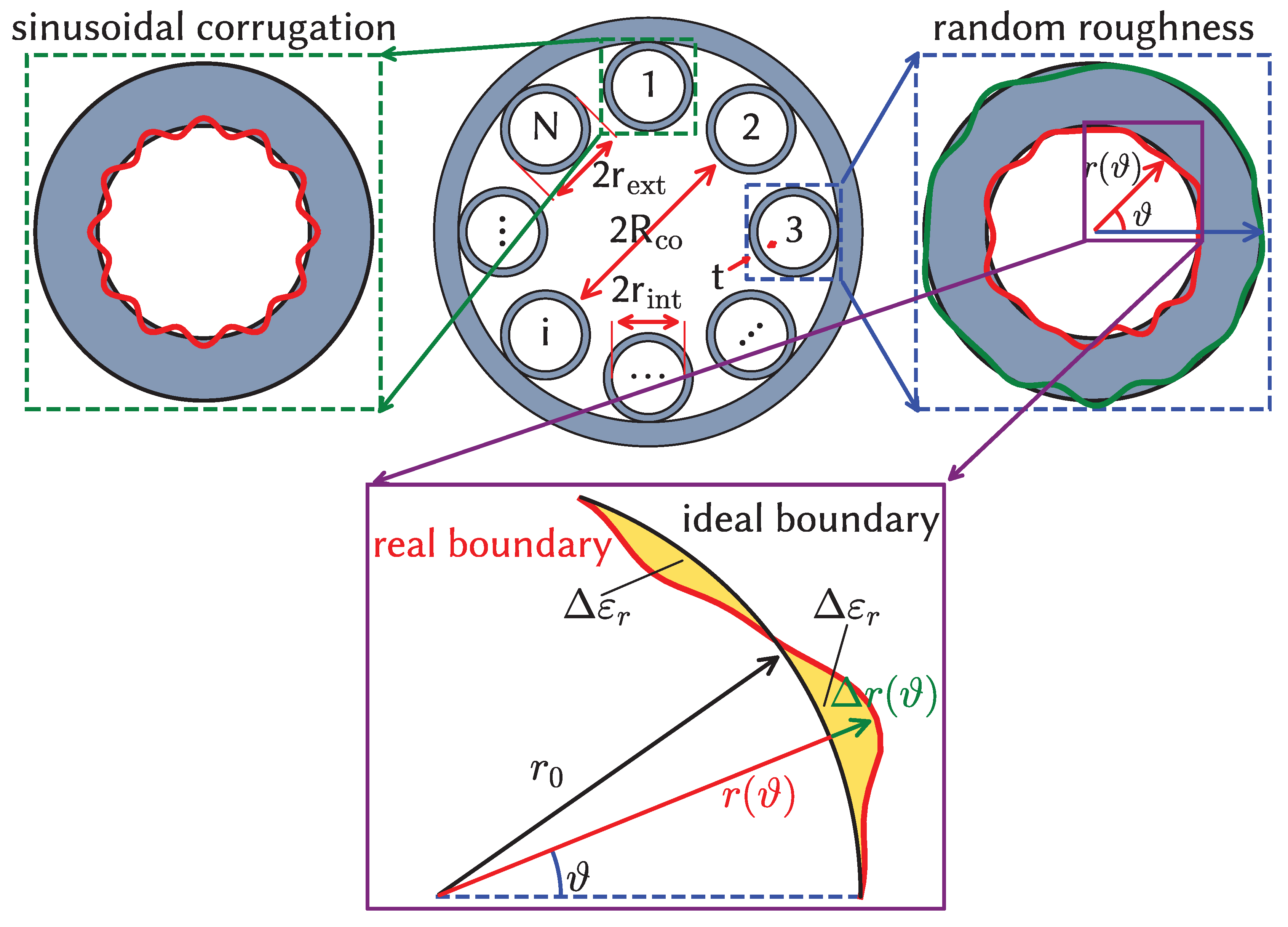
For the sake of analysis, let us consider a Tube Lattice Fiber (TLF). The basic cross section and the geometrical parameters are shown in Figure 1. This kind of IC-HCPCF consists in an arrangement of

N_{t}

elements separating the hollow-core from the homogeneous external jacket, with the goal to decouple as much as possible the light confined in the core from the continuum of radiating waves in the jacket.

Let us assume that the tube interfaces are affected by a deformation due to roughness on the transverse plane, as shown in the right inset of Figure 1. In the context of single tube approximation [20], and by assuming the roughness in each tube is uncorrelated with that in the other ones, each tube can be analyzed separately. By introducing a local polar frame of reference

(r, θ)

centered at the center of the tube and shown in Figure 1, the deformation is described by a displacement

Δ r (θ)

of the real surface outlined by the function

r (θ)

with respect to the perfectly circular ideal one with radius

r_{0} = r_{i n t}, r_{e x t}

for the inner and outer surface, respectively. In the context of CMT, this can be modeled in terms of a dielectric permittivity perturbation:

Δ ϵ = ϵ_{r}^{r e a l} - ϵ_{r}^{i d e a l}

(1)

where

ϵ_{r}^{r e a l}

is the function describing the permittivity of the real fiber and

ϵ_{r}^{i d e a l}

is that of the ideal one. The perturbation can cause coupling among the fiber modes. Even though the approach is completely general, here, for the sake of simplicity, we focus on the effects of FCM coupling to DMs [4,20].

DMs feature two different polarizations, called

E H

and

H E

, and are described by two indices

μ

and

ν

E H

and

H E

polarizations have the dominant electric field component aligned along the radial and azimuthal direction, respectively. The azimuthal index

μ

corresponds to the number of periods that the dominant electric field component shows along the azimuthal direction, and the radial index

ν

is the total number of maxima and minima of the dominant electric field component along the radial direction.

2.1. Coupling Coefficient Calculation

Let us consider the coupling between the FCM and the DM having indices

μ

and

ν

. The DM polarization can be either

E H

H E

. The coupling coefficient is:

k = \frac{π}{2 η_{0}} \frac{1}{λ} {\int \int}_{S_{d}} Δ ϵ_{r} {\bar{E}}_{F C M} \cdot {\bar{E}}_{D M}^{*} d S,

(2)

where

η_{0}

is the free space impedance,

λ

is the wavelength,

{\bar{E}}_{F C M}

and

{\bar{E}}_{D M}

are the power-normalized electric field transverse components of the FCM and CLM of the ideal fiber, respectively, and

S_{d}

is the region of the fiber cross section where

Δ ϵ_{r} \neq 0

. On each of the two interfaces, the perturbation can be written as:

Δ ϵ_{r} = - q \{\begin{matrix} (1 - n_{d}^{2}); if r_{0} < r (θ) < r_{0} + Δ r (θ) and Δ r \geq 0 \\ (n_{d}^{2} - 1); if r_{0} + Δ r (θ) < r (θ) < r_{0} and Δ r < 0 \end{matrix}

with

q = \{\begin{matrix} - 1 if r_{0} = r_{e x t} \\ 1 if r_{0} = r_{i n t} \end{matrix}

We assume

Δ r < < t, λ

, and

r_{0}

; in that case, the core and cladding mode field distributions can be assumed to be almost constant between

r_{0}

and

r_{0} + Δ r

{\bar{E}}_{F C M} (r, θ) ≃ {\bar{E}}_{F C M} (r_{0}, θ)

{\bar{E}}_{D M} (r, θ) ≃ {\bar{E}}_{D M} (r_{0}, θ)

, and Equation (2) can be approximated as:

k ≃ \frac{q π}{2 η_{0}} \frac{n_{d}^{2} - 1}{r_{0} λ} \int_{0}^{2 π} {\bar{E}}_{F C M} (r_{0}, θ) \cdot {\bar{E}}_{D M}^{*} (r_{0}, θ) Δ r (θ) d θ .

(3)

In order to analyze how the value of the integral in Equation (3), and thus the coupling strength, depends on the FCM and DM field distributions, the Azimuthal Fourier Decomposition (AFD) [18] can be applied to the radial and azimuthal components

E_{F C M}^{r}

and

E_{F C M}^{θ}

of the FCM and to the perturbation

Δ r (θ)

E_{F C M}^{s} (r_{0}, θ) = \sum_{m_{=} - \infty}^{+ \infty} R_{m}^{s} e^{- j m θ},

(4)

Δ r (θ) = \sum_{m = - \infty}^{+ \infty} C_{m} e^{- j m θ},

(5)

with

s = r, θ

. The sets

{R_{m}^{s}}

and

{C_{m}}

contain the Azimuthal Fourier Spectra (AFS) of the FCM electric field components and of the perturbation calculated on the circle of radius

r_{0}

. They represent the amplitude of the spatial harmonics at spatial frequency

\tilde{f} = m / (2 π r_{0})

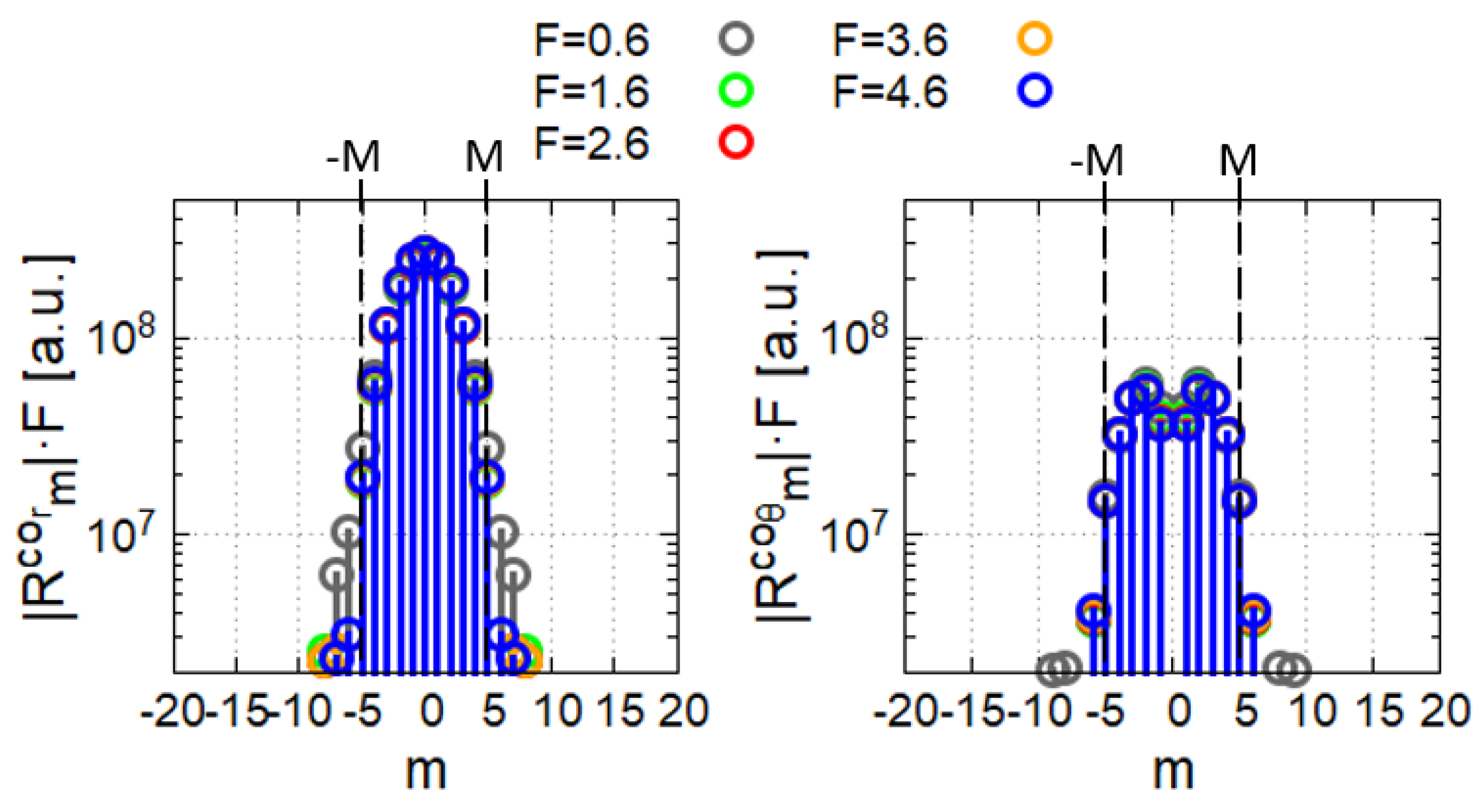
and depend on the field profile and on the kind of roughness on the interface, respectively. Figure 2 shows an example of the FCM AFS. It refers to the y-polarized FCM and is calculated on the boundaries of tube 1 in Figure 1. More details about AFS and AFD can be found in [18]. Even though the spectra of the two components have different shapes, both of them show a "low pass" kind of spectrum, meaning that the AFS coefficients rapidly decrease for increasing m. Values of

m > 5 \div 6

guarantee that the corresponding

R_{m}^{s}

will have values more than one order of magnitude lower than the maximum. The

C_{m}

coefficients depend on the specific perturbation affecting the considered boundary, which will be analyzed in the following sections.

The DM electric field components for a single isolated tube are analytically known [21] and can be written in the following form:

E_{D M}^{s} (r_{0}, θ) = A^{s} e^{j μ θ} .

(6)

By substituting Equations (4), (5), and (6) into Equation (3), and recalling that

\int_{0}^{2 π} e^{- j n θ} d θ = \{\begin{matrix} 0 if n \neq 0 \\ 2 π if n = 0 \end{matrix}

it yields:

k = \frac{q π r_{0}}{η_{0} λ} (n_{d}^{2} - 1) (g^{θ} + g^{r}),

(7)

with

g^{s} = A^{s} \sum_{m} R_{μ - m}^{s} C_{m} .

(8)

2.2. Loss Calculation

Mode coupling, quantified by coefficient k, causes a variation of the FCM attenuation constant. It can be shown that, in that case, the attenuation constant can be written as [22]:

α_{F C M}^{'} = α_{m} - \frac{1}{2} ℑ (\sqrt{{(Δ β - j Δ α)}^{2} + {(2 k)}^{2}}) .

(9)

At the phase matching condition (

Δ β = 0

), under the assumption that

2 | k | < < Δ α

and

α_{F C M_{0}} < < α_{D M_{0}}

, Equation (9) is simplified as:

α_{F C M}^{'} = α_{F C M_{0}} + δ α,

(10)

where

α_{F C M_{0}}

and

α_{D M_{0}}

are the FCM and DM attenuation constants at the phase matching condition in the ideal fiber, respectively, and

δ α = {(\frac{| k |}{α_{D M_{0}}})}^{2}

(11)

is the additional loss due to roughness. By substituting Equation (7) into Equation (11), the expression of the additional loss at the phase matching condition, due to the FCM coupling with a DM as caused by t-roughness, is obtained:

δ α_{i} = {[\frac{D}{λ} (g_{i}^{θ} + g_{i}^{r})]}^{2},

(12)

where

D = π (n_{d}^{2} - 1) r_{0} / (η_{0} α_{D M_{0}})

. The subscript "i" indicates that the quantity refers specifically to the loss increase due to the coupling between the FCM and the i-th DM having polarization either

E H

H E

and indices

μ

and

ν

. When the phase matching condition is not fulfilled, according to Equation (9), the additional loss is reduced and the expression becomes:

δ α^{i} (F) = {[\frac{D}{λ} (g_{i}^{θ} + g_{i}^{r}) L (F - F_{c_{i}})]}^{2},

(13)

where

L (F)

is a normalized function (

L (0) = 1

) which rapidly decreases for increasing F [22] and can be locally approximated by a Lorentzian function [20].

F_{c_{i}}

is the cutoff frequency of the i-th DM.

The total additional loss

α_{t r}

due to t-roughness is the sum of all the contributions:

α_{t r} = \frac{1}{λ^{2}} \sum_{i} {[D_{i} (g_{i}^{θ} + g_{i}^{r}) L (F - F_{c_{i}})]}^{2} .

(14)

The sum is intended to include all DMs and fiber interfaces.

2.3. Scaling Laws

The dependence of

α_{t r}

on the fiber’s parameters is given by Equation (14). According to Equation (8), the contributions of the square of the g parameter scale as

R_{m}^{2}

, which depends on the square of the electric field on the interfaces [18]. The trend of the latter can be effectively estimated by the integral of the square of the electric field on the interfaces

F_{c c}

[4]:

F_{c c} = \sqrt{\frac{ϵ_{0}}{μ_{0}}} \frac{\oint_{Γ} {| \bar{E} |}^{2} d Γ}{{\int \int}_{S_{\infty}} p_{z}} .

(15)

According to an empirical formula, the minimum of

F_{c c}

in each TB scales as

λ^{2} / R_{c o}^{3}

[23]. Combining all the dependencies gives:

α_{t r} \propto \frac{1}{R_{c o}^{3}} .

(16)

This shows that

α_{t r}

does not depend on wavelength, while it rapidly decreases for increasing core size. Since the minimum of CL in each TB in ideal TLFs scales as

λ^{4.5} / R_{c o}^{4}

[23], the effects of t-roughness, compared to those of CL, tend to be more and more significant as wavelength is reduced and core radius is increased.

3. Sinusoidal Corrugation

To gain insight in the coupling mechanism caused by the transverse roughness, it is better to start with a simplified but very useful case. It is shown in the left inset of Figure 1, and it consists of a perfectly sinusoidal perturbation applied only on the inner surface of tube 1:

Δ r (θ) = A_{P} c o s (P θ),

(17)

where P is the number of periods along the tube boundary, resulting in a spatial frequency

{\tilde{f}}_{P} = P / (2 π r_{0})

. Notice that any such kind of perturbation must be periodic within the circumference

2 π r_{0}

and it can always be modeled as a linear superposition of sinusoidal corrugations.

The corresponding AFS has just two nonzero coefficients, for

m = \pm P

C_{P} = C_{- P} = A_{P} / 2

. Substituting them into Equation (8) and then in (12) yields the amplitude of the loss peak, centered at

F = F_{c_{μ, ν}}

δ α_{μ, ν} = D^{2} {(\frac{A_{P}}{2})}^{2} {(A_{μ, ν}^{θ} R_{μ - P}^{θ} + A_{μ, ν}^{r} R_{μ - P}^{r})}^{2} .

(18)

Equation (18) can be further simplified by observing that

E H

polarized DMs have

A_{r} > > A_{θ}

, and the opposite is true for the

H E

ones, so that:

\begin{matrix} δ α_{μ, ν}^{E H} ≃ D^{2} {(\frac{A_{P}}{2})}^{2} {(A_{μ, ν}^{r} R_{μ - P}^{r})}^{2}; \end{matrix}

(19)

\begin{matrix} δ α_{μ, ν}^{H E} ≃ D^{2} {(\frac{A_{P}}{2})}^{2} {(A_{μ, ν}^{θ} R_{μ - P}^{θ})}^{2} . \end{matrix}

(20)

From the previous equations it emerges that, despite the perturbation being purely sinusoidal, the additional loss function

δ α

is composed of a sequence of peaks having amplitude given by Equations (19) and (20), centered at the cutoff frequencies of the involved DMs. The peak amplitudes are shaped by the FCM AFS, "spectrally translated" at the cutoff frequency of the DM with

μ = P

. The number of DMs giving a significant contribution is however limited by the low pass "filtering" given by the FCM AFS. Roughly, only the DMs with

P - M < μ < P + M

for

M = 5 \div 6

give a significant contribution to the additional loss.

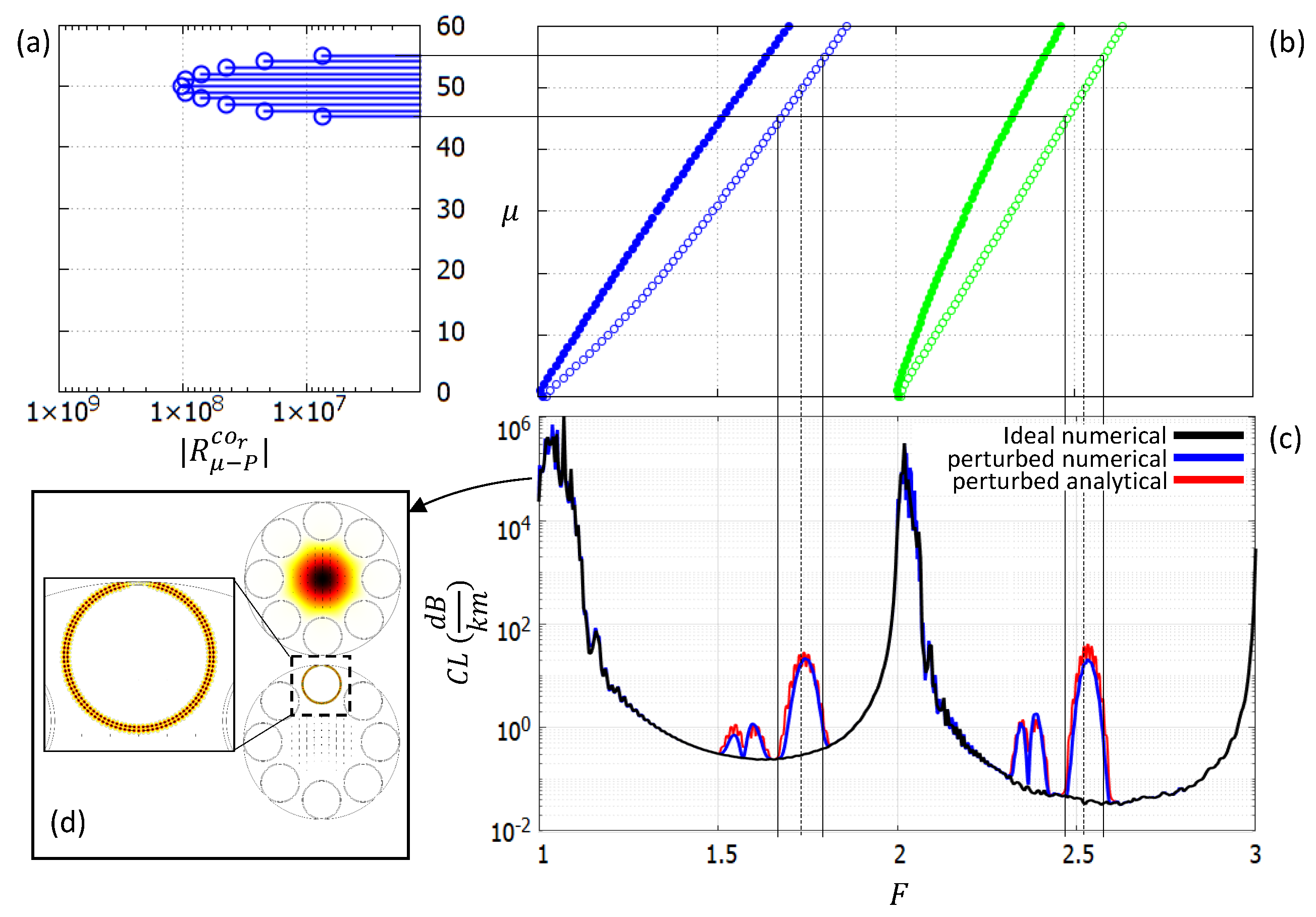
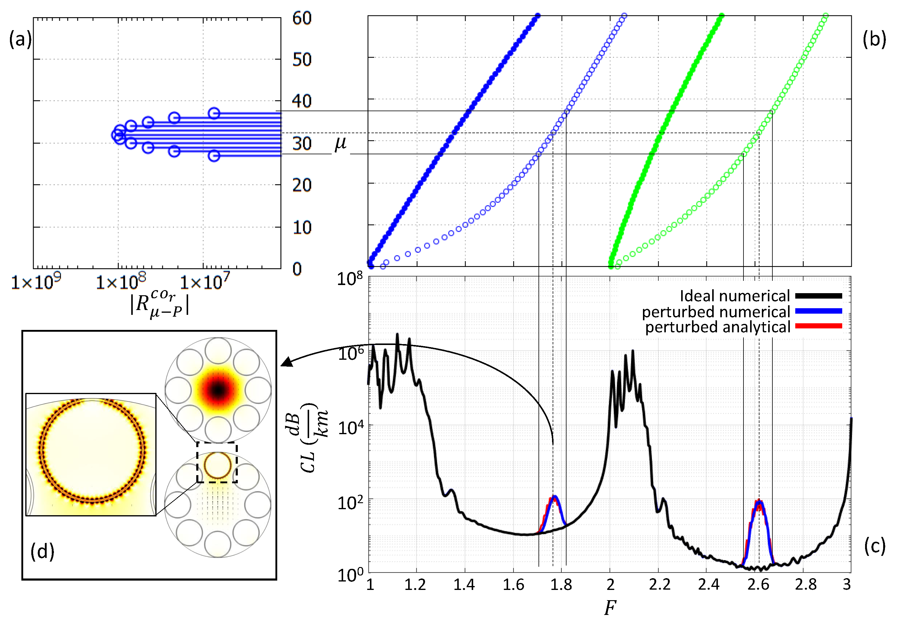
To clarify this concept and validate the model, let us consider Figure 3. It refers to a fiber, hereinafter named Fiber

# 1

, with parameters

R_{c o} = 24.5 μ m

r_{e x t} = 10 μ m

t = 0.5 μ m

n_{d} = 1.45

, and

n_{g} = 1.0

. Panel (c) compares the CL spectra of an ideal and a sinusoidally perturbed fiber with

P = 50

. The two spectra coincide everywhere except for some quite narrow peaks. The peaks here highlighted correspond to the effects of the coupling of the FCM with specific

E H

DMs, given by Equation (19). The loss peak shapes perfectly match the shape of the AFS of the radial component of the FCM (see the left plot in Figure 2), shifted by

m = P = 50

and shown in panel (a). Panel (b) shows the

μ - F_{c}

curves of the DMs, highlighting the correspondence between the azimuthal index

μ

of the DMs and their cutoff frequencies

F_{c_{μ, ν}}

[22]. As we deal with

E H

DMs only, the curves with empty circles must be considered. The correspondence between the coefficients in panel (a) and the spectral collocations of the peaks in panel (c) is very good. The different peaks in the different TBs are due to the coupling of the FCM with DMs having same

μ

but different

ν

. Since the slopes of the

μ - F_{c}

curves increase for increasing

ν

, the peaks change position in the different TBs and shift toward lower frequencies as the order of the TB, and thus the value of

ν

, is increased. Panel (d) shows the real and imaginary part of

{\bar{E}}_{F C M}

F = 1.745

, corresponding to the peak maximum. The imaginary part shows the hybridization with DM

E H_{50, 2}

, that is the one having

μ = P

, due to the coupling, coherently with the theoretical model. Finally, in panel (c) losses obtained from Equation (19) are also reported. The agreement with the numerical results is pretty good.

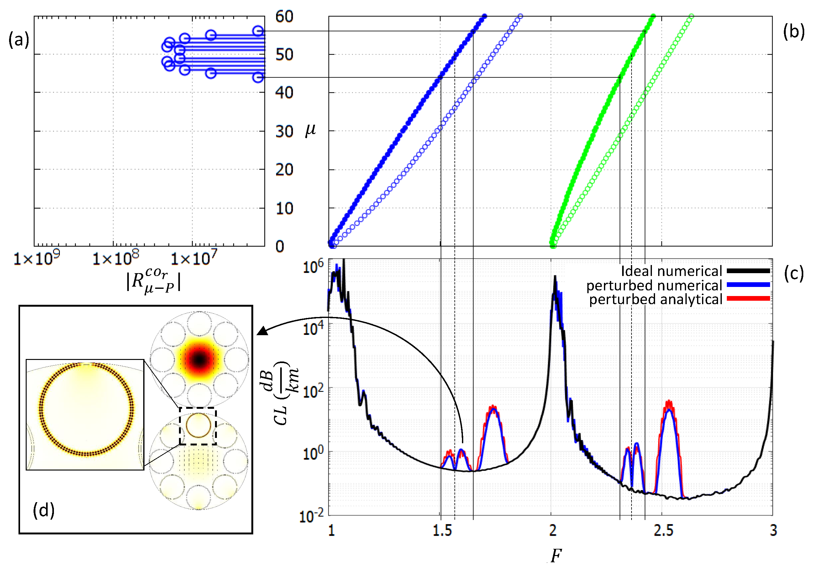
Figure 4 shows the same fiber, in the same condition, but focusing on the coupling with

H E

DMs. According to Equation (20), now the peaks are shaped by the AFS of the FCM azimuthal component (see the right plot in Figure 2), spectrally shifted by

m = P = 50

and shown in panel (a). In this case, the

H E

μ - F_{c}

curves (filled circles) must be considered, and since they have higher slope than the

E H

ones, the peaks are at lower frequencies. Also in this case, the shape of the peaks follows the AFS one and the losses predicted by Equation (20) are again in good agreement with the numerical results.

The amplitudes are lower since the AFS coefficients of the azimuthal FCM component are smaller when compared to the radial ones for the chosen tube and FCM polarization [18]. In

R_{m}^{θ}

, the central coefficient (

m = 0

) is zero, and the maximum of

δ α

occurs for

m = 50

, corresponding to the coupling with DMs

H E_{50, ν}

. Figure 4 shows the FCM filed at

F = 1.6

that is the

F_{c}

H E_{50, 2}

. Once again, the imaginary part shows the hybridization of the FCM with the DM expected by the theoretical model. Similar results are obtained for the x-polarized FCM, just by interchanging the roles of the azimuthal and radial components. It is important to highlight the role played by the

μ - F_{c}

curves. They represent the relationship between the DM indices

μ, ν

and the DM cutoff frequencies

F_{c_{μ, ν}}

, and, in the context of the proposed model, the manner in which the AFS defined in the AFD domain (m index) are mapped to the normalized frequency F domain, resulting in the additional loss spectra.

To complete the analysis and to clarify this crucial aspect, a second fiber (Fiber

# 2

) with the same geometrical parameters as Fiber

# 1

, but having

n_{d} = 2.45

, is analyzed in Figure 5. The change of the dielectric refractive index

n_{d}

significantly modifies the

μ - F_{c}

curves of the

E H

DMs. The same effect, involving in this case both

E H

and

H E

DMs, occurs by changing the tube aspect ratio

ρ = r_{i n t} / r_{e x t}

, but with weaker impact and is not discussed here. The different

μ - F_{c}

curves change the correspondence between azimuthal index and cutoff frequencies, so in order to show peaks in the same TBs, a corrugation with a lower number of periods,

P = 32

, has been considered. The agreement both in terms of shape and spectral collocation is confirmed. Notice that the peaks due to the coupling with

H E

modes are not visible in the perturbed fiber spectrum of Figure 5c. In fact, due to the different shape of the

H E

μ - F_{c}

curves, such peaks fall in the high loss regions and so the effects of

δ α

are negligible.

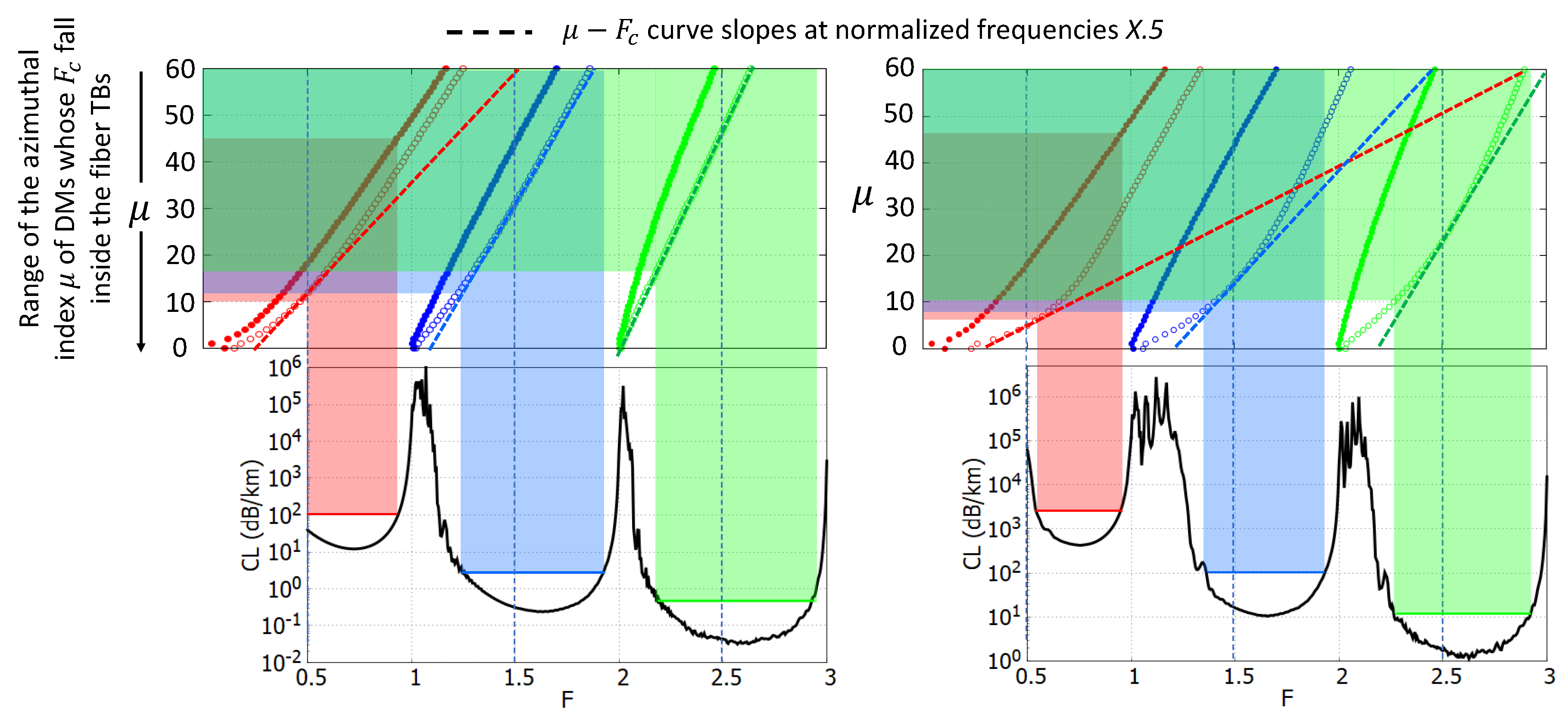
On the basis of those observations, an important result must be highlighted. Recalling that the effects of the corrugation are noticeable only when the peaks fall in the TBs, and that the lobes are quite narrow (

M \sim 5 \div 6

) and are spectrally located at the cutoff frequencies

F_{c_{P, ν}}

of the DMs with

μ = P

, it follows that only the corrugations with spatial period P such that

F_{c_{P, ν}}

falls in TBs cause noticeable additional loss. The concept is illustrated in Figure 6. Just to give a reference, let us define the extension of each TB as the frequency range where losses are lower than ten times the minimum loss for that TB. Light red, light blue and light green regions highlight those ranges and, through the

μ - F_{c}

curves, the P values giving

F_{c_{P, ν}}

within the defined TBs. Even though the values depend on TB spectral extension and

μ - F_{c}

curve slope, speaking in the broadest sense, non negligible contributions occur for

P \geq P_{m i n}

with

P_{m i n} \sim 10

. In terms of spatial frequency

\tilde{f}

, it means that only high spatial frequencies with

\tilde{f} > 10 / (2 π r_{0})

are involved in the loss increase. This has important implications in case of non-sinusoidal perturbations. As will be shown in the next section, it is not the whole spectrum of the t-roughness that is involved, but only its high frequency range.

For the sake of completeness, it must be remarked that, in principle, the spatial periods giving a contribution also have an upper bound, as it can be seen e.g. in Figure 6. As an example, for Fiber #2 in the TB between

F = 1

and

F = 2

, the upper bound corresponds to

P = 50

. However, by taking into account that real PSDs decay for increasing spatial frequency, the upper bounds correspond to spatial frequencies so high that the corresponding roughness spectrum values are very low, enough that they can be neglected in the analysis.

4. Random Corrugation

To take into account the stochastic nature of real roughness, the same treatment proposed in [24] is employed here, but with an adaptation to periodic roughness. Let

Δ r

be a random variable described by a PSD

S (\tilde{f})

where

\tilde{f}

is the spatial frequency. For geometrical reasons,

Δ r

is periodic with a period

2 π r_{0}

and the PSD is thus defined over a discrete set of frequencies

{\tilde{f}}_{P} = m {\tilde{f}}_{0}

which are multiples of the fundamental one

{\tilde{f}}_{0} = 1 / (2 π r_{0})

Δ r

can be written as:

Δ r (θ) = A \sum_{m = 1}^{\infty} \sqrt{S (m {\tilde{f}}_{0})} cos (m θ + ϕ_{P})

(21)

where

ϕ_{m}

is a random variable uniformly distributed between 0 and

2 π

. By exploiting Euler’s formula:

cos (m θ + ϕ_{m}) = 1 / 2 e^{j ϕ_{m}} e^{j m θ} + 1 / 2 e^{- j ϕ_{m}} e^{- j m θ}

, the

C_{m}

coefficients in Equation (8) can be written with the following expression:

C_{m} = \frac{A}{2} \sqrt{S (m {\tilde{f}}_{0})} e^{- j ϕ_{m} m / | m |} .

(22)

The loss calculation for TLFs affected by random t-roughness is obtained by applying a independent random corrugation on each tube interface, by performing ten independent simulations, and by calculating the average value for each frequency.

First of all, let us consider a "white" random roughness, that is one described by a constant PSD:

S (\tilde{f}) = S_{0} \forall \tilde{f} .

(23)

An example is shown in Figure 7a where

S_{0} = 6 \cdot 10^{- 3} n m

. Even though it corresponds to a non-physical process, as the corresponding Root Mean Square (RMS) value is infinite, this process is useful to separate the frequency dependence of the FCM-DM coupling from the PSD one.

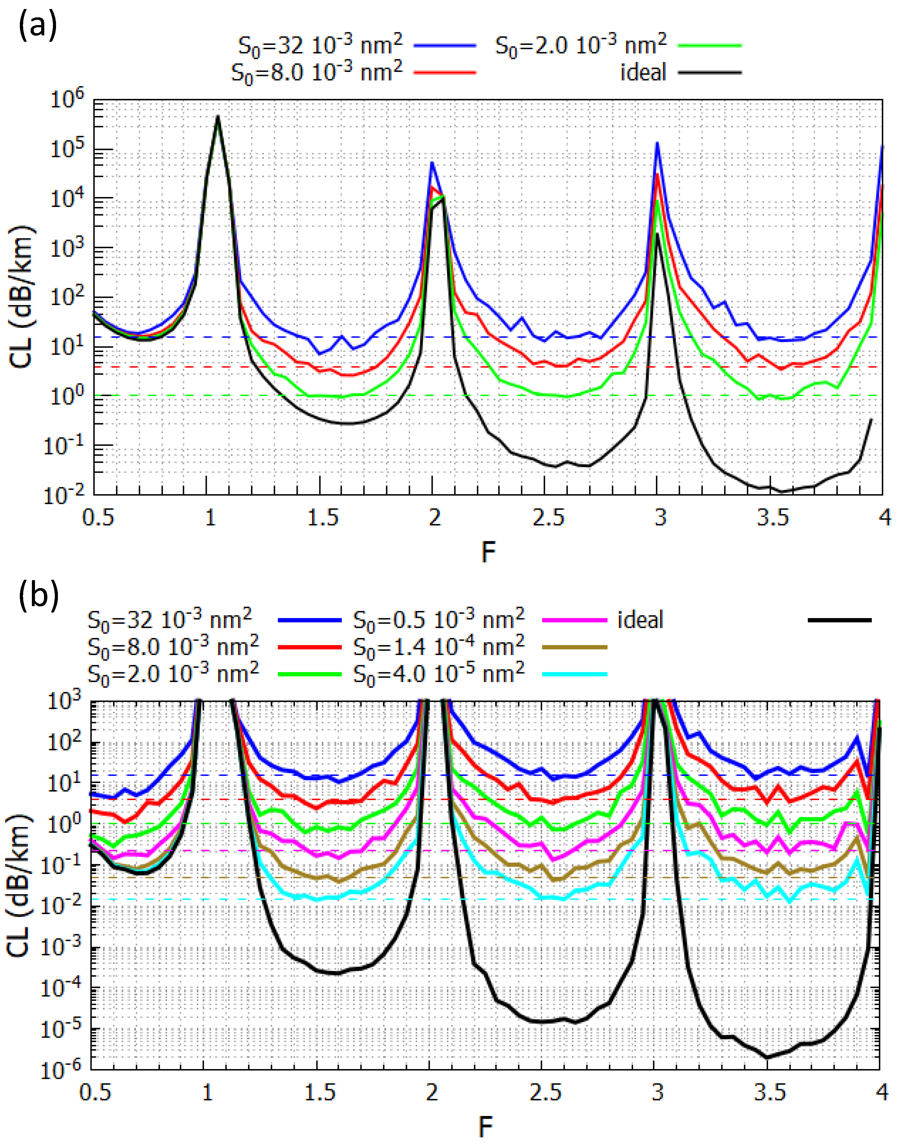
Figure 8 compares the loss of the ideal Fiber

# 1

and the same with t-roughness, and a nested fiber with the same geometrical parameters and

r_{n e s t e d} = 0.5 r_{e x t}

, for different values of

S_{0}

. With the exception of the fundamental TB, for a given

S_{0}

the TB minima have almost the same values irrespective of the TB order. This is coherent with the discussion of the scaling laws from Section 2.3 and Equation (16). The minima values are also independent of the kind of the fiber (TLF or nested). In fact, according to Equation (11), the additional loss

δ α

does not depend on the FCM loss of the ideal fiber. Finally, as expected by the model,

α_{t r}

is directly proportional to

S_{0}

(see Equations (8), (12), and (22)). For the considered fiber, the relationship is:

δ α (d B / k m) = 500 S_{0} (n m^{2}) .

(24)

The effects of t-roughness are negligible if

α_{t r} < α_{F C M_{0}}

. Propagation losses lower than

0.1 d B / k m

are just a step ahead in the near infrared region [3]. With those values, t-roughness effects are negligible if the PSD value is lower than

2 \cdot 10^{- 4} n m^{2}

The Fundamental TB (FTB) is a different matter. In the TLF,

α_{F C M_{0}}

is higher than any

α_{t r}

corresponding to the

S_{0}

here considered, thus the t-roughness effects are not observable. The effects are visible in the nested fiber and the minima values are lower than those of the other TBs. This is in contrast with the scaling laws discussed in Section 2.3 and the trends in the other TBs. To understand this apparent anomaly, it is necessary to recall that the final value of

α_{t r}

is also given by the contribution of the lateral tails of the function

L (F)

. When DM contributions

δ α_{i}

are spectrally dense (the

F_{c_{i}}

are very close each other) each peak is overlapping with the tails of a number of adjacent peaks. If the spectral density is reduced, the same happens for the tail overlap and

α_{t r}

. Observing the

μ - F_{c}

curves in the first TB (corresponding to radial index

ν = 0

), the slopes are lower than those of higher order TBs [4], resulting in a lower spectral density of DMs and a lower

α_{t r}

White PSD cannot describe a real roughness. There are different proposals about the roughness PSD in hollow core fibers. Here we consider a stochastic process with an exponential auto-correlation function having correlation length

L_{c}

. The corresponding PSD is:

S (m {\tilde{f}}_{0}) = σ^{2} \frac{r_{0}}{m_{c}} \frac{1}{1 + {(\frac{m}{2 π m_{c}})}^{2}},

(25)

where

σ

is the RMS value, and

m_{c}

is the cutoff parameter such that

{\tilde{f}}_{m_{c}} = {\tilde{f}}_{c} = 1 / (2 π L_{c})

. An example with parameters

σ = 1 n m

m_{c} = 40

, and

r_{0} = 12 μ m

is shown in Figure 7(b). For low spatial frequencies (

\tilde{f} < {\tilde{f}}_{c}

), the PSD is approximately constant, whereas for

\tilde{f} > {\tilde{f}}_{c}

it tends to decay with a rate of

1 / {\tilde{f}}^{2}

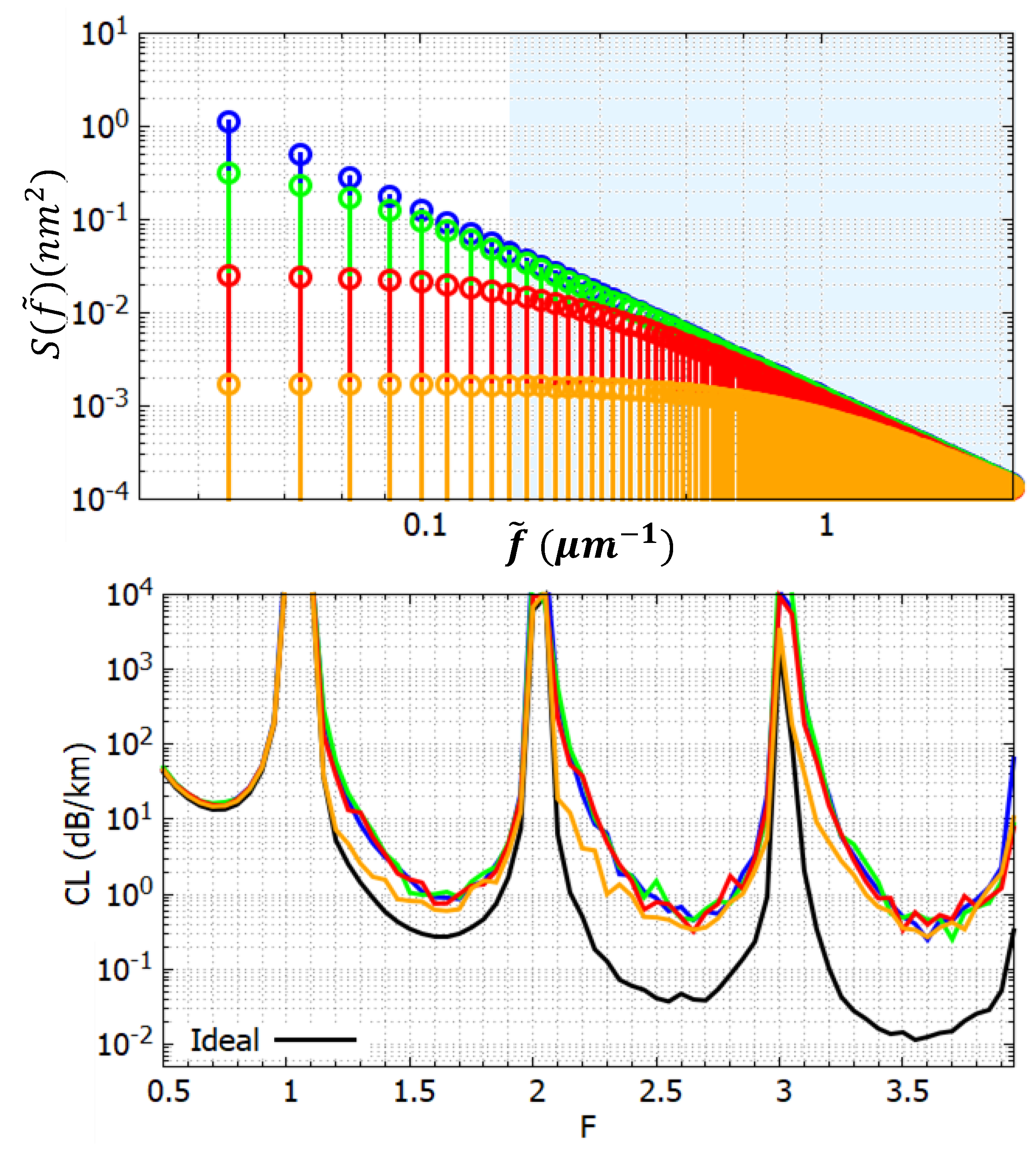
. As highlighted in the previous section, not all the spatial frequencies contribute to the additional loss in the TBs. To validate this results also in the case of random roughness, Fiber

# 1

has been investigated by considering different PSDs having different

σ

, and different cutoff

m_{c}

, but the same values at high frequencies. The results are shown in Figure 9. The light-blue area shows the spectral range where

m \geq 10

, which refers approximately to the spectral components acting on the TBs. Three PSDs have almost the same values in this range, whereas the fourth has a lower value up to

m \sim 25

The losses caused by the fist three PSD functions are almost perfectly overlapping. The fourth shows lower values up to the center of the TBs and reaches the same values as the others in the second half of the TBs, corresponding to the cutoffs of DMs having

μ \geq 25

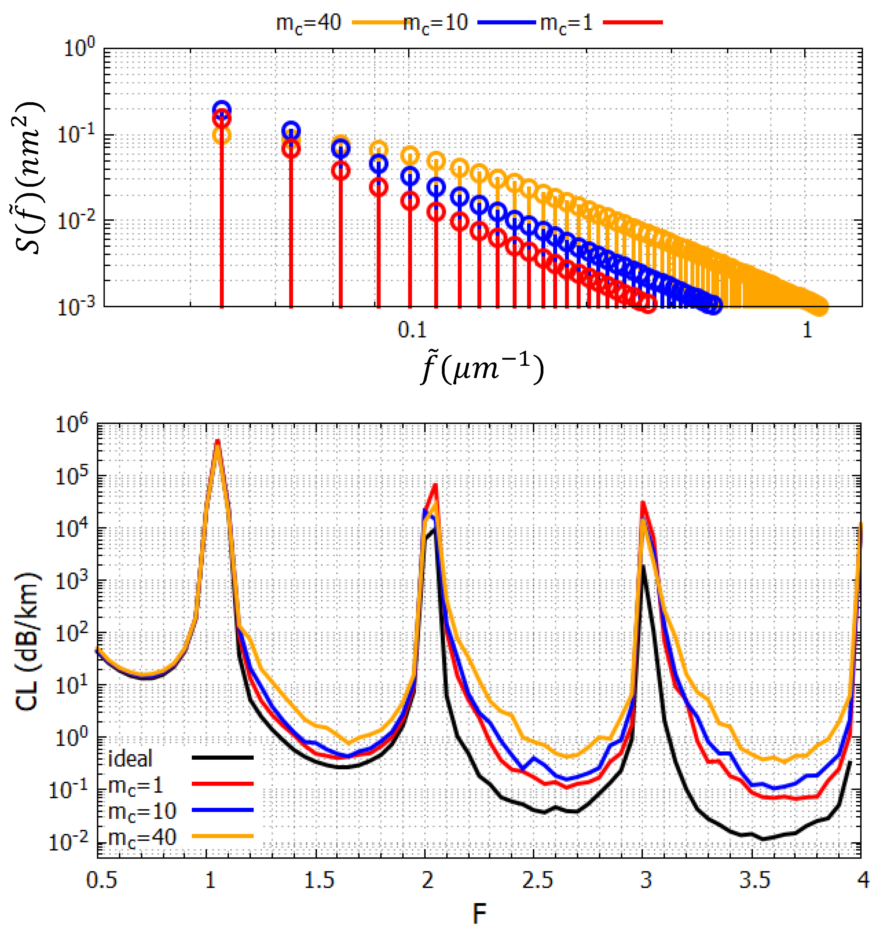
Results agree perfectly with the model and confirm that the losses caused by t-roughness are not directly related to either the RMS value or the cutoff, but only to the PSD values at high spatial frequencies. PSD values at low frequencies do not play any role in defining the loss caused by t-roughness. Figure 10 compares the effects of PSDs having the same RMS

σ = 1.0 n m

and different cutoffs

m_{c} = 1, 10, 40

. As expected, the loss enhancement is not proportional to

m_{c}

, because the PSD values at high frequencies are not. In particular, notice that by comparing the PSDs having

m_{c} = 1

and

m_{c} = 40

, the former has much higher values at low frequencies than the latter, but the corresponding losses are lower, since the values at high frequencies are.

5. Conclusions

In this work, a model for the analysis and investigation of the effects of tube surface roughness along the transverse direction in HC-TLFs has been proposed and validated. The model is based on coupled mode theory and azimuthal Fourier decomposition, and it shows that roughness causes additional loss through the coupling between FCM and DMs. It has been validated by considering both a deterministic sinusoidal corrugation and a stochastic roughness with exponential autocorrelation function. The theory is in agreement with the numerical results, showing that the additional loss depends on the spectral content of the t-roughness PSD at high frequencies irrespective of the RMS value, that it scales as the inverse of the cube of the core radius, and that it is independent of the wavelength. Fibers with low loss in the ideal case, such as nested ones, are especially sensitive to t-roughness. To guarantee that t-roughness effects are negligible even for losses lower than 0.1 dB/km, the PSD at spatial frequencies higher than

10 / (2 π r_{0})

should be lower than 0.2 nm².

References

Osório, J.H.; Amrani, F.; Delahaye, F.; Dhaybi, A.; Vasko, K.; Melli, F.; Giovanardi, F.; Vandembroucq, D.; Tessier, G.; Vincetti, L.; Debord, B.; Gérôme, F.; Benabid, F. Hollow-core fibers with reduced surface roughness and ultralow loss in the short-wavelength range. Nat. Comm. 2023, 14, 1146. [Google Scholar] [CrossRef] [PubMed]
Jasion, G.; Sakr, H.; Hayes, J.; Sandoghchi, S.; Hooper, L.; Numkam Fokoua, E.; Saljoghei, A.; Mulvad, H.; Alonso, M.; Taranta, A.; Bradley, T.; Davidson, I.A.; Chen, Y.; Richardson, D.; Poletti, F. 0.174 dB/km Hollow Core Double Nested Antiresonant Nodeless Fiber (DNANF). 2022 Optical Fiber Communications Conference and Exhibition (OFC), 2022, pp. 1–3.
Chen, Y.; Petrovich, M.; Fokoua, E.N.; Adamu, A.I.; Hassan, M.R.B.A.; Sakr, H.; shahab Bakhtiari, Gorajoobi; Alonso, M.; Ando, R.F.; Papadimopoulos, A.; Varghese, T.; Wu, D.; Ando, M.F.; Wisniowski, K.; Sandoghchi, S.R.; Jasion, G.T.; Richardson, D.J.; Poletti, F.; Slavik, R. Hollow Core DNANF Optical Fiber with < 0.11 dB/km Loss. 2024 Optical Fiber Communications Conferenceand Exhibition (OFC), 2024, pp. 1–3.
Melli, F.; Rosa, L.; Vasko, K.; Benabid, F.; Vincetti, L. Loss Modeling and Analysis in Hollow-Core Inhibited-Coupling Fibers. submitted to Journal of Lightwave Technology 2024. [Google Scholar]
Wang, Y.Y.; Wheeler, N.V.; Couny, F.; Roberts, P.J.; Benabid, F. Low loss broadband transmission in hypocycloid-core Kagome hollow-core photonic crystal fiber. Opt. Lett. 2011, 36, 669–671. [Google Scholar] [CrossRef] [PubMed]
Vincetti, L.; Setti, V.; Zoboli, M. Terahertz Tube Lattice Fibers With Octagonal Symmetry. IEEE Photonics Technology Letters 2010, 22, 972–974. [Google Scholar] [CrossRef]
Pryamikov, A.D.; Biriukov, A.S.; Kosolapov, A.F.; Plotnichenko, V.G.; Semjonov, S.L.; Dianov, E.M. Demonstration of a waveguide regime for a silica hollow-core microstructured optical fiber with a negative curvature of the core boundary in the spectral region > 3.5 μm. Opt. Express 2011, 19, 1441–1448. [Google Scholar] [CrossRef] [PubMed]
Belardi, W.; Knight, J.C. Negative curvature fibers with reduced leakage loss. OFC 2014, 2014, 1–3. [Google Scholar] [CrossRef]
Poletti, F. Nested antiresonant nodeless hollow core fiber. Opt. Express 2014, 22, 23807–23828. [Google Scholar] [CrossRef] [PubMed]
Gao, S.f.; Wang, Y.y.; Ding, W.; Jiang, D.l.; Gu, S.; Zhang, X.; Wang, P. Hollow-core conjoined-tube negative-curvature fibre with ultralow loss. Nature Communications 2018, 9, 2828. [Google Scholar] [CrossRef] [PubMed]
Amrani, F.; Osório, J.H.; Delahaye, F.; Giovanardi, F.; Vincetti, L.; Debord, B.; Gérôme, F.; Benabid, F. Low-loss single-mode hybrid-lattice hollow-core photonic-crystal fibre. Light Sci. Appl. 2021, 10, 7. [Google Scholar] [CrossRef] [PubMed]
Melli, F.; Rosa, L.; Vincetti, L. Analytical Formulas for Micro-Bending and Surface Scattering Loss Estimation in Tube Lattice Fibers. Journal of Lightwave Technology 2023, 41, 5714–5721. [Google Scholar] [CrossRef]
Fokoua, E.N.; Mousavi, S.A.; Jasion, G.T.; Richardson, D.J.; Poletti, F. Loss in hollow-core optical fibers: mechanisms, scaling rules, and limits. Adv. Opt. Photon. 2023, 15, 1–85. [Google Scholar] [CrossRef]
Roberts, P.J.; Couny, F.; Sabert, H.; Mangan, B.J.; Williams, D.P.; Farr, L.; Mason, M.W.; Tomlinson, A.; Birks, T.A.; Knight, J.C.; Russell, P.S. Ultimate low loss of hollow-core photonic crystal fibres. Opt. Express 2005, 13, 236–244. [Google Scholar] [CrossRef] [PubMed]
Bresson, B.; Brun, C.; Buet, X.; Chen, Y.; Ciccotti, M.; Gâteau, J.; Jasion, G.; Petrovich, M.N.; Poletti, F.; Richardson, D.J.; Sandoghchi, S.R.; Tessier, G.; Tyukodi, B.; Vandembroucq, D. Anisotropic Superattenuation of Capillary Waves on Driven Glass Interfaces. Phys. Rev. Lett. 2017, 119, 235501. [Google Scholar] [CrossRef] [PubMed]
Melli, F.; Vasko, K.; Rosa, L.; Vincetti, L.; Benabid, F. Transverse Roughness Effect on Fundamental Mode Confinement Loss and Modal Content of Hollow-Core Inhibited Coupling Tube Lattice Fibers. Optica Advanced Photonics Congress 2022. Optica Publishing Group, 2022, p. SoTu1I.3. [CrossRef]
Melli, F.; Vasko, K.; Rosa, L.; Benabid, F.; Vincetti, L. Transverse Roughness: Modeling and Effects Analysis on Inhibited Coupling Fibers. Advanced Photonics Congress 2024. Optica Publishing Group, 2024, p. SoM3F.6. [CrossRef]
Melli, F.; Vasko, K.; Rosa, L.; Benabid, F.; Vincetti, L. Azimuthal Fourier decomposition for loss analysis of hollow-core tube lattice fibers part I: Ideal fibers. Results in Optics 2024, 15, 100657. [Google Scholar] [CrossRef]
Melli, F.; Giovanardi, F.; Vasko, K.; Rosa, L.; Benabid, F.; Vincetti, L. Azimuthal Fourier decomposition for loss analysis of hollow-core tube lattice fibers, Part II: Tube thickness variation effects. Results in Optics 2024, 16, 100726. [Google Scholar] [CrossRef]
Vincetti, L.; Rosa, L. A simple analytical model for confinement loss estimation in hollow-core Tube Lattice Fibers. Opt. Express 2019, 27, 5230–5237. [Google Scholar] [CrossRef] [PubMed]
Kharadly, M.; Lewis, J. Properties of dielectric-tube waveguides. Proceedings of the Institution of Electrical Engineers 1969, 116, 214–224. [Google Scholar] [CrossRef]
Melli, F.; Rosa, L.; Vasko, K.; Benabid, F.; Vincetti, L. Modeling of the Mode Couplings in Hollow-Core Inhibited-Coupling Fibers. submitted to Journal of Lightwave Technology 2024. [Google Scholar]
Vincetti, L. Empirical formulas for calculating loss in hollow core tube lattice fibers. Opt. Express 2016, 24, 10313–10325. [Google Scholar] [CrossRef] [PubMed]
Jin, X.; Payne, F.P. Numerical Investigation of Microbending Loss in Optical Fibres. Journal of Lightwave Technology 2016, 34, 1247–1253. [Google Scholar] [CrossRef]

Figure 1. Top: Fiber cross-section with geometrical parameters. Gray regions refer to dielectric with refractive index

n_{d}

, white ones to a material with

n_{g} = 1

. The right inset shows an example of a tube whose boundaries are affected by transverse roughness, together with the employed local polar frame of reference. The left inset shows a tube with only the inner boundary affected by a perfect sinusoidal corrugation. Bottom: detail of the surface with random roughness and representation in terms of the local polar frame of reference and the displacement

Δ r (θ)

Figure 1. Top: Fiber cross-section with geometrical parameters. Gray regions refer to dielectric with refractive index

n_{d}

, white ones to a material with

n_{g} = 1

Δ r (θ)

Figure 2. AFS of the radial (left) and azimuthal (right) components of the FCM, calculated at the inner and outer boundaries of tube 1 for different normalized frequencies.

Figure 3. Fiber

# 1

having a sinusoidal perturbation with amplitude

A_{P} = 0.005 t

and number of periods

P = 50

. (a): Azimuthal spectrum of the y-polarized FM azimuthal component. (b): Azimuthal index

μ

versus cutoff frequency

F_{c}

H E

(filled circles) and

E H

(empty circles) DMs having

ν = 2

(blue) and

ν = 3

(green). (c): CL spectra of the ideal (black) and perturbed (red) fiber. (d): Real and imaginary part of the FM electric field of the perturbed fiber calculated at frequency

F = 1.745

, corresponding to the cutoff frequency of the

E H_{50, 2}

mode. The inset shows a detail of the perturbed tube.

Figure 3. Fiber

# 1

having a sinusoidal perturbation with amplitude

A_{P} = 0.005 t

and number of periods

P = 50

. (a): Azimuthal spectrum of the y-polarized FM azimuthal component. (b): Azimuthal index

μ

versus cutoff frequency

F_{c}

H E

(filled circles) and

E H

(empty circles) DMs having

ν = 2

(blue) and

ν = 3

(green). (c): CL spectra of the ideal (black) and perturbed (red) fiber. (d): Real and imaginary part of the FM electric field of the perturbed fiber calculated at frequency

F = 1.745

, corresponding to the cutoff frequency of the

E H_{50, 2}

mode. The inset shows a detail of the perturbed tube.

Figure 4. Fiber

# 1

having a sinusoidal perturbation with amplitude

A_{P} = 0.005 t

and number of periods

P = 50

. (a): Azimuthal spectrum of the y-polarized FM azimuthal component. (b): Azimuthal index

μ

versus cutoff frequency

F_{c}

H E

(filled circles) and

E H

(empty circles) DMs having

ν = 2

(blue) and

ν = 3

(green). (c): CL spectra of the ideal (black) and perturbed (red) fiber. (d): Real and imaginary part of the FM electric field of the perturbed fiber calculated at frequency

F = 1.6

, corresponding to the cutoff frequency of the

H E_{50, 2}

mode. The inset shows a detail of the perturbed tube.

Figure 4. Fiber

# 1

having a sinusoidal perturbation with amplitude

A_{P} = 0.005 t

and number of periods

P = 50

. (a): Azimuthal spectrum of the y-polarized FM azimuthal component. (b): Azimuthal index

μ

versus cutoff frequency

F_{c}

H E

(filled circles) and

E H

(empty circles) DMs having

ν = 2

(blue) and

ν = 3

(green). (c): CL spectra of the ideal (black) and perturbed (red) fiber. (d): Real and imaginary part of the FM electric field of the perturbed fiber calculated at frequency

F = 1.6

, corresponding to the cutoff frequency of the

H E_{50, 2}

mode. The inset shows a detail of the perturbed tube.

Figure 5. Fiber

# 2

having a sinusoidal perturbation with amplitude

A_{P} = 0.05 t

and number of periods

P = 32

. (a): Azimuthal spectrum of the y-polarized FM azimuthal component. (b): Azimuthal index

μ

versus cutoff frequency

F_{c}

H E

(filled circles) and

E H

(empty circles) DMs having

ν = 2

(blue) and

ν = 3

(green). (c): CL spectra of the ideal (black) and perturbed (red) fiber. (d): Real and imaginary part of the FM electric field of the perturbed fiber calculated at frequency

F = 1.765

, corresponding to the cutoff frequency of the

E H_{32, 2}

mode. The inset shows a detail of the perturbed tube.

Figure 5. Fiber

# 2

having a sinusoidal perturbation with amplitude

A_{P} = 0.05 t

and number of periods

P = 32

. (a): Azimuthal spectrum of the y-polarized FM azimuthal component. (b): Azimuthal index

μ

versus cutoff frequency

F_{c}

H E

(filled circles) and

E H

(empty circles) DMs having

ν = 2

(blue) and

ν = 3

(green). (c): CL spectra of the ideal (black) and perturbed (red) fiber. (d): Real and imaginary part of the FM electric field of the perturbed fiber calculated at frequency

F = 1.765

, corresponding to the cutoff frequency of the

E H_{32, 2}

mode. The inset shows a detail of the perturbed tube.

Figure 6. Spatial period ranges involved in the TBs of Fibers

# 1

(left) and

# 2

(right). Red, blue and green colored regions show how the TBs (bottom) are linked to the spatial periods through the

μ - F_{c}

curves (top). In particular, only perturbations with a number of periods

P = μ

greater than 10 give a TB loss contribution. Dashed kines show the

μ - F_{c}

curve slopes at the normalized frequencies

F = 0.5, 1.5, 2.5

Figure 6. Spatial period ranges involved in the TBs of Fibers

# 1

(left) and

# 2

(right). Red, blue and green colored regions show how the TBs (bottom) are linked to the spatial periods through the

μ - F_{c}

curves (top). In particular, only perturbations with a number of periods

P = μ

greater than 10 give a TB loss contribution. Dashed kines show the

μ - F_{c}

curve slopes at the normalized frequencies

F = 0.5, 1.5, 2.5

Figure 7. PSD versus spatial frequency. (a) "White" roughness. (b) Roughness having an exponential autocorrelation function.

Figure 8. Fibers affected by t-roughness with "white" PSD. Losses of (a) Fiber

# 1

and of (b) the corresponding nested TLF having

r_{n e s t e d} = 0.5 r_{e x t}

are reported for different

S_{0}

values and for the ideal TLFs. Dashed lines highlight the loss minima values for each

S_{0}

value, obtained from Equation (24).

Figure 8. Fibers affected by t-roughness with "white" PSD. Losses of (a) Fiber

# 1

and of (b) the corresponding nested TLF having

r_{n e s t e d} = 0.5 r_{e x t}

are reported for different

S_{0}

values and for the ideal TLFs. Dashed lines highlight the loss minima values for each

S_{0}

value, obtained from Equation (24).

Figure 9. Fiber

# 1

affected by t-roughness with different RMS

σ

and cutoff

m_{c}

, but the same PSD for

P > 10

except for the orange one. PSD parameters are:

σ = 2.7 n m

and

m_{c} = 1

(blue);

σ = 1.4 n m

and

m_{c} = 20

(green);

σ = 0.7 n m

and

m_{c} = 80

(red);

σ = 0.35 n m

and

m_{c} = 330

(orange). Top: PSD functions. Bottom: Losses of the ideal TLF and of the one affected by t-roughness. Same colors refer to same PSD parameters.

Figure 9. Fiber

# 1

affected by t-roughness with different RMS

σ

and cutoff

m_{c}

, but the same PSD for

P > 10

except for the orange one. PSD parameters are:

σ = 2.7 n m

and

m_{c} = 1

(blue);

σ = 1.4 n m

and

m_{c} = 20

(green);

σ = 0.7 n m

and

m_{c} = 80

(red);

σ = 0.35 n m

and

m_{c} = 330

(orange). Top: PSD functions. Bottom: Losses of the ideal TLF and of the one affected by t-roughness. Same colors refer to same PSD parameters.

Figure 10. Fiber

# 1

affected by t-roughness having

σ = 1.0 n m

and three different cutoffs:

m_{c} = 1, 10, 40

. Top: PSD functions. Bottom: loss of the ideal TLF and of the TLFs affected by the corresponding t-roughness.

Figure 10. Fiber

# 1

affected by t-roughness having

σ = 1.0 n m

and three different cutoffs:

m_{c} = 1, 10, 40

. Top: PSD functions. Bottom: loss of the ideal TLF and of the TLFs affected by the corresponding t-roughness.

Disclaimer/Publisher’s Note: The statements, opinions and data contained in all publications are solely those of the individual author(s) and contributor(s) and not of MDPI and/or the editor(s). MDPI and/or the editor(s) disclaim responsibility for any injury to people or property resulting from any ideas, methods, instructions or products referred to in the content.

© 2024 by the authors. Licensee MDPI, Basel, Switzerland. This article is an open access article distributed under the terms and conditions of the Creative Commons Attribution (CC BY) license (http://creativecommons.org/licenses/by/4.0/).

Copyright: This open access article is published under a Creative Commons CC BY 4.0 license, which permit the free download, distribution, and reuse, provided that the author and preprint are cited in any reuse.

Alerts

MDPI Initiatives

Important Links

Choose an area of interest and we will send you notifications of new preprints at your preferred frequency.

Disclaimer

Modelling and Analysis of the Transverse Surface Roughness in Hollow Core Fibers

Abstract

Keywords:

Subject:

1. Introduction

2. Modeling

2.1. Coupling Coefficient Calculation

2.2. Loss Calculation

2.3. Scaling Laws

3. Sinusoidal Corrugation

4. Random Corrugation

5. Conclusions

References

MDPI Initiatives

Important Links

Subscribe