
Submitted:
22 October 2024
Posted:
22 October 2024
You are already at the latest version
Abstract
Graph neural networks (GNNs) have been effectively implemented in a variety of real-world applications, while their underlying work mechanisms remain a mystery. To unveil this mystery and advocate trustworthy decision-making, many GNN explainers have been proposed. However, existing explainers often face significant challenges, such as: 1) explanations being tied to specific instances; 2) limited generalizability to unseen graphs; 3) potential generation of invalid graph structures; and 4) restrictions to particular tasks (e.g., node classification, graph classification). To address these challenges, we propose a novel explainer, GAN-GNNExplainer, which employs a generator to produce explanations and a discriminator to oversee the generation process, enhancing the reliability of the outputs. Despite its advantages, GAN-GNNExplainer still struggles with generating faithful explanations and underperforms on real-world datasets. To overcome these shortcomings, we introduce ACGAN-GNNExplainer, an improved approach that improves upon GAN-GNNExplainer by using a more robust discriminator that consistently monitors the generation process, thereby producing explanations that are both reliable and faithful. Extensive experiments on both synthetic and real-world graph datasets demonstrate the superiority of our proposed methods over existing GNN explainers.
Keywords:
Graph Neural Networks
; Explanations
; Generative Methods
; Faithful
; Reliable
1. Introduction
Graph neural networks (GNNs) have swiftly progressed as a powerful method for processing graph-structured data, showing outstanding performance across various real-world applications, including crime prediction [1], traffic flow estimation [2], event forecasting [3], and medical diagnosis [4]. GNNs are proficient in capturing intricate node relationships and extracting valuable features from graph data, making them an ideal option for tasks that require graph-based analysis.
Although GNNs demonstrate strong performance, their lack of explainability reduces their trustworthiness in key fields like healthcare and finance. The inherent black-box characteristic of GNNs complicates the comprehension of their decision-making mechanisms, making it challenging to uncover the reasoning behind their predictions and to detect potential biases. These challenges have restricted the wider adoption of GNNs in vital sectors where interpretability and transparency are essential, including healthcare [5], recommendation systems [6], and other areas.
To address this challenge, a multitude of GNN explainers have been proposed to shed light on the decision-making process of GNNs. These methods provide explanations at the node or graph level, helping to identify important graph structures and features that contribute to the model’s predictions. Specifically, explaining GNN models is encouraged and even required to increase confidence in the GNN model’s predictions, guarantee the security of real-world applications, and promote trustworthy artificial intelligence (AI) [7,8].
The explanation of GNN has attracted substantial scholarly interest, and many explainers [9,10,11,12,13] have been proposed over the past few years. Although these methods provide some useful explanations for complex GNN models, their practical application is hampered by their inherent constraints— 1) the explanation scale is tied to a specific instance; 2) the explanation cannot be easily generalised for unseen graphs; 3) the explanation may not be a valid graph; 4) the explanation may limit to a specific task (e.g., node classification, graph classification, etc.). In particular, the seminal method GNNExplainer [9] limits itself to local explanation and lacks the generalizability. After that, XGNN [11], which trains a graph generator to explain a class by displaying class-specific graph patterns, addressed the limitation of the explanation scale. However, it still lacks the generalizability, and worse, it may generate some nonexisting important subgraphs. Recent Gem [13] has mitigated the limitations faced by previous methods, while its precision in explaining different tasks can vary significantly and lacks stability due to the inherent nature of the generation process.
To tackle the existing limitations, this paper introduces two novel GNN explainers, GAN-GNNExplainer and ACGAN-GNNExplainer, respectively, which use the generative method to produce explanations for GNNs. Both of our methods consist of a generator and a discriminator. In special, for GAN-GNNExplainer, the generator learns to produce explanations for the input graph , which requires an explanation. Meanwhile, the discriminator distinguishes between “real" and generated explanations. The discriminator provides feedback to the generator, refining the explanation process. Through repeated interactions between the generator and discriminator, the generator eventually produces explanations that closely resemble the desired “real" ones. As a result, the quality of the explanations improves, leading to a significant boost in overall explanation accuracy. Even GAN-GNNExplainer represents a notable advancement in the accuracy of explanations, successfully addressing some limitations of current popular GNN explainers. However, GAN-GNNExplainer has inadequate reliability on real-world datasets and lacks fidelity.
To address these limitations, we introduce an enhanced method, ACGAN-GNNExplainer, which leverages the Auxiliary Classifier Generative Adversarial Network (ACGAN) [14] as its backbone to generate explanations for GNNs. Specifically, the input graph , along with its corresponding label , determined by the target GNN model f, is fed into the generator, which then learns to generate explanations. To ensure the validity and accuracy of the generated subgraph, a discriminator is incorporated. The discriminator distinguishes between “real” and generated explanations, assigns a prediction label to each explanation, and provides feedback to the generator, overseeing the entire generation process. Through extensive experimentation on both synthetic and real-world datasets, we demonstrate the effectiveness of our method, showcasing its superiority over existing GNN explainers.
Key contributions of this paper include:
- We propose a novel explainer called GAN-GNNExplainer, specifically tailored for GNN models. This approach employs a generator to generate explanations and is supervised by a discriminator, ensuring reliable results throughout the procedure.
- Additionally, we introduce ACGAN-GNNExplainer, a more advanced explainer for GNN models. It leverages both a generator and a discriminator, which consistently oversees the procedure, leading to explanations that are both reliable and faithful.
- Our methods are comprehensively evaluated across various graph datasets, spanning both synthetic and real-world data, and across multiple tasks, including node classification and graph classification. The outcomes consistently highlight the advantages of our approach over existing methods.
2. Related Work
2.1. Generative Adversarial Networks
Generative Adversarial Networks (GANs) [15] are composed of two main components: a generator and a discriminator, both of which are trained concurrently in a competitive setup. The generator begins with random noise and learns to create synthetic samples that closely resemble the real data distribution, while the discriminator distinguishes between genuine data and synthetic outputs generated by the generator. During the training process, the generator aims to produce increasingly realistic outputs, making it progressively difficult for the discriminator to differentiate them accurately. This adversarial mechanism has allowed GANs to make remarkable advancements in multiple fields, including image synthesis, data augmentation, and cross-modal tasks.
Over time, a variety of GAN extensions have been developed, addressing issues such as training stability and mode collapse, while also improving the diversity and fidelity of the generated outputs. These innovations involve alterations to network architectures, loss functions, and optimization strategies. For instance, conditional GANs (CGANs) [16] introduce a conditioning mechanism, where additional information (such as class labels) is provided to both the generator and discriminator, enabling the generation of class-specific samples. This conditional setup allows for more targeted generation tasks, improving sample diversity and applicability.
In another line of work, models such as InfoGAN [17] explore the disentanglement of latent variables. By optimizing the mutual information between a portion of the latent variables and the generated samples, InfoGAN gains the ability to control distinct features of the generated data, thereby improving interpretability. This introduces an additional layer of control over the generation process, making it possible to manipulate distinct attributes of the samples, such as object orientation or style.
Building on the idea of conditioning, the Auxiliary Classifier Generative Adversarial Networks (ACGAN)[14] introduces an auxiliary classification objective to further enhance the generative process. ACGAN incorporates class labels into the generation process, with the discriminator tasked not only with distinguishing between real and synthetic data but also with classifying the samples according to their respective categories. This dual objective improves both the quality of the generated samples and their relevance to the given class labels. As a result, ACGAN has found applications in scenarios requiring fine-grained control over the generation process, such as in medical imaging[18] and other domain-specific tasks [19].
These advancements have significantly expanded the scope and capability of GAN models, making them versatile tools for a variety of practical applications, from creative tasks like art generation to critical areas such as healthcare and security. The continuous evolution of GAN architectures and techniques ensures their relevance in tackling increasingly complex data generation challenges.
2.2. Graph Neural Networks
GNNs represent a robust class of deep learning models crafted to handle graph-structured data, including social networks, citation networks, and molecular structures. In contrast to traditional neural networks, which process information in vector or matrix formats, GNNs work directly on graph data by collecting and integrating information from adjacent nodes and edges. GNNs have demonstrated outstanding results across multiple tasks, such as node classification [20], graph classification [21], and link prediction [22].
Beyond their strong theoretical grounding, GNNs are widely utilized in practical settings. For instance, Wang et al. [23] introduced a homophily-based constraint to refine the optimization of region graphs for crime prediction. This method encourages neighboring region nodes in the graph to exhibit similar crime patterns, aligned with the diffusion convolution framework. GNNs are also employed in traffic prediction [23] and medical diagnosis [24], demonstrating their adaptability in real-world applications.
Similar to many other deep learning models, GNNs face a notable limitation: they are frequently regarded as black-box systems, lacking explanations that are comprehensible to humans. Without a thorough understanding and verification of the internal mechanisms of GNNs, their application in critical areas involving fairness, privacy, and safety is hindered. Hence, the development of explainable GNN models has become a crucial research area.
2.3. Graph Neural Networks Explainers
Explaining the reasoning behind GNNs is a critical yet complex task, as it directly contributes to improving the explainability, trustworthiness, and safety of these models. In recent years, a range of methods has emerged to tackle this issue, leveraging the distinctive structural and relational features of graphs to produce meaningful explanations. Below, we outline several key approaches that have significantly advanced this area of research.
GNNExplainer [9] is one of the foundational methods developed for explaining GNNs, focusing on identifying the critical substructures and node features that drive a model’s prediction. This technique provides instance-specific explanations, offering insights into how local patterns in the graph influence individual decisions. PGExplainer [12] extends this by generating probabilistic explanations that generalize across multiple instances. Unlike GNNExplainer, it operates at a model-wide level, making it adaptable to diverse scenarios.
Further advancing the field, the authors [13] introduce a generative approach, Gem, which can offer both local and global explanations. Its inductive nature allows it to function without the need for retraining the GNN, providing greater flexibility in real-time applications. OrphicX[25] builds on this concept by offering causal explanations, concentrating on latent factors to deliver a more profound understanding of the cause-and-effect dynamics influencing GNN predictions. However, despite their promising contributions, both Gem and OrphicX encounter challenges when applied to real-world datasets, particularly in maintaining the accuracy of their explanations. However, in our paper, we seek to overcome these challenges by introducing novel explainers that can provide high-fidelity explanations across both synthetic and real-world datasets.
In addition to these methods, reinforcement learning has also been explored as a tool for explaining GNNs. For instance, XGNN [26] is a model-level explainer that employs a graph generator to discover patterns enhancing the model’s predictive capabilities, thereby uncovering important graph structures. Another notable approach, RC-Explainer [27], employs causal analysis combined with a reinforcement learning framework to uncover causal dependencies in GNN predictions. Moreover, RG-Explainer [28] further enhances this by using reinforcement learning to generate explanations that generalize well in inductive settings, showcasing robust performance across diverse applications.
In parallel, another line of research focuses on generating counterfactual explanations, which offer alternative scenarios to explain the model’s behaviour. CF-GNNExplainer [29] stands out for producing counterfactual explanations for a majority of GNN instances, thereby highlighting the key features that would change the outcome of a prediction. Similarly, RCExplainer [30] generates robust counterfactual explanations, while ReFine [31] adopts a multi-grained strategy, incorporating pre-training and fine-tuning to improve the precision and detail of its explanations.
3. Method
3.1. Problem Formulation
Interpretation and explanation are crucial for gaining insights into the inner workings of GNNs. While interpretation aims to uncover the model’s decision-making process, emphasizing the transparency and traceability of decisions, explanation supports GNN predictions by providing a logical and coherent rationale for the observed outcomes.
In this paper, we focus on identifying the subgraphs that significantly influence GNN predictions. A graph is represented as , where denotes the set of nodes, is the adjacency matrix with indicating an edge between nodes i and j, and otherwise. is the feature matrix of graph , and L represents the class label. Let f denote the GNN model, such that .
We define as the explanation generated by a GNN explainer. Ideally, when this explanation is provided as input to the GNN model f, it should yield the same prediction Y, implying . Furthermore, the explanation should represent a valid subgraph of the original graph , meaning .
3.2. Obtaining Causal Real Explanations
The objective of this paper is to uncover the underlying rationale behind the predictions made by the target GNN model f. Instead of delving into the inner workings of f, we treat it as a black box, focusing on identifying the subgraphs that significantly affect its predictions. To achieve this, we employ a generative model capable of autonomously generating relevant subgraphs or explanations. For the generative model to produce precise explanations, it requires training with “real" or ground truth data. However, such data is often unavailable in practice. To address this limitation, we utilize Granger causality [32], a widely adopted method to assess whether one variable exerts a causal influence on another, enabling the generation of meaningful and reliable explanations.
In our experiments, individual edges are selectively masked, and their influence on the target predictions of the GNN model is assessed. By comparing the prediction probabilities of the original and masked graphs, we quantify the impact of each edge on the prediction of model by assigning weights based on the observed differences. These weights are then used to rank the edges, with the most critical ones representing the most significant explanations (i.e., important subgraphs). However, it is important to note that directly applying Granger causality to explain a GNN model f can be both computationally expensive and limited in terms of generalization. Our approach addresses this by using a parameterized explainer that identifies shared patterns across similar graphs. Once these patterns are learned, the explainer can be transferred to other graphs, leading to enhancements in both efficiency and scalability.
3.3. GAN-GNNExplainer
In this paper, we introduce GAN-GNNExplainer, a GAN-based explanation method for GNNs that leverages the generative capabilities of GANs. The model comprises two components: a generator () and a discriminator (), as illustrated in Figure 1.
Unlike the conventional GAN training approach, where random noise is fed into the generator , GAN-GNNExplainer uses the original graph as input for the generator. This ensures that produces explanations specifically tailored to the input graph . Moreover, the generator trained through this method can generalize to new graphs without the need for extensive retraining, thereby reducing computational costs.
We employ an encoder-decoder architecture for the generator, where the encoder projects the original graph into a compact hidden representation, and the decoder reconstructs the explanation from it. The explanation is presented as a mask that highlights the significance of each edge.
In principle, can generate both valid and invalid explanations, which may conflict with the goal of accurately explaining a GNN. To regulate the generation process, a discriminator is introduced. acts as a graph classifier, receiving both the “real" and generated explanations generated by the explainer. Its role is to differentiate between the “real" and generated explanations, ensuring that the generator produces reliable outputs.
To train and , we first need to obtain the “real” explanations. This is done through a pre-processing step in our framework (Figure 1), where Granger causality generates the “real" explanations as ground truth for training the discriminator. Details of this process can be found in Section 3.2. Once the input graph and corresponding subgraph are identified, the model is trained to generate a weighted mask that emphasizes the important edges and nodes in that play a key role in the decision-making process of the GNN model f.
By applying this mask to the adjacency matrix, we extract the relevant explanations or key subgraphs. These explanations are essential for understanding the reasoning behind the complex predictions made by the GNN model.
In a GAN framework, the generator and discriminator engage in a minimax game, competing against each other. The generator learns to mimic the underlying distribution of training data and generates “fake" samples that deceive the discriminator into treating them as real. The objective of this minimax game is defined in Equation (1):
where represents the original graph requiring explanation, and refers to its ground truth explanation (e.g., the significant subgraph).
When we simply adopt Equation (1) as our objective function to train our and simultaneously, we empirically observe that the accuracy of the final explanation is not optimistic. We suppose it is because Equation (1) does not explicitly encode the information of the accuracy of the explanation from a target GNN model. To address this issue and improve the precision of the explanation, we then explicitly incorporate the accuracy of the explanation into our objective function and obtain an improved GAN-based loss function defined in Equation (2).
where f denotes a pre-trained target GNN model, N represents the node set of , and is the input graph we aim to explain, while is its corresponding ground truth explanation (e.g., the important subgraph). The parameter is a trade-off hyperparameter that balances the influence of the GAN model and the explanation accuracy derived from the pre-trained target GNN f. If is set to zero, Equation (2) becomes identical to Equation (1).
As highlighted in Section 1, GAN-GNNExplainer represents a notable advancement in the field of GNN explainability, effectively addressing some of the limitations found in existing popular GNN explainers. Nonetheless, there are still several challenges that warrant further exploration, particularly its limited reliability on real-world datasets and insufficient fidelity.
Therefore, we focus on developing an enhanced model in Section 3.4, ACGAN-GNNExplainer, which incorporates the predicted labels from the target GNN into the explanation generation process. This enhancement is designed to improve its performance on real-world datasets, making the explanations both more reliable and faithful.
3.4. ACGAN-GNNExplainer
To address the limitations of GAN-GNNExplainer, we introduce ACGAN-GNNExplainer, which also comprises a generator () and a discriminator (). Similarly, generates explanations, while oversees the generation process. The detailed framework of ACGAN-GNNExplainer is shown in Figure 2.
In ACGAN-GNNExplainer, the generator is provided with both the original graph and the predicted label Y, which is generated by the target GNN model f. This method ensures that the explanation produced by is crucial for understanding the predictions made by f, as it directly relates to the input graph . Moreover, the generator , trained using this method, can generalize to unseen graphs without requiring significant retraining, thereby reducing computational costs.
The generator follows an encoder-decoder architecture, where the encoder compresses the input graph into a compact hidden representation, and the decoder reconstructs the explanation from this latent space. In this context, the explanation takes the form of a mask matrix that highlights the importance of each edge.
Conceptually, the discriminator oversees the generation process of . It is provided with both the “real" and generated explanations from , determining whether the explanation is “real” or generated while classifying it. This classification feedback encourages to improve explanation accuracy and faithfulness. Preprocessing of training graphs is necessary to obtain “real" explanations, guiding during the training phase in the ACGAN-GNNExplainer framework.
The generator produces explanations or subgraphs based on two key inputs: the original graph and the predicted label Y, expressed as . Simultaneously, the discriminator evaluates both the origin probability (whether “real” or generated) and the probability of class classification , where Y represents the predicted label of the graph , denoted as . The loss function of the discriminator consists of two components: the likelihood of the correct source , as defined in Equation 3, and the likelihood of the correct class , as defined in Equation (4).
where means the original graph that requires an explanation, and L means its class label.
The discriminator and generator engage in a minimax game, competing with each other. The primary goal of is to maximize the probability of correctly distinguishing between “real" and generated graphs () while also accurately predicting the class label () for all graphs. This leads to a combined objective of maximizing .
Conversely, the generator seeks to minimize the ability of to distinguish between “real" and generated graphs while simultaneously maximizing its capacity to classify them correctly. This results in a combined objective of maximizing . Therefore, based on Equation (3) and Equation (4), the objective functions for and are given in Equation (5) and Equation (6), respectively.
where represents the original graph that requires an explanation, while signifies its corresponding actual explanation (e.g., the “real" important subgraph).
Using the objective functions from Equation (5) and Equation (6) to train and , we observe that the fidelity of the generated explanations is unsatisfactory. This may be because the generator loss , as defined in Equation (6), does not explicitly consider fidelity information from the target GNN model f. To resolve this and improve both fidelity and accuracy, we incorporate fidelity directly into the generator’s objective function. Consequently, we derive an enhanced loss function for , as shown in Equation (7).
where denotes the component of the loss function that captures fidelity. The symbol f refers to a pre-trained target GNN model, while N represents the number of nodes in the graph , which is the original graph being explained. The term refers to the ground truth explanation, such as the true important subgraph. The parameter is a trade-off hyperparameter that balances the relative importance of the ACGAN model’s learning objectives with accuracy of the explanations derived from the pre-trained GNN model f.
4. Experiments
In this section, we thoroughly evaluate the performance of our proposed methods, GAN-GNNExplainer (see Section 4.2)) and ACGAN-GNNExplainer (see Section 4.3). We begin by describing the datasets used in our experiments and outlining the implementation details in Section 4.1. Next, we present a comparative analysis of our methods against other state-of-the-art GNN explainers, assessing their effectiveness on both synthetic and real-world datasets.
4.1. Experimental Settings
Datasets. We focus on two commonly used synthetic node classification datasets, BA-Shapes and Tree-Cycles [9], as well as two real-world graph classification datasets, Mutagenicity [33] and NCI1 [34]. Detailed descriptions of datasets are provided in Table 1.
Baseline Approaches. With the rising adoption of GNNs in various real-world applications, the need for explainability has gained significant attention, as it plays a crucial role in enhancing model transparency and building user trust. In this context, we selected three prominent GNN explanation methods for comparison: GNNExplainer[9], Gem[13], and OrphicX [25]. For these methods, we utilized their official implementations to ensure consistency in evaluation.
Different Top Edges (K or R). After calculating the importance (or weight) of each edge in the input graph , selecting an appropriate number of edges for the explanation is crucial. Choosing too few edges may result in incomplete explanations, while selecting too many can introduce noise. To address this, we define a top K for synthetic datasets and a top ratio (R) for real-world datasets to determine the number of edges to include in the explanation. We evaluate the stability of our method by experimenting with different values of K and R. Specifically, we use for the BA-Shapes dataset, for the Tree-Cycles dataset, and for the real-world datasets.
Data Split. To ensure consistency and fairness in our experiments, we split the data into three subsets: 80% for training, 10% for validation, and 10% for testing. The testing data is kept completely separate and unused until the final evaluation stage.
Evaluation Metrics. An effective GNN explainer should produce concise explanations or subgraphs while preserving the model’s predictive accuracy when these explanations are input back into the target GNN. Therefore, it is essential to assess the performance of the explainer using multiple evaluation metrics [35]. In our experiments, we evaluate the accuracy of the GAN-GNNExplainer and assess both the accuracy and fidelity of the ACGAN-GNNExplainer.
Specifically, we generate explanations for test set using GNNExplainer[9], Gem[13], OrphicX[25], GAN-GNNExplainer, and ACGAN-GNNExplainer. These explanations are then fed into the pre-trained target GNN model f to evaluate the accuracy, which is formally defined in Equation 9:
where represents the original graph requiring explanation, and refers to its corresponding explanation (such as the significant subgraph). The term denotes the number of instances where the predictions of the target GNN model f on both and are identical, while is the total number of instances.
Furthermore, fidelity assesses how accurately the generated explanations capture the key subgraphs of the original input graph. In our experiments, we utilize the metrics and [36] to evaluate the fidelity of the explanations.
measures the change in prediction accuracy when the key input features are excluded, comparing the original predictions with those generated using the modified graph. Conversely, evaluates the variation in prediction accuracy when the important features are retained, and non-essential structures are removed. Together, and offer a comprehensive assessment of how well the explanations capture the model’s behavior and the significance of various input features. The mathematical definitions of and are provided in Equation 10 and Equation 11, respectively.
where N represents the total number of samples, and denotes the class label for instance i. The terms and refer to the prediction probabilities for class based on the original graph and the occluded graph , respectively. The occluded graph is created by removing the important features (explanations) identified by the explainers from the original graph. A higher value is preferred, indicating a more critical explanation. On the other hand, refers to the prediction probability for class using the explanation graph , which contains the crucial structures identified by the explainers. A lower value is desirable as it reflects a more complete and sufficient explanation.
In summary, the accuracy of the explanation () evaluates how well the generated explanations reflect the model’s predictions, while and measure the necessity and sufficiency of these explanations, respectively. By comparing the accuracy and fidelity metrics across different explainers, we can gain meaningful insights into the effectiveness and suitability of each method.
4.2. Evaluation GAN-GNNExplainer
4.2.1. Results on Synthetic Datasets
We commence our experimental analysis by evaluating our proposed method on two well-known synthetic datasets: BA-Shapes and Tree-Cycles [9]. Comprehensive details about these datasets are provided in Section 4.1. To assess the effectiveness of our GAN-GNNExplainer, we compare its performance with that of existing explainers, namely GNNExplainer and Gem. The accuracy results for different values of K are presented in Table 2 for the BA-Shapes dataset and Table 3 for the Tree-Cycles dataset, respectively.
When examining the results for the BA-Shapes, as shown in Table 2, we find that GAN-GNNExplainer consistently provides the most accurate explanations in all cases. On the BA-Shapes dataset, GNNExplainer, Gem, and GAN-GNNExplainer perform well for synthetic datasets. However, GAN-GNNExplainer also incorporates a number of enhancements. What’s more, on the Tree-Cycles dataset, as shown in Table 3, GAN-GNNExplainer performs well, whereas GNNExplainer and Gem cannot get good explanations. Specifically, when on Tree-Cycles, GAN-GNNExplainer outperforms over Gem and GNNExplainer.
It should be noted that while our experiments were conducted on the relatively simple BA-Shapes dataset, the performance of the Gem may be favourable when K is relatively low. However, even when we increase the value of K, the accuracy of the Gem remains unchanged. In contrast, our model’s accuracy improves as more information is provided, that is, as the value of K increases. This distinction between the Gem and our model is particularly relevant when dealing with more complex datasets. In such cases, our model may require more information to achieve optimal performance, but it may ultimately yield higher accuracy than the Gem.
4.2.2. Results on Real-World Datasets
This subsection reports the experimental results with real-world datasets. The quantitative evaluation is shown in Table 4 and Table 5. As shown in the table, the reported results successfully demonstrate that the proposed GAN-GNNExplainer can generate explanations with consistently high accuracy across all datasets compared with other explainers.
In the case of the Mutagenicity datasets, our proposed method outperformed Gem only when . However, for the NCI1 datasets, our method showed better accuracy compared to Gem across most R values. The results of the real-world datasets align with those of the BA-Shapes dataset, suggesting that when dealing with complex data, additional information is necessary to generate accurate explanations. Furthermore, our findings indicate that our approach has the potential to achieve higher accuracy than Gem when provided with more information.
4.3. Evaluation ACGAN-GNNExplainer
4.3.1. Results on Synthetic Datasets
Firstly, we conduct experiments on synthetic datasets, including BA-Shapes and Tree-Cycles. We evaluate the performance of explanations provided by GNNExplainer, Gem, OrphicX, and ACGAN-GNNExplainer (our model). The performance of explanations for synthetic datasets with various K settings is detailed in Table 6 and Table 7.
As shown in Table 6, none of the models consistently outperforms the others across all metrics for the BA-Shapes dataset. However, with increasing values of K, ACGAN-GNNExplainer exhibits progressively stronger explanation accuracy () and demonstrates enhanced performance in terms of . In contrast, OrphicX consistently achieves higher values across various K, indicating its effectiveness in identifying essential subgraphs. Nevertheless, its lower performance in and suggests that it struggles to deliver comprehensive and accurate explanations.
The results in Table 7 show that all methods perform comparably well on the Tree-Cycles dataset across various K values. However, none of them consistently surpasses others across all evaluation metrics, following the observed pattern in the BA-Shapes dataset (see Table 6). Notably, in the range of , our method (ACGAN-GNNExplainer) stands out as the most effective option, exhibiting the highest fidelity across all K values. While OrphicX surpasses ACGAN-GNNExplainer in terms of and explanation accuracy () when K falls within the range of , ACGAN-GNNExplainer continues to demonstrate solid performance.
Overall, all GNN explainers perform well on synthetic datasets, which is largely attributed to the relative simplicity of these datasets compared to real-world scenarios. Notably, ACGAN-GNNExplainer consistently outperforms other methods in many cases. Even when it does not outperform its competitors, ACGAN-GNNExplainer remains highly competitive. To provide a more comprehensive evaluation, we extend our analysis to real-world datasets in Section 4.3.2 for a more in-depth assessment.
4.3.2. Results on Real-World Datasets
To further validate our method, we conducted experiments on two widely used real-world datasets: Mutagenicity [33] and NCI1 [34]. The results of these experiments are presented in Table 8 for the Mutagenicity dataset and Table 9 for the NCI1 dataset.
As shown in Table 8, ACGAN-GNNExplainer demonstrates superior performance in both fidelity and explanation accuracy () across most settings where R ranges from 0.5 to 0.8. Although OrphicX slightly surpasses ACGAN-GNNExplainer in explanation accuracy () when , it falls behind in terms of fidelity. In practical applications of GNN explanations, maintaining high fidelity without sacrificing accuracy is critical, and from this perspective, our method has a clear advantage. Similarly, Table 9 shows that ACGAN-GNNExplainer consistently outperforms its competitors in both fidelity and accuracy across different values of R.
ACGAN-GNNExplainer consistently achieves higher scores, reflecting its ability to capture the most important subgraphs. Moreover, the lower scores, compared to other methods, emphasize the sufficiency of our explanations by capturing the critical information necessary for accurate predictions while minimizing irrelevant noise. Furthermore, ACGAN-GNNExplainer consistently outperforms others in explanation accuracy, demonstrating its ability to effectively capture the reasoning behind the predictions of the GNN model. Overall, these results highlight the effectiveness of ACGAN-GNNExplainer in generating faithful and reliable explanations.
5. Discussion
Merits of Our Methods. Our approach offers several key advantages:
- It effectively learns the underlying patterns of graphs, inherently providing explanations at a goal scale.
- Once trained, it can generate explanations for unseen graphs without the need for retraining.
- It consistently produces valid and significant subgraphs due to the ongoing oversight of the discriminator.
- It demonstrates strong performance across various tasks, including node and graph classification.
Limitations of Our Methods. Despite the advancements of GAN-GNNExplainer in enhancing the explainability of GNNs, several limitations persist in GAN-GNNExplainer:
- Effects of Reliability of Real-World Datasets on Performance: Real-world graph datasets are often affected by nuisance factors, such as noise in node features and graph structures. This consequently affects the performance of GAN-GNNExplainer.
- Absence of Fidelity Considerations: Although fidelity is crucial for faithful explanations, GAN-GNNExplainer does not consider improving that.
Future Work. Although ACGAN-GNNExplainer has mitigated some of these limitations and achieved competitive performance in terms of both accuracy and fidelity, it still has areas that warrant further refinement:
- Preprocessing Overhead: The preprocessing step required to distill real explanations for training data imposes significant computational overhead and time constraints.
- High Demand for Training Graphs: The method also requires a substantial number of training graphs to achieve effective performance.
By addressing these limitations, we can enhance the capabilities and applicability of ACGAN-GNNExplainer, contributing to more robust and equitable interpretability solutions for graph-based models across various domains. Future research should focus on refining the model architecture to reduce reliance on ground-truth data, thereby streamlining the preprocessing stage and improving efficiency. Additionally, exploring techniques for efficient data augmentation or semi-supervised learning could help alleviate the need for extensive training data.
6. Conclusions
Understanding the internal mechanisms of GNNs is essential for increasing confidence in their predictions, ensuring the dependability of their use in practical applications, and fostering the development of trustworthy GNN models. To achieve these goals, a variety of methods have been proposed in recent years. Although these approaches exhibit notable effectiveness in certain aspects, many encounter challenges in delivering strong performance on real-world datasets.
To address this limitation, we propose two approaches in this paper. First, we introduce a novel explainer named GAN-GNNExplainer for GNN models. This method employs a generator to produce explanations and a discriminator to oversee the generation process, ensuring the reliability of the explanations. However, GAN-GNNExplainer has limitations in generating faithful explanations and does not perform well on real-world datasets.
To overcome the limitations of GAN-GNNExplainer, we introduce ACGAN-GNNExplainer, an advanced explainer for GNN models. This approach also utilizes a generator to create explanations but employs a discriminator that consistently monitors the generation process, resulting in explanations that are both reliable and faithful.
To evaluate the effectiveness of our proposed methods, we conduct comprehensive experiments on both synthetic and real-world graph datasets. We compare the fidelity and accuracy of our approaches against other well-known GNN explainers. The results clearly demonstrate that ACGAN-GNNExplainer excels in producing high-fidelity and accurate explanations, particularly when applied to real-world datasets.
References
- Zhou, B.; Zhou, H.; Wang, W.; Chen, L.; Ma, J.; Zheng, Z. HDM-GNN: A Heterogeneous Dynamic Multi-view Graph Neural Network for Crime Prediction. ACM Transactions on Sensor Networks 2024. [Google Scholar] [CrossRef]
- Klosa, D.; Büskens, C. Low Cost Evolutionary Neural Architecture Search (LENAS) Applied to Traffic Forecasting. Machine Learning and Knowledge Extraction 2023, 5, 830–846. [Google Scholar] [CrossRef]
- Deng, S.; de Rijke, M.; Ning, Y. Advances in Human Event Modeling: From Graph Neural Networks to Language Models. In Proceedings of the Proceedings of the 30th ACM SIGKDD Conference on Knowledge Discovery and Data Mining, KDD 2024, Barcelona, Spain, August 25-29, 2024.; pp. 20246459–6469. [CrossRef]
- Liu, M.; Srivastava, G.; Ramanujam, J.; Brylinski, M. Insights from Augmented Data Integration and Strong Regularization in Drug Synergy Prediction with SynerGNet. Machine Learning and Knowledge Extraction 2024, 6, 1782–1797. [Google Scholar] [CrossRef]
- Sun, W.; Xu, J.; Zhang, W.; Li, X.; Zeng, Y.; Zhang, P. Funnel graph neural networks with multi-granularity cascaded fusing for protein-protein interaction prediction. Expert Syst. Appl. 2024, 257, 125030. [Google Scholar] [CrossRef]
- Malhi, U.S.; Zhou, J.; Rasool, A.; Siddeeq, S. Efficient Visual-Aware Fashion Recommendation Using Compressed Node Features and Graph-Based Learning. Machine Learning and Knowledge Extraction 2024, 6, 2111–2129. [Google Scholar] [CrossRef]
- van Mourik, F.; Jutte, A.; Berendse, S.E.; Bukhsh, F.A.; Ahmed, F. Tertiary Review on Explainable Artificial Intelligence: Where Do We Stand? Machine Learning and Knowledge Extraction 2024, 6, 1997–2017. [Google Scholar] [CrossRef]
- Rizzo, L.; Verda, D.; Berretta, S.; Longo, L. A Novel Integration of Data-Driven Rule Generation and Computational Argumentation for Enhanced Explainable AI. Machine Learning and Knowledge Extraction 2024, 6, 2049. [Google Scholar] [CrossRef]
- Ying, R.; Bourgeois, D.; You, J.; Zitnik, M.; Leskovec, J. GNN Explainer: A Tool for Post-hoc Explanation of Graph Neural Networks. CoRR, 2019; abs/1903.03894, [1903.03894]. [Google Scholar]
- Huang, Q.; Yamada, M.; Tian, Y.; Singh, D.; Chang, Y. GraphLIME: Local Interpretable Model Explanations for Graph Neural Networks. IEEE Transactions on Knowledge and Data Engineering, 2022. [Google Scholar] [CrossRef]
- Yuan, H.; Tang, J.; Hu, X.; Ji, S. XGNN: Towards Model-Level Explanations of Graph Neural Networks. In Proceedings of the Proceedings of the 26th ACM SIGKDD International Conference on Knowledge Discovery & pp. 2020430–438. [CrossRef]
- Luo, D.; Cheng, W.; Xu, D.; Yu, W.; Zong, B.; Chen, H.; Zhang, X. Parameterized Explainer for Graph Neural Network. In Proceedings of the Advances in Neural Information Processing Systems 33: Annual Conference on Neural Information Processing Systems 2020, NeurIPS 2020, December 6-12, 2020, virtual; 2020. [Google Scholar]
- Lin, W.; Lan, H.; Li, B. Generative Causal Explanations for Graph Neural Networks. In Proceedings of the Proceedings of the 38th International Conference on Machine Learning, ICML 2021, 18-24 July 2021, Virtual Event. PMLR, 2021, Vol. 139, Proceedings of Machine Learning Research,; pp. 6666–6679.
- Odena, A.; Olah, C.; Shlens, J. Conditional Image Synthesis with Auxiliary Classifier GANs. In Proceedings of the Proceedings of the 34th International Conference on Machine Learning, ICML 2017, Sydney, NSW, Australia, 6-11 August 2017. PMLR, 2017, Vol. 70, Proceedings of Machine Learning Research, pp.; pp. 2642–2651.
- Goodfellow, I.J.; Pouget-Abadie, J.; Mirza, M.; Xu, B.; Warde-Farley, D.; Ozair, S.; Courville, A.C.; Bengio, Y. Generative Adversarial Nets. In Proceedings of the Advances in Neural Information Processing Systems 27: Annual Conference on Neural Information Processing Systems 2014, December 8-13 2014, Montreal, Quebec, Canada; 2014; pp. 2672–2680. [Google Scholar]
- Mirza, M.; Osindero, S. Conditional Generative Adversarial Nets. CoRR, 2014; abs/1411.1784, [1411.1784]. [Google Scholar]
- Chen, X.; Duan, Y.; Houthooft, R.; Schulman, J.; Sutskever, I.; Abbeel, P. InfoGAN: Interpretable Representation Learning by Information Maximizing Generative Adversarial Nets. In Proceedings of the Advances in Neural Information Processing Systems 29: Annual Conference on Neural Information Processing Systems 2016, December 5-10 2016, Barcelona, Spain; 2016; pp. 2172–2180. [Google Scholar]
- Waheed, A.; Goyal, M.; Gupta, D.; Khanna, A.; Al-Turjman, F.M.; Pinheiro, P.R. CovidGAN: Data Augmentation Using Auxiliary Classifier GAN for Improved Covid-19 Detection. CoRR, 2103. [Google Scholar]
- Ding, H.; Chen, L.; Dong, L.; Fu, Z.; Cui, X. Imbalanced data classification: A KNN and generative adversarial networks-based hybrid approach for intrusion detection. Future Gener. Comput. Syst. 2022, 131, 240–254. [Google Scholar] [CrossRef]
- Alawad, D.M.; Katebi, A.; Hoque, M.T. Enhanced Graph Representation Convolution: Effective Inferring Gene Regulatory Network Using Graph Convolution Network with Self-Attention Graph Pooling Layer. Machine Learning and Knowledge Extraction 2024, 6, 1818–1839. [Google Scholar] [CrossRef]
- Fu, C.; Su, Y.; Su, K.; Liu, Y.; Shi, J.; Wu, B.; Liu, C.; Ishi, C.T.; Ishiguro, H. HAM-GNN: A hierarchical attention-based multi-dimensional edge graph neural network for dialogue act classification. Expert Systems with Applications, 2024; 125459. [Google Scholar]
- Zhang, M.; Chen, Y. Link Prediction Based on Graph Neural Networks. In Proceedings of the Advances in Neural Information Processing Systems 31: Annual Conference on Neural Information Processing Systems 2018, NeurIPS, December 3-8, , Montréal, Canada; 2018; pp. 5171–5181. [Google Scholar]
- Jiang, W.; Luo, J. Graph neural network for traffic forecasting: A survey. Expert Systems with Applications 2022, 207, 117921. [Google Scholar] [CrossRef]
- Chen, D.; Zhao, H.; He, J.; Pan, Q.; Zhao, W. An Causal XAI Diagnostic Model for Breast Cancer Based on Mammography Reports. In Proceedings of the 2021 IEEE International Conference on Bioinformatics and Biomedicine (BIBM); 2021; pp. 3341–3349. [Google Scholar] [CrossRef]
- Lin, W.; Lan, H.; Wang, H.; Li, B. OrphicX: A Causality-Inspired Latent Variable Model for Interpreting Graph Neural Networks. In Proceedings of the IEEE/CVF Conference on Computer Vision and Pattern Recognition, CVPR 2022, New Orleans, LA, USA, 2022. IEEE, 2022, June 18-24; pp. 13719–13728. [CrossRef]
- Yuan, H.; Tang, J.; Hu, X.; Ji, S. XGNN: Towards Model-Level Explanations of Graph Neural Networks. In Proceedings of the KDD ’20: The 26th ACM SIGKDD Conference on Knowledge Discovery and Data Mining, Virtual Event, CA, USA, 2020. ACM, 2020, August 23-27; pp. 430–438. [CrossRef]
- Wang, X.; Wu, Y.; Zhang, A.; Feng, F.; He, X.; Chua, T. Reinforced Causal Explainer for Graph Neural Networks. CoRR, 2022; abs/2204.11028, [2204.11028]. [Google Scholar] [CrossRef]
- Shan, C.; Shen, Y.; Zhang, Y.; Li, X.; Li, D. Reinforcement Learning Enhanced Explainer for Graph Neural Networks. In Proceedings of the Advances in Neural Information Processing Systems 34: Annual Conference on Neural Information Processing Systems 2021, NeurIPS 2021, December 6-14, 2021, virtual; 2021; pp. 22523–22533. [Google Scholar]
- Lucic, A.; ter Hoeve, M.A.; Tolomei, G.; de Rijke, M.; Silvestri, F. CF-GNNExplainer: Counterfactual Explanations for Graph Neural Networks. In Proceedings of the International Conference on Artificial Intelligence and Statistics, AISTATS 2022, 28-30 March 2022, Virtual Event. PMLR, 2022, Vol. 151, Proceedings of Machine Learning Research,; pp. 4499–4511.
- Bajaj, M.; Chu, L.; Xue, Z.Y.; Pei, J.; Wang, L.; Lam, P.C.; Zhang, Y. Robust Counterfactual Explanations on Graph Neural Networks. In Proceedings of the Advances in Neural Information Processing Systems 34: Annual Conference on Neural Information Processing Systems 2021, NeurIPS 2021, December 6-14, 2021, virtual; 2021; pp. 5644–5655. [Google Scholar]
- Wang, X.; Wu, Y.; Zhang, A.; He, X.; Chua, T. Towards Multi-Grained Explainability for Graph Neural Networks. In Proceedings of the Advances in Neural Information Processing Systems 34: Annual Conference on Neural Information Processing Systems 2021, NeurIPS 2021, December 6-14, 2021, virtual; 2021; pp. 18446–18458. [Google Scholar]
- Granger, C. Investigating causal relations by econometric models and cross-spectral methods. In Essays in econometrics: Collected papers of Clive WJ Granger; 2001; pp. 31–47.
- Kazius, J.; McGuire, R.; Bursi, R. Derivation and validation of toxicophores for mutagenicity prediction. Journal of Medicinal Chemistry 2005, 48, 312–320. [Google Scholar] [CrossRef] [PubMed]
- Wale, N.; Watson, I.A.; Karypis, G. Comparison of descriptor spaces for chemical compound retrieval and classification. Knowl. Inf. Syst. 2008, 14, 347–375. [Google Scholar] [CrossRef]
- Li, Y.; Zhou, J.; Verma, S.; Chen, F. A Survey of Explainable Graph Neural Networks: Taxonomy and Evaluation Metrics. CoRR, 2022; abs/2207.12599, [2207.12599]. [Google Scholar] [CrossRef]
- Yuan, H.; Yu, H.; Wang, J.; Li, K.; Ji, S. On Explainability of Graph Neural Networks via Subgraph Explorations. In Proceedings of the Proceedings of the 38th International Conference on Machine Learning, ICML 2021, 18-24 July 2021, Virtual Event. PMLR, 2021, Vol. 139, Proceedings of Machine Learning Research,; pp. 12241–12252.
Figure 1.
The framework of GAN-GNNExplainer. The ⊙ symbol represents element-wise multiplication. The framework has two stages: Training and Testing. During the Training Phase, the goal is to optimize the generator and discriminator components of the GAN-GNNExplainer model. After successful training, the Testing Phase uses the trained generator to produce explanations for test data.
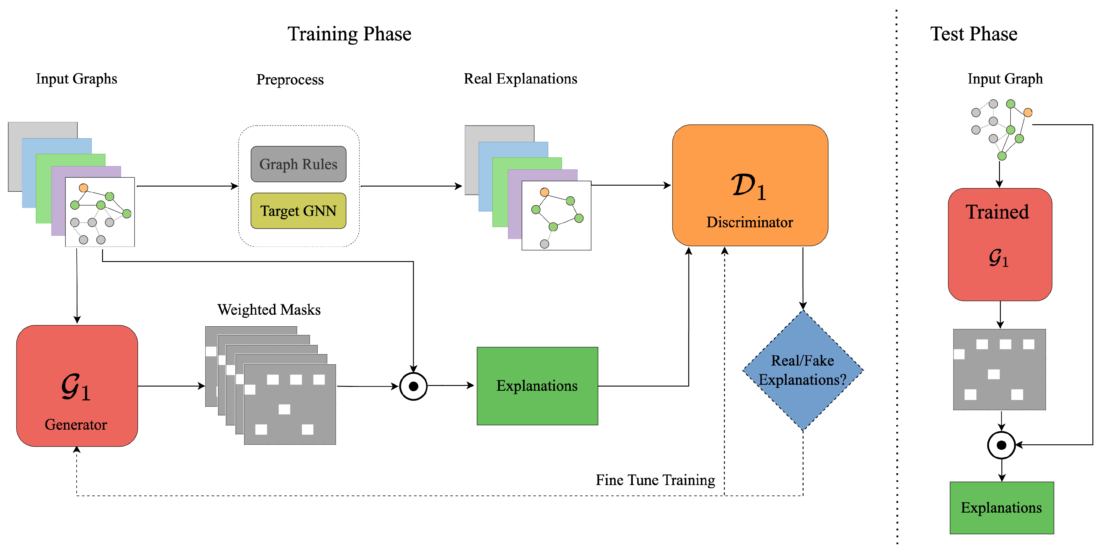
Figure 2.
The framework of ACGAN-GNNExplainer. The symbol ⊙ denotes element-wise multiplication. The framework consists of two phases: the Training Phase and the Testing Phase. During the Training Phase, both the generator and discriminator of the ACGAN-GNNExplainer model are trained. Once training is complete, the Testing Phase uses the trained generator to produce explanations for the test data.
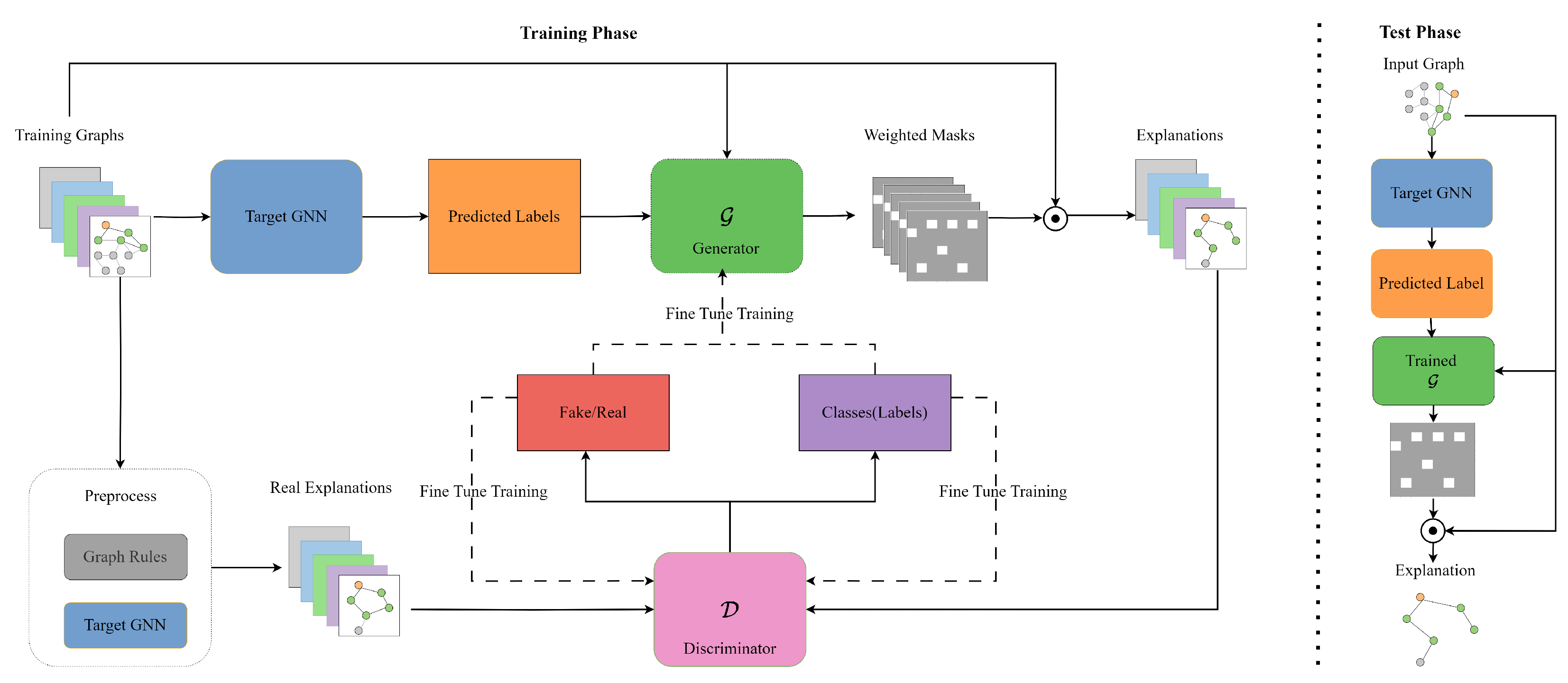

Table 1.
Details of synthetic and real-world datasets.
| Node Classification | Graph Classification | |||
|---|---|---|---|---|
| BA-Shapes | Tree-Cycles | Mutagenicity | NCI1 | |
| # of Graphs | 1 | 1 | 4,337 | 4110 |
| # of Edges | 4110 | 1950 | 266,894 | 132,753 |
| # of Nodes | 700 | 871 | 131,488 | 122,747 |
| # of Labels | 4 | 2 | 2 | 2 |
Table 2.
Explanation accuracy on the BA-Shapes dataset. The presented outcomes encompass averages from five runs alongside their corresponding standard deviations. Notably, the best-performing results have been emphasised in bold.
Table 2.
Explanation accuracy on the BA-Shapes dataset. The presented outcomes encompass averages from five runs alongside their corresponding standard deviations. Notably, the best-performing results have been emphasised in bold.
| K (edges) | 5 | 6 | 7 | 8 | 9 |
| GNNExplainer | 0.7941 | 0.8824 | 0.9118 | 0.9118 | 0.9118 |
| Gem | 0.9412 | 0.9412 | 0.9412 | 0.9412 | 0.9412 |
| GAN-GNNExplainer | 0.6764 | 0.9706 | 0.9706 | 0.9706 | 0.9412 |
Table 3.
Explanation accuracy on the Tree-Cycles dataset. The presented outcomes encompass averages from five runs alongside their corresponding standard deviations. Notably, the best-performing results have been emphasised in bold.
Table 3.
Explanation accuracy on the Tree-Cycles dataset. The presented outcomes encompass averages from five runs alongside their corresponding standard deviations. Notably, the best-performing results have been emphasised in bold.
| K (edges) | 6 | 7 | 8 | 9 | 10 |
| GNNExplainer | 0.2000 | 0.5429 | 0.7143 | 0.8571 | 0.9429 |
| Gem | 0.7142 | 0.8285 | 0.5714 | 0.8285 | 0.9428 |
| GAN-GNNExplainer | 0.9429 | 0.9715 | 0.9429 | 1.0000 | 1.0000 |
Table 4.
Explanation accuracy on the Mutagenicity dataset. The presented outcomes encompass averages from five runs alongside their corresponding standard deviations. Notably, the best-performing results have been emphasised in bold.
Table 4.
Explanation accuracy on the Mutagenicity dataset. The presented outcomes encompass averages from five runs alongside their corresponding standard deviations. Notably, the best-performing results have been emphasised in bold.
| R (edge ratio) | 0.5 | 0.6 | 0.7 | 0.8 | 0.9 |
| GNNExplainer | 0.6175 | 0.5968 | 0.6313 | 0.6935 | 0.7811 |
| Gem | 0.5737 | 0.6014 | 0.6590 | 0.7235 | 0.7903 |
| GAN-GNNExplainer | 0.5914 | 0.5956 | 0.6929 | 0.7215 | 0.7598 |
Table 5.
Explanation accuracy on the NCI1 dataset. The presented outcomes encompass averages from five runs alongside their corresponding standard deviations. Notably, the best-performing results have been emphasised in bold.
Table 5.
Explanation accuracy on the NCI1 dataset. The presented outcomes encompass averages from five runs alongside their corresponding standard deviations. Notably, the best-performing results have been emphasised in bold.
| R (edge ratio) | 0.5 | 0.6 | 0.7 | 0.8 | 0.9 |
| GNNExplainer | 0.5961 | 0.6107 | 0.6788 | 0.7616 | 0.8127 |
| Gem | 0.5645 | 0.6083 | 0.6837 | 0.7518 | 0.8321 |
| GAN-GNNExplainer | 0.6375 | 0.6496 | 0.7105 | 0.7616 | 0.7762 |
Table 6.
The results of explanations on BA-Shapes dataset: , , . The presented outcomes encompass averages from five runs alongside their corresponding standard deviations. Notably, the best-performing results have been emphasised in bold. In this table, refers to our proposed method ACGAN-GNNExplainer.
| K | Metrics | GNNExplainer | Gem | OrphicX | |
| 5 | 0.7941 | 0.9412 | 0.7353 | 0.7941 | |
| 0.7059 | 0.5588 | 0.7941 | 0.6471 | ||
| 0.1471 | 0.000 | 0.2059 | 0.1471 | ||
| 6 | 0.8824 | 0.9706 | 0.7353 | 0.8529 | |
| 0.6765 | 0.5588 | 0.7941 | 0.5882 | ||
| 0.0588 | -0.0294 | 0.2059 | 0.0882 | ||
| 7 | 0.9118 | 0.9706 | 0.8529 | 0.9706 | |
| 0.7059 | 0.5882 | 0.7941 | 0.6176 | ||
| 0.0294 | -0.0294 | 0.0882 | -0.0294 | ||
| 8 | 0.9412 | 0.9706 | 0.8824 | 0.9706 | |
| 0.7353 | 0.5882 | 0.7941 | 0.6471 | ||
| 0.000 | -0.0294 | 0.0588 | -0.0294 | ||
| 9 | 0.9118 | 0.9706 | 0.8824 | 1.000 | |
| 0.7353 | 0.5882 | 0.7941 | 0.6471 | ||
| 0.0294 | -0.0294 | 0.0588 | -0.0588 |
Table 7.
The results of explanations on Tree-Cycles dataset: , , . The presented outcomes encompass averages from five runs alongside their corresponding standard deviations. Notably, the best-performing results have been emphasised in bold. In this table, refers to our proposed method ACGAN-GNNExplainer.
| K | Metrics | GNNExplainer | Gem | OrphicX | |
| 6 | 0.1714 | 0.7143 | 0.9714 | 0.9714 | |
| 0.9143 | 0.9714 | 0.9429 | 0.9714 | ||
| 0.8000 | 0.2571 | 0.0000 | 0.0000 | ||
| 7 | 0.5143 | 0.8286 | 0.9714 | 1.0000 | |
| 0.9429 | 0.9714 | 0.9429 | 0.9714 | ||
| 0.4571 | 0.1429 | 0.0000 | 0.0286 | ||
| 8 | 0.8000 | 0.7143 | 1.0000 | 0.9429 | |
| 0.9714 | 0.9714 | 0.9429 | 0.9714 | ||
| 0.1714 | 0.2571 | 0.0286 | 0.0286 | ||
| 9 | 0.9143 | 0.8571 | 1.0000 | 0.9143 | |
| 0.9714 | 0.9714 | 0.9429 | 0.9714 | ||
| 0.0571 | 0.1143 | 0.0286 | 0.0571 | ||
| 10 | 0.9143 | 0.8857 | 1.0000 | 0.9714 | |
| 0.9714 | 0.9714 | 0.9429 | 0.9714 | ||
| 0.0571 | 0.0857 | 0.0286 | 0.0000 |
Table 8.
The results of explanations on Mutagenicity dataset: , , . The presented outcomes encompass averages from five runs alongside their corresponding standard deviations. Notably, the best-performing results have been emphasised in bold. In this table, refers to our proposed method ACGAN-GNNExplainer.
| R | Metrics | GNNExplainer | Gem | OrphicX | |
| 0.5 | 0.6175 | 0.5737 | 0.4539 | 0.6175 | |
| 0.3618 | 0.3018 | 0.2419 | 0.3963 | ||
| 0.2535 | 0.2972 | 0.4171 | 0.2535 | ||
| 0.6 | 0.5968 | 0.6014 | 0.5599 | 0.6037 | |
| 0.3825 | 0.3295 | 0.2949 | 0.3828 | ||
| 0.2742 | 0.2696 | 0.3111 | 0.2673 | ||
| 0.7 | 0.6313 | 0.659 | 0.6244 | 0.7074 | |
| 0.3963 | 0.2857 | 0.2995 | 0.3986 | ||
| 0.2396 | 0.212 | 0.2465 | 0.1636 | ||
| 0.8 | 0.6935 | 0.7235 | 0.7097 | 0.7673 | |
| 0.3641 | 0.2581 | 0.3157 | 0.3602 | ||
| 0.1774 | 0.1475 | 0.1613 | 0.1037 | ||
| 0.9 | 0.7811 | 0.7903 | 0.8111 | 0.7903 | |
| 0.3641 | 0.212 | 0.2949 | 0.3871 | ||
| 0.0899 | 0.0806 | 0.0599 | 0.0806 |
Table 9.
The results of explanations on NCI1 dataset: , , . The presented outcomes encompass averages from five runs alongside their corresponding standard deviations. Notably, the best-performing results have been emphasised in bold. In this table, refers to our proposed method ACGAN-GNNExplainer.
Table 9.
The results of explanations on NCI1 dataset: , , . The presented outcomes encompass averages from five runs alongside their corresponding standard deviations. Notably, the best-performing results have been emphasised in bold. In this table, refers to our proposed method ACGAN-GNNExplainer.
| R | Metrics | GNNExplainer | Gem | OrphicX | |
| 0.5 | 0.5961 | 0.5645 | 0.562 | 0.6569 | |
| 0.3358 | 0.3796 | 0.3114 | 0.4015 | ||
| 0.2749 | 0.3066 | 0.309 | 0.2141 | ||
| 0.6 | 0.6107 | 0.6083 | 0.6496 | 0.6496 | |
| 0.3625 | 0.4307 | 0.3431 | 0.4523 | ||
| 0.2603 | 0.2628 | 0.3236 | 0.2214 | ||
| 0.7 | 0.6788 | 0.6837 | 0.6083 | 0.6861 | |
| 0.3844 | 0.4282 | 0.3382 | 0.4453 | ||
| 0.1922 | 0.1873 | 0.2628 | 0.1849 | ||
| 0.8 | 0.7616 | 0.7518 | 0.708 | 0.7932 | |
| 0.3747 | 0.4404 | 0.3698 | 0.4672 | ||
| 0.1095 | 0.1192 | 0.163 | 0.0779 | ||
| 0.9 | 0.8127 | 0.8321 | 0.8102 | 0.8446 | |
| 0.3236 | 0.3212 | 0.3139 | 0.3942 | ||
| 0.0584 | 0.0389 | 0.0608 | 0.0254 |
Disclaimer/Publisher’s Note: The statements, opinions and data contained in all publications are solely those of the individual author(s) and contributor(s) and not of MDPI and/or the editor(s). MDPI and/or the editor(s) disclaim responsibility for any injury to people or property resulting from any ideas, methods, instructions or products referred to in the content. |
© 2024 by the authors. Licensee MDPI, Basel, Switzerland. This article is an open access article distributed under the terms and conditions of the Creative Commons Attribution (CC BY) license (http://creativecommons.org/licenses/by/4.0/).
Copyright: This open access article is published under a Creative Commons CC BY 4.0 license, which permit the free download, distribution, and reuse, provided that the author and preprint are cited in any reuse.


