Submitted:
24 October 2024
Posted:
25 October 2024
You are already at the latest version
Abstract
Keywords:
1. Introduction
2. Related work
3. Materials and Methods
3.1. GIGAScience Dataset for MI-EEG
3.2. Subject-Dependent MI-EEG Classification Using Deep Learning
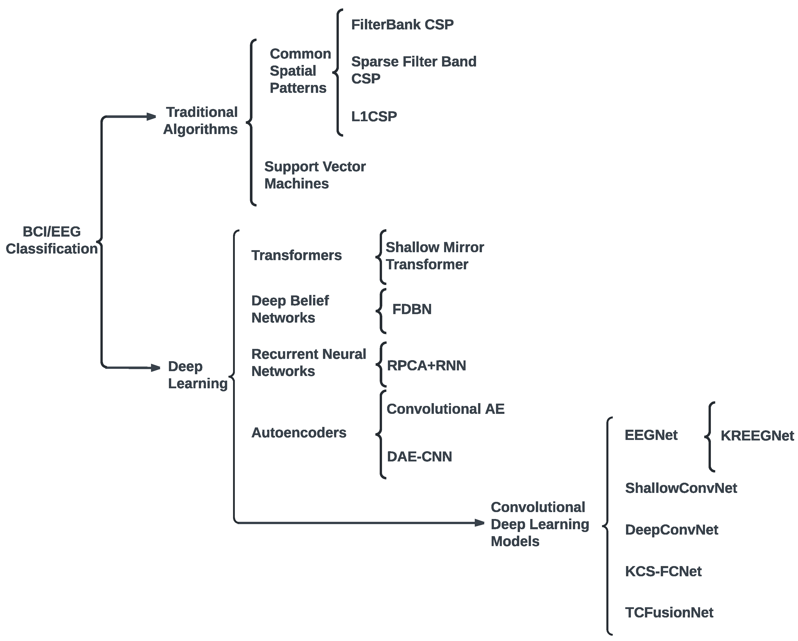
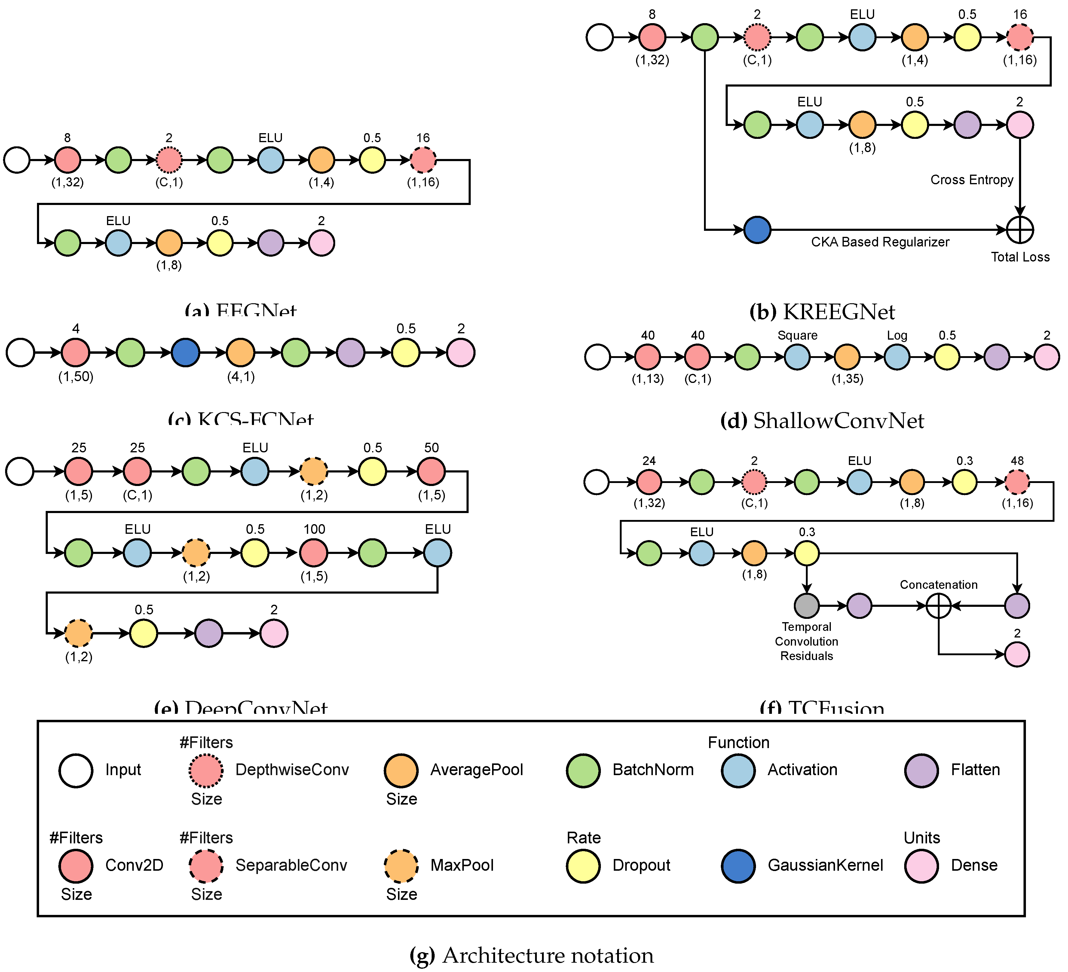
- EEGNet [36]: The process begins with a temporal convolution, which is followed by a depthwise layer that serves as a spatial representation for each filter produced at the previous stage. Afterward, an exponential linear activation function (ELU) is used before an average pooling and a dropout to help minimize overfitting. Next, it applies a separable convolution, which is followed by another ELU activation and an average pooling. Lastly, a second dropout layer precedes the flattening and classification stages. Batch normalization is always performed immediately after each convolutional layer.
- KREEGNet [38]: Similar to EEGNet, it uses a Gaussian kernel after batch normalization to extract the connectivity between EEG channels. A delta kernel is implemented on the label data, and a Centered Kernel Alignment (CKA)-based regularization between connectivities and label data is added as a penalty to the straightforward cross-entropy.
- KCS-FCNet [39]: A single convolutional stage before using a gaussian kernel to measure EEG connectivity is utilized. These are then run through an average pooling layer before batch normalization and classification. Interestingly enough, a dropout step is done between the flatten layer and the dense layer.
- ShallowConvNet [61]: It performs two consecutive convolutions, then proceeds with batch normalization and square activation. After that, average pooling is done before logarithmic activation and dropout. Finally, a layer of flattening and density is applied for classification.
- DeepConvNet [19]: The system employs two convolutional layers sequentially, followed by batch normalization and ELU activation. Then, a max pooling and a dropout are employed before another convolutional layer and batch normalization. Another set of ELU activation, max pooling, and dropouts is performed before a final convolution and batch normalization. Finally, another ELU, max pooling, and dropout are performed before classifying.
- TCFusionNet [37]: Similar to EEGNet, it employs a sequence of residual blocks to gather extra data prior to classification. Each residual block is comprised of a dilated convolution followed by batch normalization, ELU, and dropout twice. In parallel, a 1x1 convolution is done and then concatenated to the output of the residual block. Before flattening and joining the flattened features from the separable convolution stage, multiple residual blocks are put in place in a cascading fashion. Finally, a dense layer is used for classification.
3.3. Layer-Wise Class Activation Maps for Explainable MI-EEG Classification
3.4. Questionnaire-MI Performance Canonical Correlation Analysis (QMIP-CCA)
3.5. Multimodal and Explainable Deep Learning Implementation Details
4. Results and Discussion
4.1. MI Classification Performance
4.2. Explainable MI-EEG Classification Results
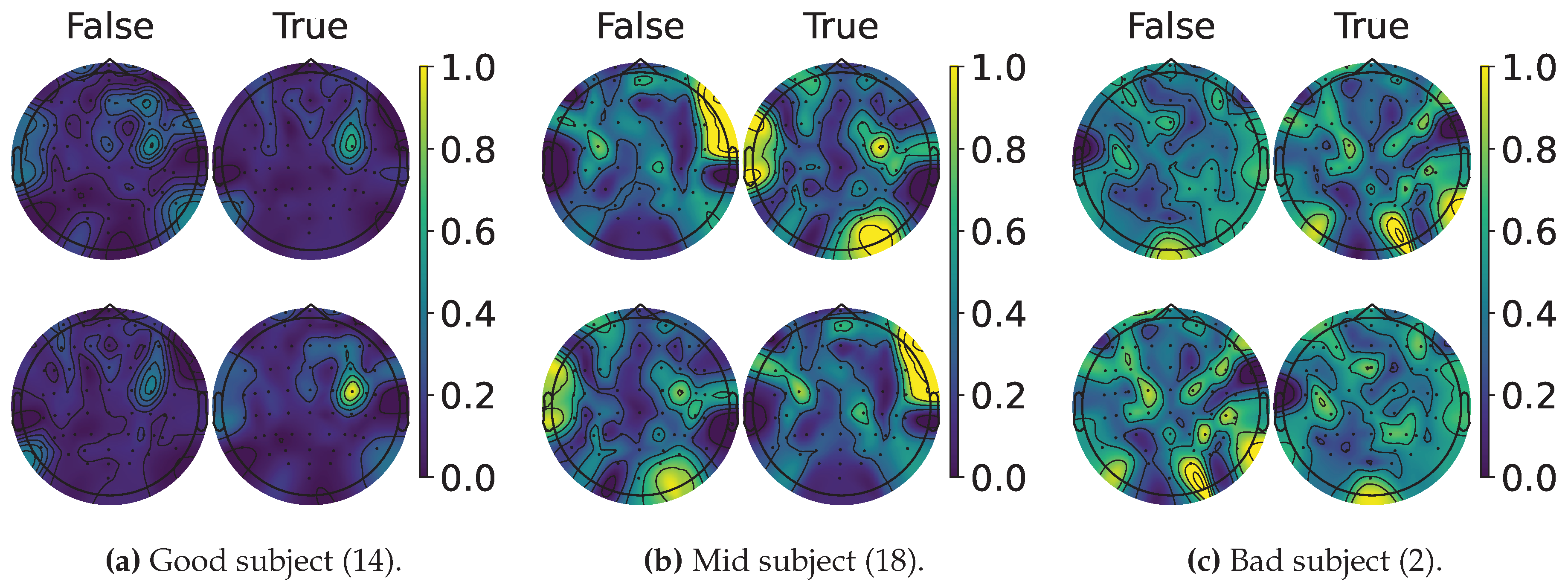
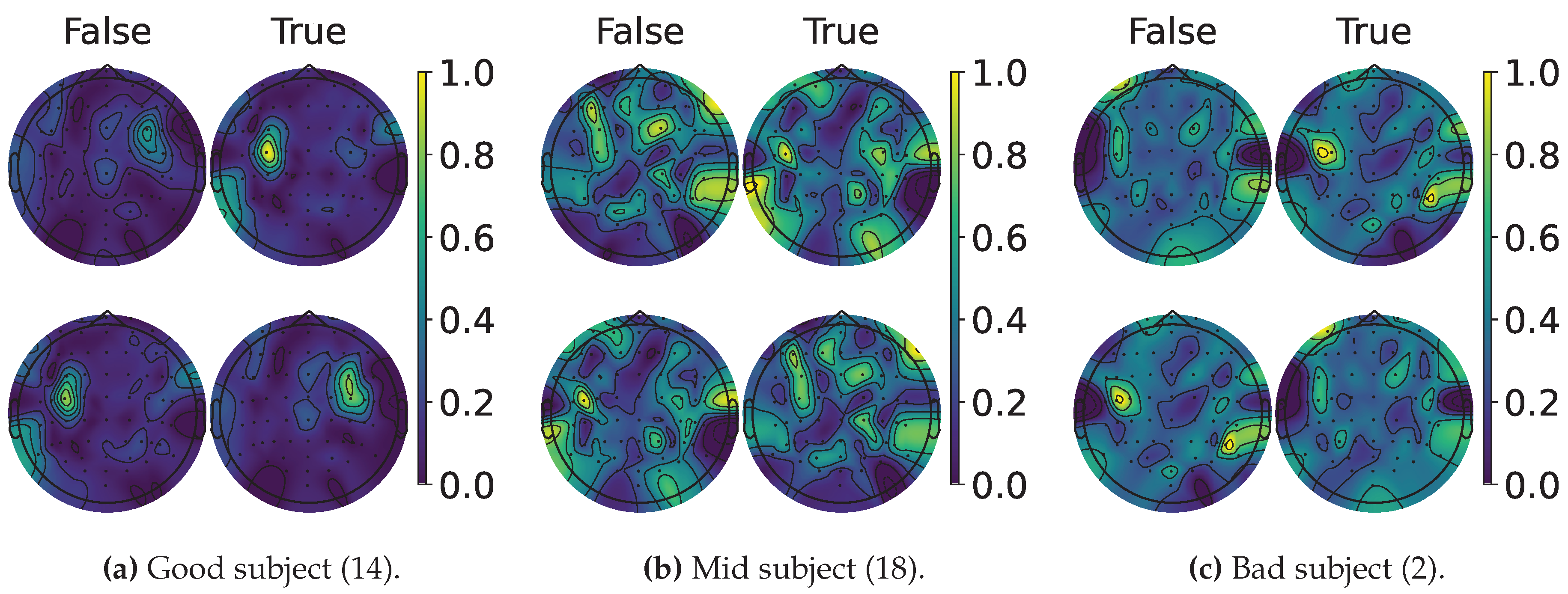
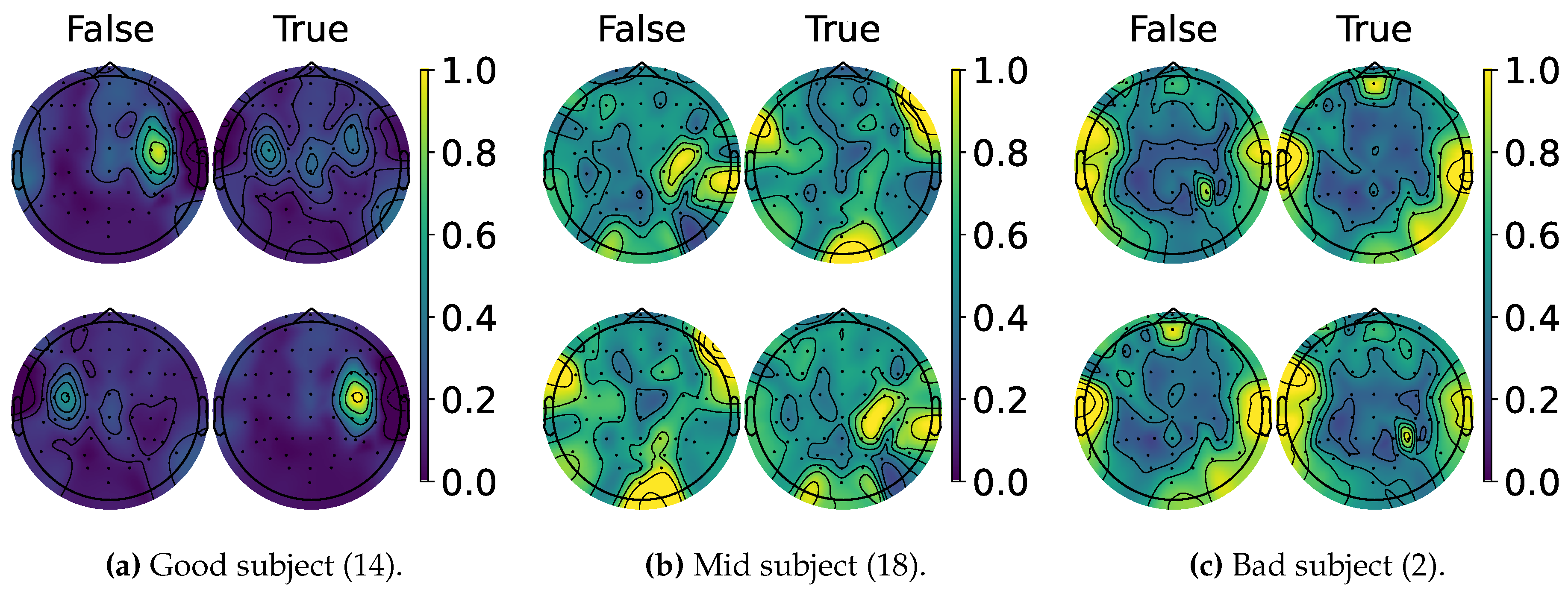
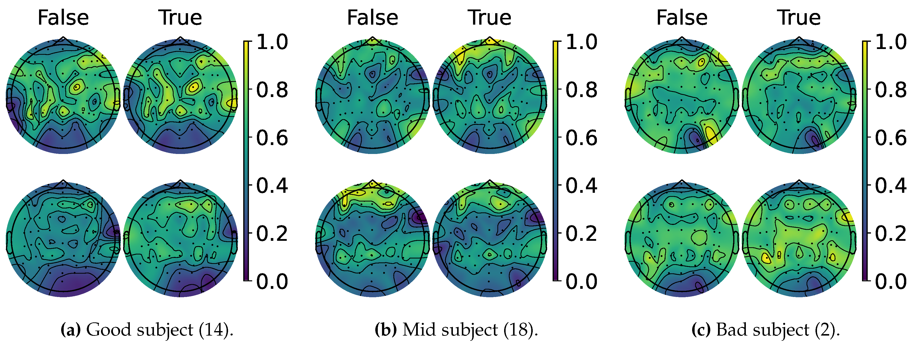
4.3. Questionnaire and MI-EEG Performance Relevance Analysis Results
5. Conclusions
Author Contributions
Funding
Institutional Review Board Statement
Informed Consent Statement
Data Availability Statement
Conflicts of Interest
Appendix A. Additional Results
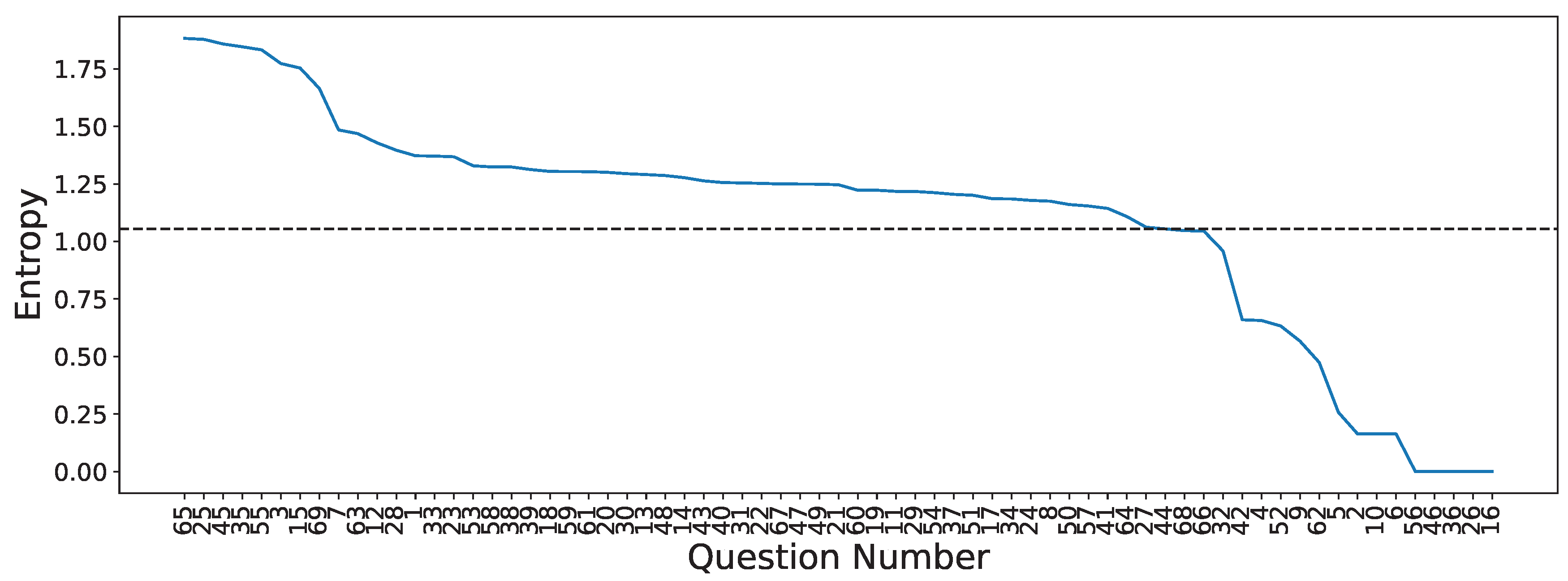
| Set | Question | Answer Type | Entropy |
|---|---|---|---|
| Pre-MI | Time slot | (1=9:30/2=12:30/3=15:30/4=19:00) | 1.373 |
| Age | (number) | 1.774 | |
| How long did you sleep? | (1=less than 4h/2=5 6h/3=6 7h/4=7 8/5=more than 8) | 1.485 | |
| Did you drink coffee within the past 24 hours | (0=no, number=hours before) | 1.172 | |
| How do you feel? | Relaxed 1 2 3 4 5 Anxious | 1.218 | |
| How do you feel? | Exciting 1 2 3 4 5 Boring | 1.429 | |
| How do you feel? | Very good 1 2 3 4 5 Very bad or tired | 1.291 | |
| How do you feel? | Very good 1 2 3 4 5 Very bad or tired | 1.277 | |
| The BCI performance (accuracy) expected? | % | 1.754 | |
| Run 1 | How do you feel? | Relaxed 1 2 3 4 5 Anxious | 1.186 |
| How do you feel? | Exciting 1 2 3 4 5 Boring | 1.305 | |
| How do you feel? | High 1 2 3 4 5 Low | 1.223 | |
| How do you feel? | Very good 1 2 3 4 5 Very bad or tired | 1.301 | |
| How do you feel? | Very good 1 2 3 4 5 Very bad or tired | 1.247 | |
| Have you nodded off (slept a while) during this run? | (0=no/number = how many times) | 1.253 | |
| Was it easy to imagine finger movements? | Easy 1 2 3 4 5 Difficult | 1.368 | |
| How many trials you missed? | (0=no/number = how many times) | 1.179 | |
| The BCI performance (accuracy) expected? | % | 1.879 | |
| Run 2 | How do you feel? | Relaxed 1 2 3 4 5 Anxious | 1.062 |
| How do you feel? | Exciting 1 2 3 4 5 Boring | 1.397 | |
| How do you feel? | High 1 2 3 4 5 Low | 1.217 | |
| How do you feel? | Very good 1 2 3 4 5 Very bad or tired | 1.295 | |
| How do you feel? | Very good 1 2 3 4 5 Very bad or tired | 1.254 | |
| Was it easy to imagine finger movements? | Easy 1 2 3 4 5 Difficult | 1.371 | |
| How many trials you missed? | (0=no/number = how many times) | 1.185 | |
| The BCI performance (accuracy) expected? | % | 1.846 | |
| Run 3 | How do you feel? | Relaxed 1 2 3 4 5 Anxious | 1.205 |
| How do you feel? | Exciting 1 2 3 4 5 Boring | 1.324 | |
| How do you feel? | High 1 2 3 4 5 Low | 1.313 | |
| How do you feel? | Very good 1 2 3 4 5 Very bad or tired | 1.256 | |
| How do you feel? | Very good 1 2 3 4 5 Very bad or tired | 1.144 | |
| Was it easy to imagine finger movements? | Easy 1 2 3 4 5 Difficult | 1.263 | |
| How many trials you missed? | (0=no/number = how many times) | 1.055 | |
| The BCI performance (accuracy) expected? | % | 1.859 | |
| Run 4 | How do you feel? | Relaxed 1 2 3 4 5 Anxious | 1.250 |
| How do you feel? | Exciting 1 2 3 4 5 Boring | 1.287 | |
| How do you feel? | High 1 2 3 4 5 Low | 1.249 | |
| How do you feel? | Very good 1 2 3 4 5 Very bad or tired | 1.161 | |
| How do you feel? | Very good 1 2 3 4 5 Very bad or tired | 1.201 | |
| Was it easy to imagine finger movements? | Easy 1 2 3 4 5 Difficult | 1.329 | |
| How many trials you missed? | (0=no/number = how many times) | 1.212 | |
| The BCI performance (accuracy) expected? | % | 1.833 | |
| Run 5 | How do you feel? | Relaxed 1 2 3 4 5 Anxious | 1.154 |
| How do you feel? | Exciting 1 2 3 4 5 Boring | 1.324 | |
| How do you feel? | High 1 2 3 4 5 Low | 1.304 | |
| How do you feel? | Very good 1 2 3 4 5 Very bad or tired | 1.223 | |
| How do you feel? | Very good 1 2 3 4 5 Very bad or tired | 1.304 | |
| Was it easy to imagine finger movements? | Easy 1 2 3 4 5 Difficult | 1.469 | |
| How many trials you missed? | (0=no/number = how many times) | 1.108 | |
| The BCI performance (accuracy) expected? | % | 1.883 | |
| Post-MI | How was this experiment? | Good 1 2 3 4 5 Bad | 1.250 |
| The BCI performance (accuracy) of whole data expected? | % | 1.665 |
References
- Unesco.; for Engineering Education, U.I.C.; she, Z.y.b.y.c.b. Engineering for sustainable development : delivering on the Sustainable Development Goals; United Nations Educational, Scientific, and Cultural Organization ; International Center for Engineering Education under the auspices of UNESCO : Compilation and Translation Press: Paris, France, Beijing, China, 2021.
- Mayo Clinic Editorial Staff. EEG (electroencephalogram). https://www.mayoclinic.org/tests-procedures/eeg/about/pac-20393875, 2024.
- Altaheri, H.; Muhammad, G.; Alsulaiman, M.; Amin, S.U.; Altuwaijri, G.A.; Abdul, W.; Bencherif, M.A.; Faisal, M. Deep learning techniques for classification of electroencephalogram (EEG) motor imagery (MI) signals: A review. Neural Computing and Applications 2023, 35, 14681–14722. [Google Scholar] [CrossRef]
- Ramadan, R.A.; Altamimi, A.B. Unraveling the potential of brain-computer interface technology in medical diagnostics and rehabilitation: A comprehensive literature review. Health and Technology 2024, 14, 263–276. [Google Scholar] [CrossRef]
- Abidi, M.; De Marco, G.; Grami, F.; Termoz, N.; Couillandre, A.; Querin, G.; Bede, P.; Pradat, P.F. Neural correlates of motor imagery of gait in amyotrophic lateral sclerosis. Journal of Magnetic Resonance Imaging 2021, 53, 223–233. [Google Scholar] [CrossRef] [PubMed]
- Zhang, H.; Zhao, M.; Wei, C.; Mantini, D.; Li, Z.; Liu, Q. EEGdenoiseNet: a benchmark dataset for deep learning solutions of EEG denoising. Journal of Neural Engineering 2021, 18, 056057. [Google Scholar] [CrossRef] [PubMed]
- Saini, M.; Satija, U.; Upadhayay, M.D. Wavelet based waveform distortion measures for assessment of denoised EEG quality with reference to noise-free EEG signal. IEEE Signal Processing Letters 2020, 27, 1260–1264. [Google Scholar] [CrossRef]
- Tsuchimoto, S.; Shibusawa, S.; Iwama, S.; Hayashi, M.; Okuyama, K.; Mizuguchi, N.; Kato, K.; Ushiba, J. Use of common average reference and large-Laplacian spatial-filters enhances EEG signal-to-noise ratios in intrinsic sensorimotor activity. Journal of neuroscience methods 2021, 353, 109089. [Google Scholar] [CrossRef] [PubMed]
- Croce, P.; Quercia, A.; Costa, S.; Zappasodi, F. EEG microstates associated with intra-and inter-subject alpha variability. Scientific reports 2020, 10, 2469. [Google Scholar] [CrossRef] [PubMed]
- Saha, S.; Baumert, M. Intra-and inter-subject variability in EEG-based sensorimotor brain computer interface: a review. Frontiers in computational neuroscience 2020, 13, 87. [Google Scholar] [CrossRef]
- Maswanganyi, R.C.; Tu, C.; Owolawi, P.A.; Du, S. Statistical evaluation of factors influencing inter-session and inter-subject variability in eeg-based brain computer interface. IEEE Access 2022, 10, 96821–96839. [Google Scholar] [CrossRef]
- Blanco-Diaz, C.F.; Antelis, J.M.; Ruiz-Olaya, A.F. Comparative analysis of spectral and temporal combinations in CSP-based methods for decoding hand motor imagery tasks. Journal of Neuroscience Methods 2022, 371, 109495. [Google Scholar] [CrossRef]
- Wang, B.; Wong, C.M.; Kang, Z.; Liu, F.; Shui, C.; Wan, F.; Chen, C.P. Common spatial pattern reformulated for regularizations in brain–computer interfaces. IEEE transactions on cybernetics 2020, 51, 5008–5020. [Google Scholar] [CrossRef]
- Galindo-Noreña, S.; Cárdenas-Peña, D.; Orozco-Gutierrez, A. Multiple Kernel Stein Spatial Patterns for the Multiclass Discrimination of Motor Imagery Tasks. Applied Sciences 2020, 10. [Google Scholar] [CrossRef]
- Geng, X.; Li, D.; Chen, H.; Yu, P.; Yan, H.; Yue, M. An improved feature extraction algorithms of EEG signals based on motor imagery brain-computer interface. Alexandria Engineering Journal 2022, 61, 4807–4820. [Google Scholar] [CrossRef]
- Chollet, F. Deep Learning with Python; Manning, 2017.
- Collazos-Huertas, D.F.; Álvarez-Meza, A.M.; Castellanos-Dominguez, G. Image-based learning using gradient class activation maps for enhanced physiological interpretability of motor imagery skills. Applied Sciences 2022, 12, 1695. [Google Scholar] [CrossRef]
- Rakhmatulin, I.; Dao, M.S.; Nassibi, A.; Mandic, D. Exploring Convolutional Neural Network Architectures for EEG Feature Extraction. Sensors 2024, 24. [Google Scholar] [CrossRef] [PubMed]
- Schirrmeister, R.T.; Springenberg, J.T.; Fiederer, L.D.J.; Glasstetter, M.; Eggensperger, K.; Tangermann, M.; Hutter, F.; Burgard, W.; Ball, T. Deep learning with convolutional neural networks for EEG decoding and visualization. Human Brain Mapping 2017, 38, 5391–5420. [Google Scholar] [CrossRef] [PubMed]
- Li, F.; He, F.; Wang, F.; Zhang, D.; Xia, Y.; Li, X. A novel simplified convolutional neural network classification algorithm of motor imagery EEG signals based on deep learning. Applied Sciences 2020, 10, 1605. [Google Scholar] [CrossRef]
- Liu, J.; Wu, G.; Luo, Y.; Qiu, S.; Yang, S.; Li, W.; Bi, Y. EEG-based emotion classification using a deep neural network and sparse autoencoder. Frontiers in Systems Neuroscience 2020, 14, 43. [Google Scholar] [CrossRef] [PubMed]
- Chowdary, M.K.; Anitha, J.; Hemanth, D.J. Emotion recognition from EEG signals using recurrent neural networks. Electronics 2022, 11, 2387. [Google Scholar] [CrossRef]
- Ma, Y.; Song, Y.; Gao, F. A novel hybrid CNN-transformer model for EEG motor imagery classification. In Proceedings of the 2022 International Joint Conference on Neural Networks (IJCNN); IEEE, 2022; pp. 1–8. [Google Scholar]
- Li, X.; Xiong, H.; Li, X.; Wu, X.; Zhang, X.; Liu, J.; Bian, J.; Dou, D. Interpretable deep learning: Interpretation, interpretability, trustworthiness, and beyond. Knowledge and Information Systems 2022, 64, 3197–3234. [Google Scholar] [CrossRef]
- Bhardwaj, H.; Tomar, P.; Sakalle, A.; Ibrahim, W. Eeg-based personality prediction using fast fourier transform and deeplstm model. Computational Intelligence and Neuroscience 2021, 2021, 6524858. [Google Scholar] [CrossRef] [PubMed]
- Cho, H.; Ahn, M.; Ahn, S.; Kwon, M.; Jun, S.C. EEG datasets for motor imagery brain–computer interface. GigaScience 2017, 6, gix034. [Google Scholar] [CrossRef] [PubMed]
- Rahman, A.U.; Tubaishat, A.; Al-Obeidat, F.; Halim, Z.; Tahir, M.; Qayum, F. Extended ICA and M-CSP with BiLSTM towards improved classification of EEG signals. Soft Computing 2022, 26, 10687–10698. [Google Scholar] [CrossRef]
- Jin, J.; Xiao, R.; Daly, I.; Miao, Y.; Wang, X.; Cichocki, A. Internal Feature Selection Method of CSP Based on L1-Norm and Dempster–Shafer Theory. IEEE Transactions on Neural Networks and Learning Systems 2021, 32, 4814–4825. [Google Scholar] [CrossRef] [PubMed]
- Wang, H.; Tang, Q.; Zheng, W. L1-Norm-Based Common Spatial Patterns. IEEE Transactions on Biomedical Engineering 2012, 59, 653–662. [Google Scholar] [CrossRef] [PubMed]
- Ang, K.K.; Chin, Z.Y.; Zhang, H.; Guan, C. Filter Bank Common Spatial Pattern (FBCSP) in Brain-Computer Interface. In Proceedings of the 2008 IEEE International Joint Conference on Neural Networks (IEEE World Congress on Computational Intelligence); 2008; pp. 2390–2397. [Google Scholar] [CrossRef]
- Zhang, Y.; Zhou, G.; Jin, J.; Wang, X.; Cichocki, A. Optimizing spatial patterns with sparse filter bands for motor-imagery based brain–computer interface. Journal of neuroscience methods 2015, 255, 85–91. [Google Scholar] [CrossRef] [PubMed]
- Miao, Y.; Jin, J.; Daly, I.; Zuo, C.; Wang, X.; Cichocki, A.; Jung, T.P. Learning common time-frequency-spatial patterns for motor imagery classification. IEEE Transactions on Neural Systems and Rehabilitation Engineering 2021, 29, 699–707. [Google Scholar] [CrossRef]
- Luo, J.; Gao, X.; Zhu, X.; Wang, B.; Lu, N.; Wang, J. Motor imagery EEG classification based on ensemble support vector learning. Computer methods and programs in biomedicine 2020, 193, 105464. [Google Scholar] [CrossRef] [PubMed]
- Tibrewal, N.; Leeuwis, N.; Alimardani, M. Classification of motor imagery EEG using deep learning increases performance in inefficient BCI users. Plos one 2022, 17, e0268880. [Google Scholar] [CrossRef]
- Lopes, M.; Cassani, R.; Falk, T.H. Using CNN Saliency Maps and EEG Modulation Spectra for Improved and More Interpretable Machine Learning-Based Alzheimer’s Disease Diagnosis. Computational Intelligence and Neuroscience 2023, 2023, 3198066. [Google Scholar] [CrossRef] [PubMed]
- Lawhern, V.J.; Solon, A.J.; Waytowich, N.R.; Gordon, S.M.; Hung, C.P.; Lance, B.J. EEGNet: a compact convolutional neural network for EEG-based brain–computer interfaces. Journal of Neural Engineering 2018, 15, 056013. [Google Scholar] [CrossRef] [PubMed]
- Musallam, Y.K.; AlFassam, N.I.; Muhammad, G.; Amin, S.U.; Alsulaiman, M.; Abdul, W.; Altaheri, H.; Bencherif, M.A.; Algabri, M. Electroencephalography-based motor imagery classification using temporal convolutional network fusion. Biomedical Signal Processing and Control 2021, 69, 102826. [Google Scholar] [CrossRef]
- Tobón-Henao, M.; Álvarez Meza, A.M.; Castellanos-Dominguez, C.G. Kernel-Based Regularized EEGNet Using Centered Alignment and Gaussian Connectivity for Motor Imagery Discrimination. Computers 2023, 12. [Google Scholar] [CrossRef]
- García-Murillo, D.G.; Álvarez Meza, A.M.; Castellanos-Dominguez, C.G. KCS-FCnet: Kernel Cross-Spectral Functional Connectivity Network for EEG-Based Motor Imagery Classification. Diagnostics 2023, 13. [Google Scholar] [CrossRef] [PubMed]
- Lu, N.; Li, T.; Ren, X.; Miao, H. A deep learning scheme for motor imagery classification based on restricted Boltzmann machines. IEEE transactions on neural systems and rehabilitation engineering 2016, 25, 566–576. [Google Scholar] [CrossRef]
- Mirzaei, S.; Ghasemi, P. EEG motor imagery classification using dynamic connectivity patterns and convolutional autoencoder. Biomedical Signal Processing and Control 2021, 68, 102584. [Google Scholar] [CrossRef]
- Hwaidi, J.F.; Chen, T.M. Classification of motor imagery EEG signals based on deep autoencoder and convolutional neural network approach. IEEE access 2022, 10, 48071–48081. [Google Scholar] [CrossRef]
- Wei, C.S.; Keller, C.J.; Li, J.; Lin, Y.P.; Nakanishi, M.; Wagner, J.; Wu, W.; Zhang, Y.; Jung, T.P. Inter-and intra-subject variability in brain imaging and decoding, 2021.
- Alessandrini, M.; Biagetti, G.; Crippa, P.; Falaschetti, L.; Luzzi, S.; Turchetti, C. Eeg-based alzheimer’s disease recognition using robust-pca and lstm recurrent neural network. Sensors 2022, 22, 3696. [Google Scholar] [CrossRef] [PubMed]
- Luo, J.; Wang, Y.; Xia, S.; Lu, N.; Ren, X.; Shi, Z.; Hei, X. A shallow mirror transformer for subject-independent motor imagery BCI. Computers in Biology and Medicine 2023, 164, 107254. [Google Scholar] [CrossRef]
- Bang, J.S.; Lee, S.W. Interpretable convolutional neural networks for subject-independent motor imagery classification. In Proceedings of the 2022 10th International Winter Conference on Brain-Computer Interface (BCI); IEEE, 2022; pp. 1–5. [Google Scholar]
- Bejani, M.M.; Ghatee, M. A systematic review on overfitting control in shallow and deep neural networks. Artificial Intelligence Review 2021, 54, 6391–6438. [Google Scholar] [CrossRef]
- Zhang, Y.; Tiňo, P.; Leonardis, A.; Tang, K. A survey on neural network interpretability. IEEE Transactions on Emerging Topics in Computational Intelligence 2021, 5, 726–742. [Google Scholar] [CrossRef]
- Onishi, S.; Nishimura, M.; Fujimura, R.; Hayashi, Y. Why Do Tree Ensemble Approximators Not Outperform the Recursive-Rule eXtraction Algorithm? Machine Learning and Knowledge Extraction 2024, 6, 658–678. [Google Scholar] [CrossRef]
- Hong, Q.; Wang, Y.; Li, H.; Zhao, Y.; Guo, W.; Wang, X. Probing filters to interpret CNN semantic configurations by occlusion. In Proceedings of the Data Science: 7th International Conference of Pioneering Computer Scientists, Engineers and Educators, ICPCSEE 2021, Taiyuan, China, 2021, ,, September 17–20; Proceedings, Part II 7. Springer, 2021; pp. 103–115. [Google Scholar]
- Christoph, M. Interpretable machine learning: A guide for making black box models explainable; Leanpub, 2020.
- Zhou, B.; Khosla, A.; Lapedriza, A.; Oliva, A.; Torralba, A. Learning Deep Features for Discriminative Localization. In Proceedings of the 2016 IEEE Conference on Computer Vision and Pattern Recognition (CVPR); 2016; pp. 2921–2929. [Google Scholar] [CrossRef]
- Selvaraju, R.R.; Cogswell, M.; Das, A.; Vedantam, R.; Parikh, D.; Batra, D. Grad-CAM: Visual Explanations from Deep Networks via Gradient-Based Localization. International Journal of Computer Vision 2019, 128, 336–359. [Google Scholar] [CrossRef]
- Chattopadhay, A.; Sarkar, A.; Howlader, P.; Balasubramanian, V.N. Grad-CAM++: Generalized Gradient-Based Visual Explanations for Deep Convolutional Networks. In Proceedings of the 2018 IEEE Winter Conference on Applications of Computer Vision (WACV); IEEE, 2018. [Google Scholar] [CrossRef]
- Jiang, P.T.; Zhang, C.B.; Hou, Q.; Cheng, M.M.; Wei, Y. Layercam: Exploring hierarchical class activation maps for localization. IEEE Transactions on Image Processing 2021, 30, 5875–5888. [Google Scholar] [CrossRef] [PubMed]
- Bi, J.; Wang, F.; Yan, X.; Ping, J.; Wen, Y. Multi-domain fusion deep graph convolution neural network for EEG emotion recognition. Neural Computing and Applications 2022, 34, 22241–22255. [Google Scholar] [CrossRef]
- Wu, D.; Zhang, J.; Zhao, Q. Multimodal Fused Emotion Recognition About Expression-EEG Interaction and Collaboration Using Deep Learning. IEEE Access 2020, 8, 133180–133189. [Google Scholar] [CrossRef]
- Collazos-Huertas, D.F.; Velasquez-Martinez, L.F.; Perez-Nastar, H.D.; Alvarez-Meza, A.M.; Castellanos-Dominguez, G. Deep and wide transfer learning with kernel matching for pooling data from electroencephalography and psychological questionnaires. Sensors 2021, 21, 5105. [Google Scholar] [CrossRef]
- Abibullaev, B.; Keutayeva, A.; Zollanvari, A. Deep learning in EEG-based BCIs: a comprehensive review of transformer models, advantages, challenges, and applications. IEEE Access 2023. [Google Scholar] [CrossRef]
- Murphy, K.P. Probabilistic machine learning: an introduction; MIT press, 2022.
- Kim, S.J.; Lee, D.H.; Lee, S.W. Rethinking CNN Architecture for Enhancing Decoding Performance of Motor Imagery-based EEG Signals. IEEE Access 2022. [Google Scholar] [CrossRef]
- Jung, H.; Oh, Y. Towards better explanations of class activation mapping. In Proceedings of the Proceedings of the IEEE/CVF international conference on computer vision, 2021, pp. 1336–1344.
- Fukumizu, K.; Bach, F.R.; Gretton, A. Statistical consistency of kernel canonical correlation analysis. Journal of Machine Learning Research 2007, 8. [Google Scholar]
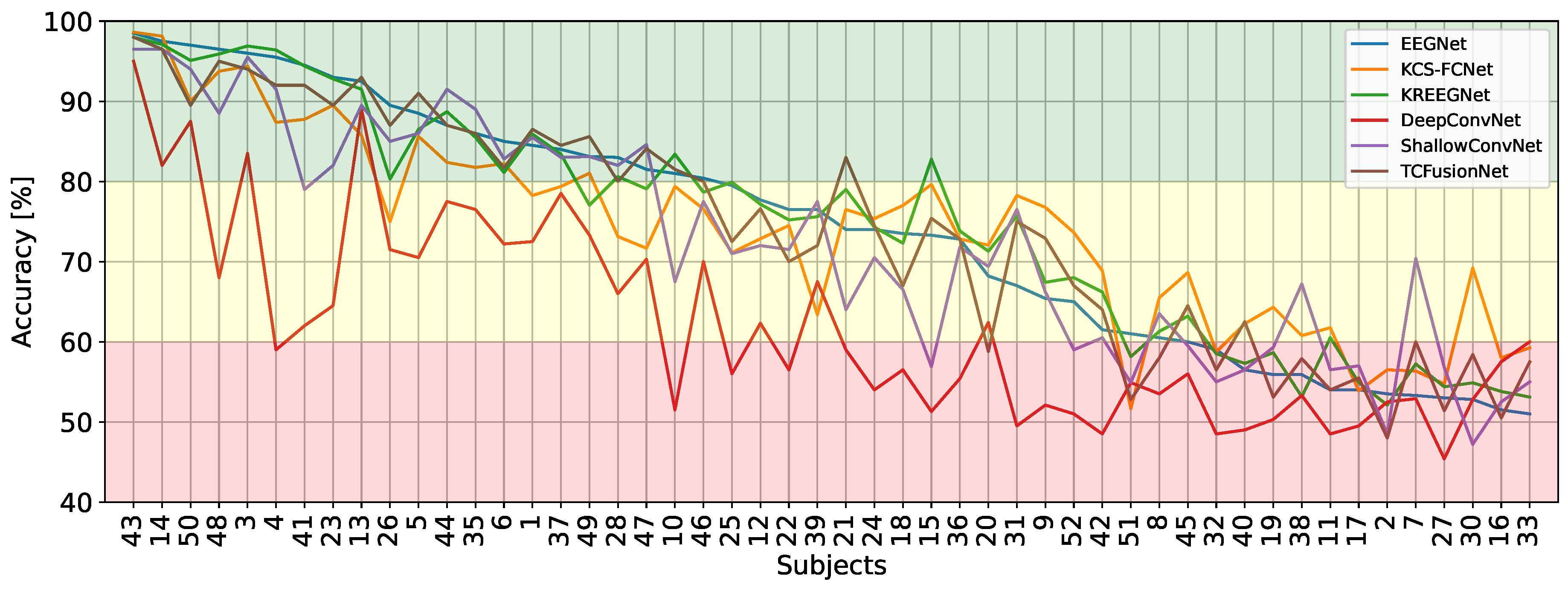


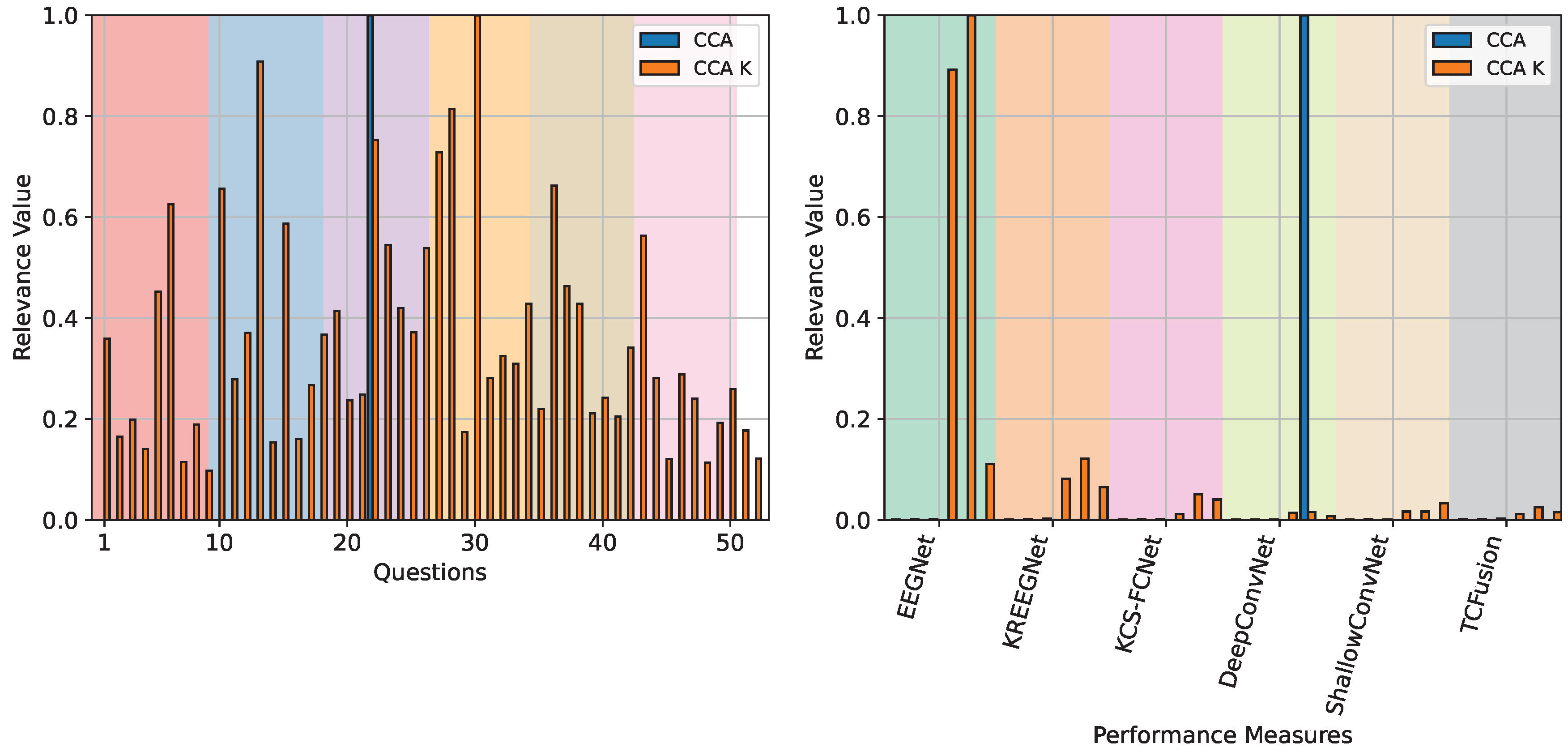
| Training Hyperparameter | Argument | Value |
|---|---|---|
| Monitor | Training Loss | |
| Factor | 0.1 | |
| Reduce learning rate on plateau | Patience | 30 |
| Min Delta | 0.01 | |
| Min Learning Rate | 0 | |
| Adam | Learning Rate | 0.01 |
| Stratified Shuffle Split | Splits | 5 |
| Test size | 0.2 |
| Model | ACC | CAM-enhanced ACC | Difference . |
|---|---|---|---|
| EEGNet | |||
| KREEGNet | |||
| KCS-FCNet | |||
| DeepConvNet | |||
| ShallowConvNet | |||
| TCFusion |
Disclaimer/Publisher’s Note: The statements, opinions and data contained in all publications are solely those of the individual author(s) and contributor(s) and not of MDPI and/or the editor(s). MDPI and/or the editor(s) disclaim responsibility for any injury to people or property resulting from any ideas, methods, instructions or products referred to in the content. |
© 2024 by the authors. Licensee MDPI, Basel, Switzerland. This article is an open access article distributed under the terms and conditions of the Creative Commons Attribution (CC BY) license (http://creativecommons.org/licenses/by/4.0/).


