The Impact of Exogenous Variables on Soybean Freight: A Machine Learning Analysis

1. Introduction

Brazil’s efficiency in agricultural sectors such as soybeans, corn, sugar, orange juice, coffee, and meat is highly recognized on the international stage. This recognition is primarily attributed to productivity gains in the field, technological innovations, and continuous investments in research (da Silva e. Souza et al., 2020). Products like soybeans have complex supply chains influenced by factors such as climate, seasonality, price fluctuations, equipment availability, logistical congestion, transportation delays, ownership of the cargo, and requirements related to sustainability and product quality (Clott et al., 2015).

The main challenge faced by the Brazilian agricultural sector is the infrastructure necessary for the movement and flow of agricultural products (Morais et al., 2023). Logistical functions and the costs associated with transportation are critical factors that directly impact soybean exports (Kamrud et al., 2023). Brazil’s transportation sector has faced significant structural challenges, largely attributed to a lack of integrated planning in infrastructure development (Wanke and Fleury, 2006).

The road transportation system is the main mode for agricultural products in Brazil due to the lack of an adequate rail and waterway network, which restricts the adoption of a more efficient multimodal transport system (Filassi et al., 2020; Isler et al., 2021). Logistical efficiency and low transportation costs are essential for Brazilian agriculture to maintain its competitiveness internationally, especially compared to other commodity-producing and exporting countries (Friend andd a S. Lima, 2011).

In the European Union, long-distance deliveries typically span around 600 km, with most freight being transported over distances between 300 km and 999 km, and only a few routes exceeding 1,000 km (Eurostat, 2024). In Canada, which covers 9.9 million km², railways account for 55% of freight transport, while in the United States, with an area of 9.8 million km², rail transport makes up 53% of total freight movement (CIA, 2021; OECD, 2024). In contrast, Brazil presents a very different scenario. The country’s freight transportation system is heavily dependent on road transport, with a distribution across road, rail, and waterways that differs significantly from other countries of similar size. Brazil’s infrastructure includes 1.564 million kilometers of roads (only 13% paved), 30.6 thousand kilometers of railways (of which only one-third are commercially active), and 41.7 thousand kilometers of navigable waterways (with only 19.5 thousand kilometers being economically viable) (CNT, 2024). With a land area of 8.5 million km², in 2024, road transport handled 50% of agricultural bulk cargo, while 33% was transported by rail, and 17% by waterways (Brasil, 2024). A notable example is the road route connecting Mato Grosso, one of Brazil’s largest soybean-producing states, to the port of Santos, a key export hub, spanning over 1,500 km. These extensive distances directly affect domestic logistics costs, including road transportation and vessel wait times at ports, which contribute significantly to the final cost of soybeans (Kamrud et al., 2023; Savić et al., 2020).

Freight price forecasting plays a fundamental role in the commodities trade and for price analysis in the agricultural sector. Traditionally, research has focused on production and yield forecasting (Adisa et al., 2019; Benos et al., 2021; Haider et al., 2019; Mahesh and Soundrapandiyan, 2024) and price forecasting in agricultural product markets (Sun et al., 2024; Ghutake et al., 2021; Kurumatani, 2020). Machine learning (ML) methods, such as Random Forest and SVM, are widely used in agriculture to improve the accuracy of yield forecasts and anomaly detection, contributing to better management of agricultural systems (Araújo et al., 2023).

However, when evaluating production, we must consider its critical factor, the selling price, and one of the critical components in price formation is agricultural freight, which directly influences the final cost of commodities. Despite this, few studies have advanced in analyzing the multidimensionality of variables that impact the price formation process (Macarringue et al., 2024). Understanding and predicting variations in freight costs, therefore, becomes essential to support negotiations and promote more accurate price analyses, which, in turn, contribute to strategic decision-making in the sector. In this sense, the application of ML techniques, as discussed by Sarker (2021), offers an effective means of analyzing exogenous variables such as distance and seasonality and identifying patterns that influence road freight prices, enabling greater accuracy in predictions and decision-making in the logistics and agricultural sectors.

Machine Learning models, such as KNN, LightGBM, and Logistic Regression, demonstrates great efficacy in handling large datasets with temporal and spatial variability (Mohanty et al., 2023), making them suitable for evaluating road freight costs, such as soybean transportation. Furthermore, the application of supervised techniques, such as Random Forest and Decision Tree, allows for the capture of complex patterns in supply and demand, productivity, and transportation factors (Sun et al., 2024).

Analyzing and comparing different ML algorithms has become a common focus in the literature. For example, Kulkarni et al. (2023) evaluated KNN, Random Forest, XGBoost, and LightGBM to predict freight costs, identifying the most influential factors and determining which model offers the best accuracy. Similarly, Tsolaki et al. (2023) used Logistic regression, decision trees, Random Forest, and XGBoost to model transportation costs in various scenarios, considering vehicle routing, transportation demand, and route optimization. Additionally, Kulkarni et al. (2023) reviewed the use of ML techniques, such as artificial neural networks and SVM, for demand forecasting and optimizing international freight transport, highlighting its applicability in agricultural contexts.

Therefore, the goal of this research is to assess whether the price of soybean road freight is influenced by a set of associated exogenous variables, and how the influence of these variables varies across different distances and models. The hypothesis is that, from a representative dataset, it is possible to predict the price of grain road transport and identify association patterns in freight behavior. For this, we use eight ML methods for regression and classification: Decision Trees, ExtraTrees, KNN, LightGBM, Logistic Regression, Random Forests, Passive Aggressive, and XGBoost. Additionally, to gain deeper insights into the influence of exogenous variables on the predictions, we leverage AI explainability techniques to assess the importance of each variable.

2. Materials and Methods

2.1. Dataset

The data used in this study were obtained from official sources provided by the Federal Government and research institutes. Data collection was conducted on a monthly basis, covering the period from 2015 to 2019. The guiding principle for constructing the database was the recording of freight values by month. Each record contains information about the freight cost for transporting soybeans from an origin municipality to a destination municipality, considering a specific distance and a specific month of a given year.

It is important to note that the freight records exhibit particularities related to the seasonality and variability of routes, which are typical of soybean transportation by road. Therefore, the presence of a freight record in a specific month does not imply its repetition in subsequent months, reflecting the dynamics of the market and the variability in transportation demand and supply.

The data for each variable were initially organized across one or more files, which were then consolidated into a single dataset. To achieve this unification, data cleaning and outlier identification were essential. The first step in the unification process involved compiling the different databases into a single, detailed format, while also addressing data corrections, such as improper formatting, duplicate and/or ambiguous values, and missing values. The rationale behind the selection of these variables is detailed in Table 1.

Data points were classified into four scenarios (all data points, and three price ranges: low, medium, and high) based on specific thresholds for historic freight values, following Equation 1 (supplementary material, Table S1). Table 1 lists the input variables and the reasoning behind their choice, while also including descriptions of each variable and the number of occurrences for each classification. This distinction is necessary because freight price behaves differently depending on the distance traveled (Moreira et al., 2017; de Oliveira et al., 2021).

$$\mathrm{Categorical}\mathrm{Freight}\left(\mathrm{freight}\mathrm{value}\right)=\left\{\begin{array}{c}\mathrm{Scenario}1.\mathrm{All}\mathrm{data}\mathrm{points}\hfill \\ \mathrm{Scenario}2.\mathrm{Low}\hfill & \mathrm{if}\mathrm{freight}\mathrm{value}<60\hfill \\ \mathrm{Scenario}3.\mathrm{Medium}\hfill & \mathrm{if}60\le \mathrm{freight}\mathrm{value}<100\hfill \\ \mathrm{Scenario}4.\mathrm{High}\hfill & \mathrm{if}\mathrm{freight}\mathrm{value}\ge 100\hfill \end{array}\right.$$

(1)

2.2. Splitting the Data for Training and Testing

Let $\mathcal{T}=\{\mathcal{X},\mathcal{Y}\}$ be our desired classification or regression task $\mathcal{T}$, composed of the single original preprocessed dataset $\mathcal{X}$, where each pair of elements $(\mathbf{x},y)\mathrm{for}\mathbf{x}\in \mathcal{X}\mathrm{and}y\in \mathcal{Y}$ constitutes a data point. In this context, $\mathbf{x}\in \mathcal{X}$ contains the independent variables, while $y\in \mathcal{Y}$ represents the dependent variable. To train the machine learning model $\mathcal{M}$ for predicting freight, we partition the dataset $\mathcal{D}={\left\{({\mathbf{x}}_n,y_n)\right\}}_{n=1}^N$, with size N, using cross-validation. Specifically, the dataset $\mathcal{D}$ is divided into K folds (i.e., partitions), each of approximately equal size, stratified according to the distribution of the target variable y within $\mathcal{D}$.

In this process, the fold ${\mathcal{D}}_i$ is used to evaluate the model based on predefined metrics and trained on the complementary dataset $\mathcal{D}\setminus {\mathcal{D}}_i$. Afterwards, the average of all folds ${\mathcal{D}}_i$ is used as final metric. This cross-validation approach helps mitigate bias and provides a more robust estimation of model performance compared to single-split methods. Moreover, when dealing with classification tasks, stratified K-fold is employed to ensure that the class distribution is approximately maintained across all folds, providing a better representation of the data. We use $K=5$ for the experiments.

2.3. Preprocessing

Preprocessing techniques were employed to enable the use of the dataset in machine learning algorithms, as well as to improve the performance of the models, such as fill missing values, data normalization and representing categorical features as numerical vectors.

2.3.1. KNN Imputer

To fill the missing values a KNN Imputer is used, this method selects K closest neighbors of the element $\widehat{y}$ to be filled, based by some distance metric $d(x,y)$. After that, a measure is computed as mean of the the K closest neighbors and used to fill the missing value, following Equation 2.

$$\widehat{y}={\displaystyle \frac{1}{K}}\sum _{i=1}^K{y}_i$$

(2)

where $\widehat{y}$ is the imputed value and $y_i$ represents the values of K nearest neighbors.

The process of filling missing values is vital for machine learning models, as most of them cannot process data with missing values. We employed $K=5$ and euclidian distance as distance metric.

2.3.2. Z-Score Normalization

The dataset $\mathcal{X}$ is composed of d-dimensional feature vectors ${\mathbf{x}}_n$. Due to the potential variability in the values across the ith dimension of different data points, normalization becomes essential for effective operation with machine learning models. To address this, we normalize the feature set $\mathcal{X}=\{{\mathbf{x}}_1,{\mathbf{x}}_2,\dots ,{\mathbf{x}}_N\}$, producing a transformed set of features ${\mathcal{X}}^{\prime }=\{{\mathbf{x}}_1^{\prime },{\mathbf{x}}_2^{\prime },\dots ,{\mathbf{x}}_N^{\prime }\}$, where each feature is rescaled for consistency across dimensions as follows

$${\mathbf{x}}_n^{\prime }={\displaystyle \frac{{\mathbf{x}}_n-\mathit{\mu }}{\mathit{\sigma }}}$$

(3)

where ${\mathbf{x}}_n^{\prime }$ is the z-score normalized feature vector, ${\mathbf{x}}_n$ represents the original vector.

The vectors $\mathit{\mu }$ and $\mathit{\sigma }$ denote the mean and standard deviation, respectively, for each ith dimension across all feature vectors in $\mathcal{X}$.

This operation is particularly useful for allowing different features to be compared with each other, preventing features with higher values from overshadowing the others. Furthermore, z-score normalization results in dimensionless values, facilitating the interpretation and analysis of the data.

2.3.3. One Hot Encoding

Let ${\mathcal{X}}_{:,j}$ denote j-th feature across all data points, where each ${\mathbf{x}}_{nj}$ represents the value of the j-th feature for the n-th data point. Suppose the j-th feature ${\mathcal{X}}_{:,j}$ is categorical and takes values from a finite set of m distinct categories $C=\{c_1,c_2,\dots ,c_m\}$ across all data points. We apply one-hot encoding to this feature to transform it into a set of binary vectors, allowing machine learning models to handle the categorical data.

For each distinct category $c_k\in {\mathcal{X}}_{:,j}$, we create a new feature vector ${\mathcal{X}}_{:,k}$, containing only binary values, where a 1 appears in the position corresponding to the category present in $x_{nk}$, and 0 elsewhere, for each data point n. After that, the dataset will contain k new binary features, and the j-th feature will be removed. This process is executed for each categorical feature present in the dataset. This transformation ensures that the categorical feature ${\mathcal{X}}_{:,j}$ is converted into a numerical form suitable for machine learning models.

2.4. Models

Since we have two different tasks, classification and regression, we employed eight classical machine learning methods for both tasks. We use, KNN, Logistic Regression, Passive Aggressive, Decision Trees, Random Forests, ExtraTrees, LightGBM, and XGBoost. The main objective of relying on these methods is to (i) accurately classify new data points into low, medium, or high freight prices, (ii) estimate the freight value using regression approach, and (iii) to understand what are the most meaningful independent variables for classification. We achieve the first by training on historic data, while we achieve the third by relying on explainability techniques.

KNN is a simple model based on the distance between instances, selecting K closest instances. For classification, the most voted class can be used as the output, while for regression, the average of the values can be taken.

Logistic Regression is a classifier model based on the logistic function, which is utilized to predict the probability that a given input belongs to a particular category.

Passive Agressive is a linear model that employs online learning. Is is a iterative algorithm that remains "passive" when it predicts a correct label, i.e., the weights is not updated and "agressive", on the other hand if predicts a wrong label, the weights will be adjusting proportionally to the magnitude of the error.

A decision tree is an algorithm that uses a tree-like structure to split the data according to thresholds obtained from the parameters. It is particularly useful because it provides a clear visualization of the decision boundaries and offers high interpretability.

Random Forests, Extra Trees, LightGBM, and XGBoost are models based on the Decision Tree algorithm that utilize an ensemble of trees. This approach results in a more robust model and reduces the likelihood of overfitting. Furthermore, these models possess a greater number of hyperparameters to optimize, allowing for improved performance.

2.5. Hyperparameter Tuning

The machine learning models have hyperparameters that directly impact performance, making their selection crucial for both classification and regression tasks. The optimization method employed was the Tree-structured Parzen Estimator (TPE), which utilizes Bayesian techniques to efficiently select hyperparameters, even for complex and high-dimensional search spaces (Watanabe, 2023). TPE reduces the number of iterations necessary to find hyperparameters compared to traditional search methods such as random search or grid search.

When a combination of hyperparameters is tested, a metric m is computed to evaluate the quality of the parameters, resulting in a discrete distribution of the parameter values concerning the metric m. Afterwards, it is possible to estimate the probability density using Kernel Density Estimation (KDE), obtaining two distributions: one $l\left(x\right)$ that is below a threshold $\gamma$ and another $g\left(x\right)$ that is above the threshold. The first distribution represents promising parameters, while the second represents less promising ones. Thus, the goal is to maximize the ratio between $l\left(x\right)$ and $g\left(x\right)$, identifying promising search spaces.

This process is iterative, where testing a new hyperparameter alters the distribution based on previous results, improving the estimate of the probability density of quality hyperparameters. During the experiments, 20 iterations were conducted. For each experiment — with a chosen set of hyperparameters —, we compute a metric m to evaluate the iteration. We select the model based on the best iteration measured by the best metric m.

In Table 2, the hyperparameter tuning details and corresponding values are presented, along with the best parameters identified for each model in both classification and regression tasks.

2.6. Feature Importance

In the context of AI, explainability focuses on providing insights into why a model makes a particular decision. If we can successfully determine the reasons why a model predicts the freight value as high, medium, or low, we gain valuable insights into how specific variables influence these outcomes. This understanding allows us to prioritize one dimension over another when necessary. For example, if certain variables like distance or weight have a stronger impact on the prediction of high freight costs, we could adjust these factors to optimize pricing decisions. By leveraging explainability techniques, we can make more informed decisions, potentially favoring one set of variables over another depending on their influence on the final classification. More specifically, we used feature importance using permutation approach to determine the top K features at the dataset.

First, we train a machine learning model $\mathcal{M}$ on all d features of the dataset and its performance is evaluated using a specified metric. Next, to assess the importance of each feature, consider a specific feature ${\mathcal{X}}_{:,j}$. A permutation $\pi$ applied to this feature, such that each element $x_{ij}$ is mapped to another element $x_{kj}$ according to the bijector function $\pi \left(x_{ij}\right)=x_{kj}$.

After randomly shuffling the values of rows along a single feature j, we evaluate the previously trained model on this newly corrupted dataset to check the impact of shuffling the data. If the metric for the permuted dataset is worse than that original dataset, this represents that feature j is important for the problem. On the other hand, if the metric for permuted dataset is the same or better performance than the original dataset, then the feature j is not of great relevance. This process is repeated for all features and for n_repetitions iterations to provide greater consistency to select the most important features. In this work it was used n_repetitions = 5.

3. Evaluation Metrics

3.1. Classification

To evaluate the classification problem, we used accuracy, precision, recall, and F1-score.

3.1.1. Accuracy

Accuracy measures the proportion of correct predictions made by the model in relation to all predictions, as represented by Equation 4.

$$\mathrm{Accuracy}={\displaystyle \frac{TP+TN}{TP+TN+FP+FN}}$$

(4)

where TP is True Positives, TN is True Negatives, FP is False Positives, and FN is False Negatives.

3.1.2. Precision

Precision measures the proportion of true positives correctly detected relative to the total number of actual positive values, as represented by Equation 5.

$$\mathrm{Precision}={\displaystyle \frac{TP}{TP+FP}}$$

(5)

3.1.3. Recall

Recall measures the proportion of true positives correctly detected by the model, as represented by Equation 6.

$$\mathrm{Recall}={\displaystyle \frac{TP}{TP+FN}}$$

(6)

3.1.4. F1-Score

F1-score is the harmonic mean of recall and precision, as represented by Equation 7.

$$\mathrm{F}1\text{-Score}=2·{\displaystyle \frac{\mathrm{Precision}·\mathrm{Recall}}{\mathrm{Precision}+\mathrm{Recall}}}$$

(7)

3.2. Regression

To evaluate the regression problem, we used Mean Squared Error (MSE), Root Mean Squared Error (RMSE), Mean Absolute Error (MAE), Median Absolute Error (MdAE), and R².

3.2.1. MSE

MSE measures the average of the squares of the errors, which are the differences between predicted and actual values, as represented by Equation 8.

$$\mathrm{MSE}={\displaystyle \frac{1}{n}}\sum _{i=1}^n{(y_i-{\widehat{y}}_i)}^2$$

(8)

3.2.2. RMSE

RMSE measures the square root of the average of the squares of the errors, which are the differences between predicted and actual values, as represented by Equation 9.

$$\mathrm{RMSE}=\sqrt{\mathrm{MSE}}=\sqrt{{\displaystyle \frac{1}{n}}\sum _{i=1}^n{(y_i-{\widehat{y}}_i)}^2}$$

(9)

3.2.3. MAE

MAE measures the average of the absolute values of the errors, which are the differences between predicted and actual values, as represented by Equation 10.

$$\mathrm{MAE}={\displaystyle \frac{1}{n}}\sum _{i=1}^n|y_i-{\widehat{y}}_i|$$

(10)

3.2.4. MdAE

MdAE measures the median of the absolute values of the errors, which are the differences between predicted and actual values, as represented by Equation 11.

$$\mathrm{MdAE}=\mathrm{median}\left(\right|y_i-{\widehat{y}}_i\left|\right)$$

(11)

3.2.5. R²

R², known as Coefficient of Determination, measures the proportion of variance in the dependent variable that can be explained by the independent variable, as represented by equation 12.

$$R^2=1-{\displaystyle \frac{{\sum }_{i=1}^n{(y_i-{\widehat{y}}_i)}^2}{{\sum }_{i=1}^n{(y_i-\overline{y})}^2}}$$

(12)

4. Results

4.1. Model Metrics

The metrics Accuracy, Precision, Recall, and F1-Score provide valuable insights into the performance of the machine learning models used to assess the influence of exogenous variables on soybean road freight prices. Accuracy measures the overall correctness of the model’s predictions, while Precision reflects the proportion of true positive predictions among all positive predictions, indicating how reliable the model is when it predicts a positive outcome. Recall, on the other hand, captures the model’s ability to identify all relevant positive instances, and the F1-Score balances Precision and Recall, providing a comprehensive view of the model’s performance, especially in cases of imbalanced data.

Analysing Table 3, it is evident that LightGBM outperformed the other models across all metrics, demonstrating its superiority for the classification task. Additionally, the close values of the metrics underscore the model’s stability and consistent performance. However, XGBoost also delivered comparable results, further emphasizing the strong performance of tree-based algorithms. Both models excel in handling large datasets and effectively extracting the most relevant features. Moreover, they offer a broad set of parameters, enabling extensive hyperparameter tuning to further optimize performance.

It is observed that the obtained standard deviations are small values, demonstrating that the results do not experience significant variations between the folds.

For the regression task, analysing Table 4, the XGBoost model showed an advantage for the metrics MSE, RMSE, and MAE. Despite this, its performance was similar to that of LightGBM, which had a slight advantage in the MdAE metric. Regarding the R² metric, the Passive Aggressive model performed better, which was expected since the R² metric measures the linearity of the data, and the Passive Aggressive model is linear, allowing it to minimize the metric more efficiently compared to the other models.

Thus, it can be observed that the LightGBM and XGBoost models are extremely competitive with each other and achieved better results than the other models for both tasks. This is due to their robust tree structure and the presence of various hyperparameters that allow for better optimization. However, LightGBM generally exhibits better computational efficiency compared to XGBoost, an aspect that deserves attention.

4.2. Exogenous Variables Influences

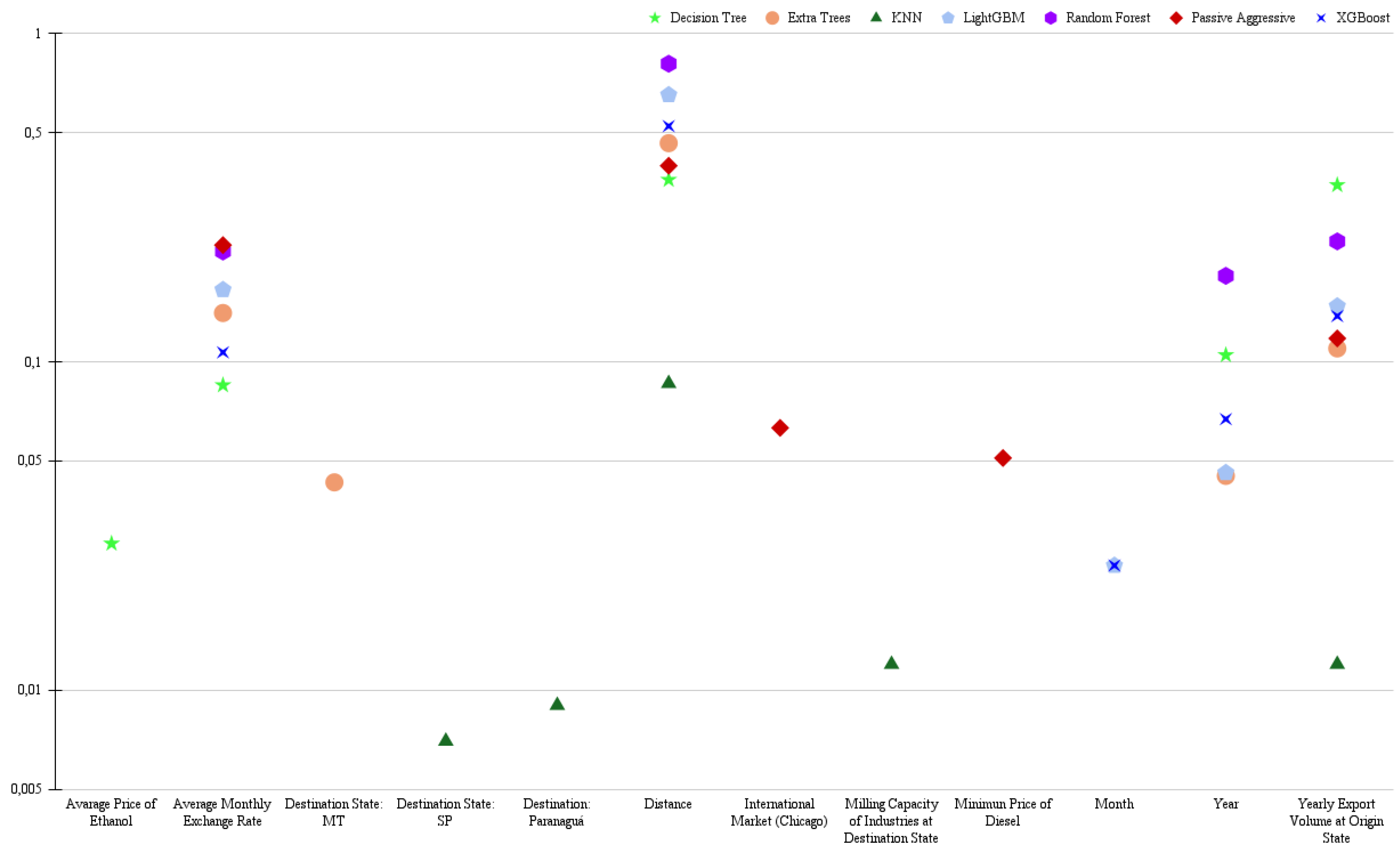
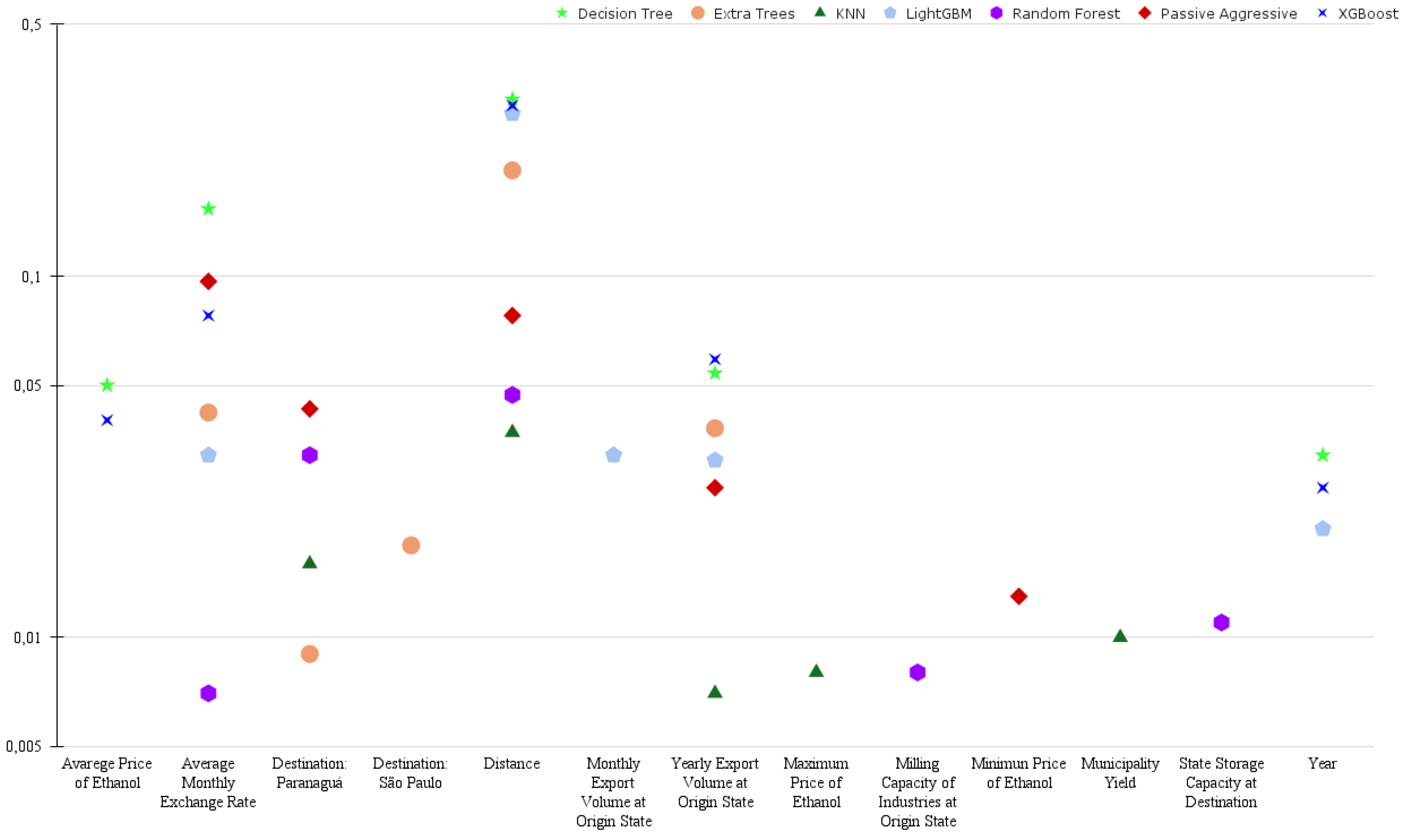
The analysis of predictive variables in regression and classification models, using the unstratified dataset (i.e., the complete dataset $\mathcal{D}$), revealed the predominance of the "Distance" variable as the most influential factor in determining the price of soybean road freight. This finding aligns with the expectation of direct influence in this process, as there is a clear relationship with operational costs such as fuel expenses, travel time, tire and parts wear, maintenance, and labor. The "Average Monthly Exchange Rate" and "Export Volume at Origin State" emerged as the second and third most relevant variables, respectively, highlighting the importance of the macroeconomic context of Brazilian soybean exports. The exchange rate directly influences the competitiveness of the product in the international market, affecting demand and, consequently, export volume. The export volume, in turn, impacts the demand for road freight to transport the production to export ports. Furthermore, in the evaluated models, we observed the presence of similar variables in both scenarios, namely: "Year", "Milling Capacity of Industries at Destination State", "Destination to Paranaguá", "Average Price of Ethanol", and the "Destination State: São Paulo" (Figure 1 and Figure 2).

The variable "Year" can capture macroeconomic trends, structural changes in the domestic market, and regulatory adjustments, such as the Truckers’ Law - Lei dos Caminhoneiros (Law No. 13,103/2015), which regulated aspects like working hours, rest periods, waiting times, and the establishment of a minimum floor for freight rates. Additionally, this variable may reflect specific events, such as the 2018 truckers’ strike, which halted cargo transportation nationwide, especially impacting the agricultural sector (Kreter et al., 2018).

Also pointed out as an influential variable, the "Milling Capacity of Industries" is a differentiating factor in soybean marketing, as the greater the milling capacity, the stronger the bargaining power (Martins et al., 2005). In contrast, soybeans that do not undergo industrial processing are largely destined for the external market. In this context, the Port of Paranaguá stands out as one of the main hubs for exporting Brazilian soybeans to the international market, especially to China. Its relevance on the national stage is comparable to that of other major export ports, such as the Port of Santos, located in São Paulo (USDA, 2024). The strategic location of the Port of Santosprovides insights into the importance of the "Destination State: São Paulo" variable in the analyzed models.

Figure 1. Five main variables resulting from the regression models.

Figure 1. Five main variables resulting from the regression models.

Figure 2. Five main variables resulting from the classification models.

Figure 2. Five main variables resulting from the classification models.

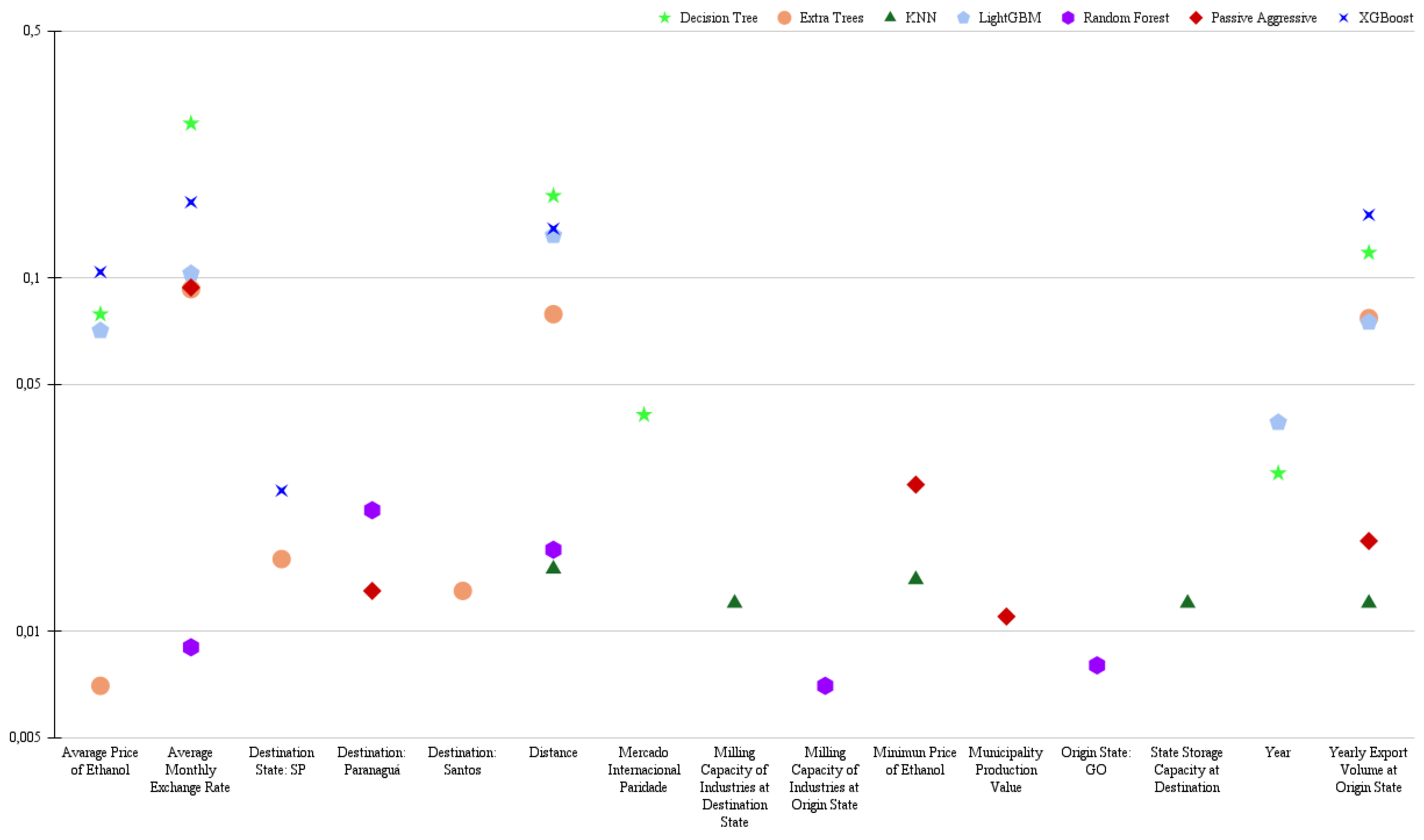
The data stratification revealed the influence of additional variables in determining the freight price for soybeans. The analysis of high freight rates (Figure 3) also highlights the influence of the "Yearly Export Volume at Origin State" variable, especially for the Decision Tree, ExtraTrees, and XGBoost models. Distance is particularly influential for the LightGBM and Random Forest models. The Volume of Exports by State of Origin per Year is especially relevant in the XGBoost and Decision Tree models. Variables related to the final destination suggest a correlation with the location of the main producing states, since for most of the period under study, Mato Grosso and Goiás, large soybean producers, used the Port of Santos as the main export route. In contrast, Paranáand Mato Grosso do Sul, also significant producers, directed their output to the Port of Paranaguá (COMEXSTAT, 2024).

Another variable that appears in high-value freight is "State Storage Capacity at Destination". Storage has a significant impact on the prices of agricultural commodities, as it allows for better marketing strategies (Delai et al., 2015). Specifically in the Brazilian scenario, the storage network does not keep pace with the dynamism of the sector, and there is a storage deficit, which leads to the so-called sales rush—when there is a peak in the harvest with a large supply of the product. At this time, soybean prices are low due to the abundant supply, while freight prices are high. Storage is essential for the transfer of production to processing and export centers since Brazil’s main soybean-producing areas are located far from export ports (de Lima et al., 2017). Innovative strategies, such as rural storage cooperatives, are being adopted by producers to reduce costs and improve logistical efficiency (Filippi and Figueiredo, 2019).

The variable "International Market (Parity)" which refers to the relationship between domestic soybean prices and international prices, is relevant in the KNN and LightGBM models. Price parity directly impacts producers’ marketing strategies, influencing their bargaining power with companies.

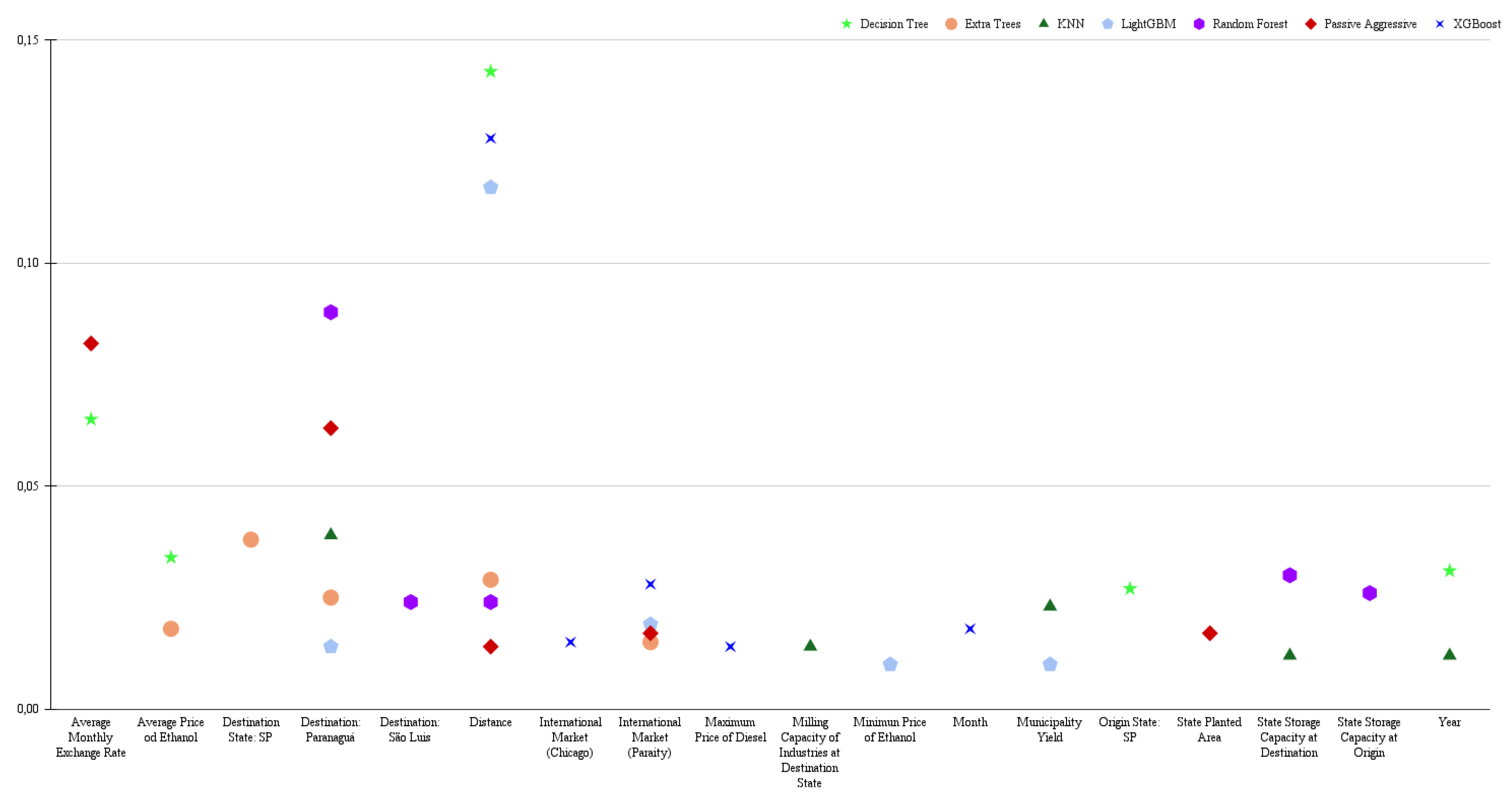
Similar to high freight rates, the average freight rate (Figure 4) also highlights the importance of the final destination, such as the Ports of ParanaguáandSão Luis, which are located closer to the main soybean-producing areas, unlike the Port of Santos. The Port of São Luis, in particular, has become increasingly relevant for soybean exports from Mato Grosso, with international destinations such as Hamburg, Germany, and Shanghai, China. The increased use of the Arco Norte routes, including São Luis, has been an efficient alternative to reduce logistical costs and ease the burden on southern ports, improving competitiveness in the global soybean market (USDA, 2024).

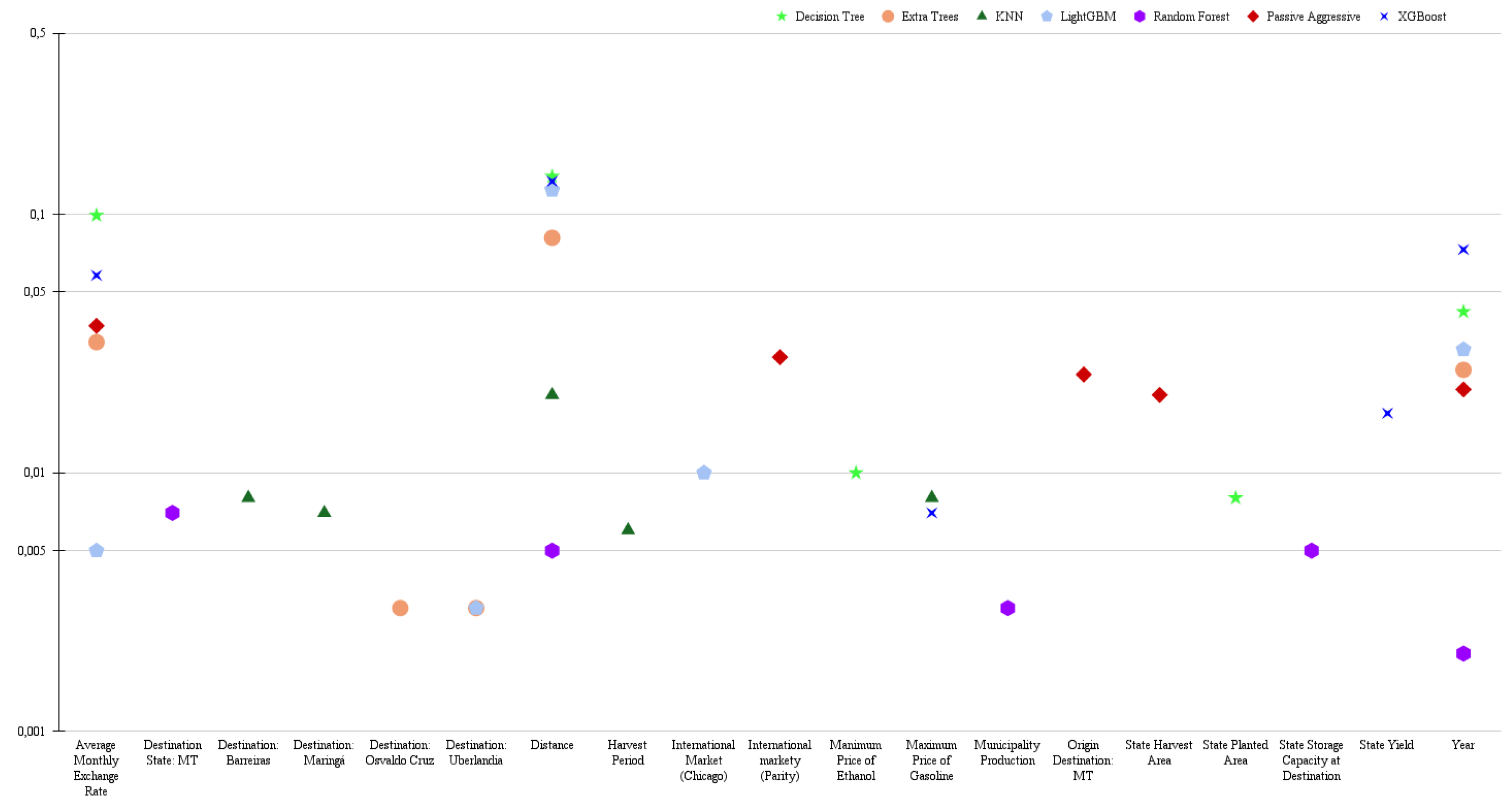
In short-distance freight (Figure 5), we observe a different scenario from that of medium and long-distance freight. While long-distance freight clearly indicates the transportation of soybeans destined for export, short-distance freight is more associated with domestic supply. The four cities that appear as short-distance destinations — Barreiras,Maringá, Osvaldo Cruz, and Uberlândia — have soybean crushing facilities (ABIOVE, 2024), dedicated to the production of oil and meal, products widely used in animal feed and biofuel production in the domestic market.

The stratification of the database, using the same models, highlighted the influence of freight rate division on the relevance of predictive variables. While the general scenario analysis identified 13 variables with significant influence, the segmentation by price ranges revealed a gradual increase in this number: 15 variables in the high freight scenario, 18 in the medium freight price scenario, and 19 in the low freight price scenario. The variables "Year," "Average Monthly Exchange Rate," "Distance," and "Minimum Price of Ethanol" consistently proved to be influential across all scenarios, suggesting their fundamental importance in determining freight costs, regardless of the price range. This variation in the number of relevant variables in each stratum demonstrates that stratification allowed for a more granular analysis, capturing the influence of different variables in each price range and reaffirming the dynamics of the freight market.

Lastly, grain transportation in Brazil, such as soybeans, generally begins with road transport, connecting farm production to final destinations, such as industries or export ports. In some cases, the cargo is initially sent to warehouses or transshipment terminals, from where it proceeds to the final destination via other transport modes, such as railways or waterways. This intermodal system aims to reduce costs and optimize the logistics of production flow. Although distance is a determining factor in the road freight price for agricultural products, the negotiation process between market agents has a fundamental impact. The grain transport market is highly competitive, marked by an imbalance of power between demand, represented by agricultural trading companies, and supply, composed of small transport companies and independent truck drivers. The trading companies, mostly transnational corporations, use their large cargo volumes to negotiate better freight conditions, taking advantage of the fragmentation among transport providers.

Additionally, the behavior of commodity markets, such as soybeans, is complex and can be influenced by various factors over time. During certain periods, different elements can determine the prices of these commodities, such as the availability of soybeans in the off-season (Ghalayini, 2017). Many forecasting models use only the historical prices of commodities (Drachal, 2018), but large price fluctuations can impact not only production and consumption costs but also government regulatory policies (Guo et al., 2022).

5. Conclusions

Transportation is a crucial component in the final cost of soybeans, with a complex and non-linear relationship. The different variables associated with each price range of soybean freight emphasize the non-linearity of this behavior across the spectrum. When evaluating variable classification, the LightGBM model proved to be the most accurate, while XGBoost, Passive Aggressive, and LightGBM stood out in regression analysis.

Distance is the most significant variable in determining freight costs, aligning with operational expenses such as fuel and labor. The study advances the theoretical understanding by demonstrating that distance remains the primary determinant of freight prices, yet macroeconomic factors like exchange rates and export volumes significantly impact price variations across different logistic scenarios.

The findings also contribute to the theory of supply chain management by identifying the stratified impact of different variables depending on the distance of transport (short, medium, and long). This adds a nuanced perspective to the transportation cost theories, suggesting that different models should be applied depending on the scope of the supply chain. Short-distance freights are more related to domestic supply, such as transportation to soybean crushing plants for the production of oil and meal. In contrast, medium and long-distance freights are predominantly tied to export logistics.The segmentation of the dataset also highlighted an increase in the number of relevant variables for each price range, underscoring the importance of a more granular analysis to capture freight dynamics.

From a managerial perspective, the results provide actionable insights for logistics managers and transportation planners. Understanding that distance, exchange rates, and export volumes are key determinants of freight costs allows managers to better anticipate price fluctuations and strategically plan logistics operations. For instance, managers can optimize routing and scheduling decisions by considering not only the operational expenses but also macroeconomic indicators. This predictive capability can support decision-making processes, such as choosing optimal transport routes and timing shipments to minimize costs.

Moreover, the variables can interact with each other, meaning that the impact of one variable partially depends on the values of others. For instance, the influence of distance on freight costs can be amplified or reduced by factors such as road infrastructure and weather conditions. The inclusion of additional variables like these, along with public policies, can further enhance the analysis, providing a more detailed and accurate view of freight price formation.