Evaluation of Diagnostic Usefulness of Multivariate Classification Models Used in Research of the Risk of Scoliosis

Purpose: Medical experiments frequently involve observations of many variables. For instance, the results of a blood chemistry test are a set of such multivariate data. The study attempts to diagnose the occurrence of scoliosis based on the results of biochemical analyses of blood serum samples. Methods: The following hormones were measured: FSH, LH, E2, PROG, HGH and PTH. Osteocalcin, calcium, phosphorus and vitamin D were also measured. Discriminant analysis and decision trees were applied to determine which of the measured parameters would allow the studied set to be divided naturally into four groups of patients. Result: After such a division, these techniques allowed for prognoses, and thus, for assigning new data to the four classes. The results of advanced statistical analyses are presented as classification functions and in a graphical form as a decision tree, as well as a set of decision rules. The study showed that diagnosing scoliosis is possible based on five (LH, E2, PROG, calcium and osteocalcin) out of ten available results of biochemical measurements. Conclusions: Statistical analysis allowed for classifying new medical cases with high probability, which may even increase after new data are introduced into the dataset and corrected classification systems are generated.

Keywords:

Subject:

Public Health and Healthcare - Primary Health Care

1. Introduction

Adolescent idiopathic scoliosis (AIS) is one of the most commonly observed spine deformities in children and youth in clinical practice. Scoliosis Research Society (SRS) defines AIS as a three-dimensional deformity with a curvature greater than 10°. In girls aged between 10 and 15 years, the incidence of the deformity is 2–4% [1]. There are many diagnostic methods used to determine the magnitude and type of curvature [1,2,3]. Despite numerous hypotheses, the aetiology of AIS remains unknown [4,5,6,7,8,9,10]. Therefore, it seems important to develop methods of evaluating the risk of scoliosis occurrence and the progression of scoliosis.

Making diagnostic and classification decisions in medicine usually involves combining experience in treating similar cases, results of recent studies and the physician’s personal judgement. As with other areas, decisions made by the physician play a key role in the diagnostic process. Decision support systems may, therefore, become an important tool in this process. Discriminant analysis and decision trees are used by researchers from different fields to make decisions because these methods allow for a high accuracy of classification [11,12,13,14,15]. Available results of diagnostic research may be used to design classification systems for assessing the risk of scoliosis [16,17,18].

2. Material and Methods

2.1. Results of the Conducted Research

The study was conducted with a group of girls who were patients of the University Hospital of Orthopaedics and Rehabilitation in Zakopane (Poland). In total, the study encompassed 200 girls aged between 11 and 19 years. The girls were divided into four groups of 50 each. The first group comprised non-menstruating girls with scoliosis (50 girls, 12.7 years) and the second group comprised menstruating girls with scoliosis (50 girls, 14.6 years). Two control groups were: non-menstruating girls (50 girls, 11.9 years) and menstruating girls (50 girls, 13.6 years). The selection criterion was scoliosis in the experimental groups and a correct body posture (after injuries only if not related to spine deformity) in the control groups.

In the girls with scoliosis, the spine curvature angle measured with the Cobb method was greater than 15°. Idiopathic scoliosis was diagnosed after a physical examination and evaluation of a radiograph in the AP plane conducted every six months. All biochemical analyses were conducted on blood serum samples left after routine tests. The samples were frozen and stored at a temperature of -80 °C until such time as they were measured. In the case of all menstruating girls, the study used blood samples collected between the second and third day after the end of menstruation. The following parameters were measured: follicle-stimulating hormone (FSH), luteinising hormone (LH), oestradiol (E2), progesterone (PROG), human growth hormone (HGH), parathyroid hormone (PTH), osteocalcin, calcium, phosphorus and vitamin D.

The diagnostic system will be created in two stages, the first stage will involve constructing a classifier and using cases comprising the learning (training) set, marked with the label Construction. The correctness of the functioning of the classifier will be checked with the cases marked with the label Evaluation. For each of the four groups of girls, five such cases were drawn, forming a testing set of 20 elements.

The permission to conduct the tests planned for the experiment was granted by the Bioethics Committee. The permission included a form for the informed consent of patients.

2.2. Statistical Methods Used to Analyse the Obtained Results

The results of the conducted research were analysed with the following statistical methods: descriptive statistics, discriminant analysis and classification trees.

2.2.1. Descriptive Statistics

Data analysis began with the graphical representation of data, which provided a goodly amount of interesting information about the structure of the studied sets. The first stage of the analysis involved analysing the variables with respect to the occurrence of outliers and substituting distant values with mean values. This operation was essential because the classification methods used in this study are very sensitive to outliers. To evaluate the sets of laboratory data graphically, scatterplots, probability plots, and categorised graphs were used. Scatterplots were used to visualise the relationships between the studied variables. Probability plots were used to estimate the normality of distribution of the variables. The overview of the selected variables, determined by two (girls with and without deformities) or four categorising variables (four groups of studied children), was visualised using categorised graphs.

For the purpose of synthetic description of the datasets, two scatterplots were used: box-and-whisker plots, constructed to depict the measures of location, dispersion and asymmetry in the analysed dataset, and histograms, which present the frequency distribution of the studied variable. Furthermore, the values of these measures were determined.

2.2.2. Discriminant Analysis

Discriminant analysis is applied to decide which variables describing objects discriminate two or more naturally distinguishing groups. In medical research, different biochemical parameters of patients may be registered in patients to test which of the parameters is optimal for classifying the patients into groups. The main idea underlying discriminant analysis is the possibility of analysing several variables simultaneously, in order to indicate optimal variables for determining membership in one of a few possible groups. Discriminant analysis begins with procedures describing and interpreting differences between groups, followed by procedures for classifying cases, that is, determining which group the case belongs to, based on the values of characteristics obtained though observation and experience. The task simply involves determining canonical discriminant functions separating the studied groups. If the groups vary, then each of the groups may be treated as a cloud of points in a space with axes that are discriminant variables. These clouds of points may slightly overlap each other, but the majority of points are located in centroids distant from each other. A centroid denotes a fictional point, the coordinates of which equal the mean group values of each discriminant variable. It is assumed that centroids are typical representatives of each group.

The main aim of discriminant analysis is to predict which group a classified case belongs to. All classification procedures involve a comparison of the location of the case in relation to each calculated centroid, performed in order to find the closest centroid. The classification process is connected with constructing one or several functions, which classify the analysed cases into appropriate groups, based on a linear combination of discriminant variables (R. Fisher). For each i-th group, Fisher introduced a separate linear combination in the following form:

K_i = c _io ₊ c _i1*x₁ + … + c _i_j*x_j ,

where: cij, j = 0,1, …, n are coefficients calculated from discriminant variables for each classification function. There are as many functions as there are groups (i = 1, 2, …, g).

These classification functions are used to decide which group a given case most likely belongs to. Under such definitions of functions, a given case is classified to the group for which K_i assumes the highest value.

Discriminant analysis can be divided into two stages:

learning stage, during which classification rules are created based on the training set (research results);
classification stage, during which the established characteristics of classes determine which class the objects belong to.

Usually, the classification of the set of cases that served as the basis for developing discriminant functions is more accurate than the classification of the cases that were not used in estimating discriminant functions. To evaluate the usefulness of classification equations, a dataset is divided into two subsets: learning and testing (if the sample is large), or new data should be gathered, to test the accuracy of classification.

In the case of this study, discriminant analysis was used to investigate the membership of the studied girls in one of the four classification groups.

2.2.3. Classification Trees

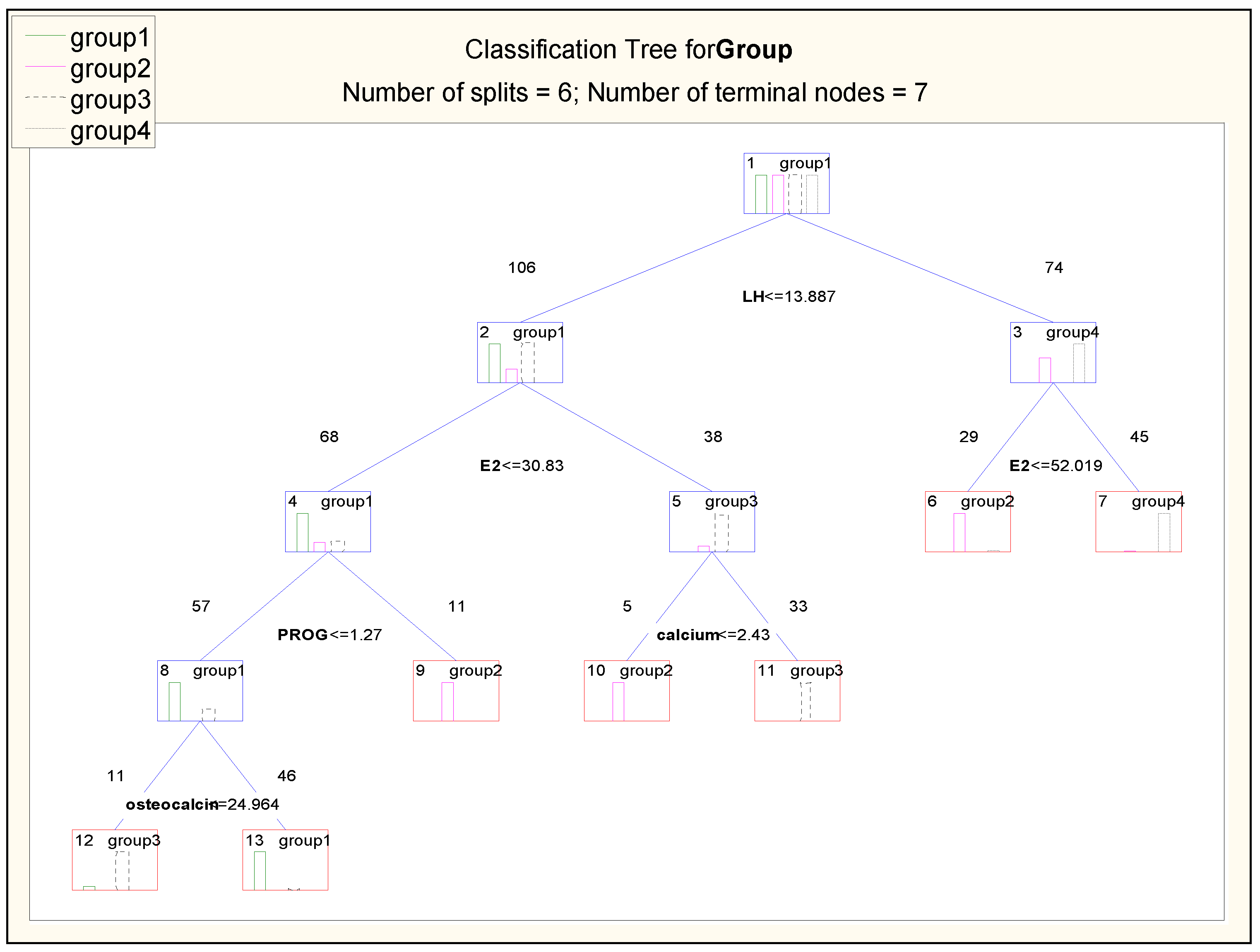
Today, traditional methods of data analysis are more and more often replaced by special methods of modelling, and data mining continues to gain popularity. This is because these methods can recreate almost any relationship occurring between variables, as long as a good amount of high-quality data is available. One of the most typical methods of data mining are classification trees, which are commonly used in fields such as botany (classification) and medicine (diagnosis). Graphical presentation of knowledge about a research process in the form of a tree makes interpreting results easier that is the case with purely numerical results. Trees are used to assign cases and objects to classes of a qualitative dependent variable based on measurements of one or more explanatory variables (predictors, attributes). The STATISTICA software [19,20] allows for constructing a tree through an exhaustive search for the division of cases into classes. The algorithm is a complete interpretation of techniques of calculating binary classification trees based on univariate divisions. A classification system is presented in the form of a decision tree, which comprises nodes and branches (Figure 6). The root node of a decision tree is the first node in a classification diagram, located the lowest. Logical conditions, denoting the criterion of division, are located between the branches of a tree, and numbers located above the nodes provide information about the number of observations in a child node, the number of the node and the predicted class to which the majority of the cases, represented by a histogram, belong. In each node, the majority class (the label of the predicted class) is provided; this is the class to which the majority of the elements of the learning subgroup that are located in the node belong. The number of elements in classes is represented by the height of the bars in the histogram.

As with Discriminant analysis, the base of medical cases is divided into the training set and the testing set, which is used to check the correctness of the created classification tree. Prediction accuracy is analysed by using the constructed decision tree to determine the class membership in a validation sample, which comprises the results of the research not taken into account during the learning stage. When constructing a tree, V-fold cross-validation may additionally be used. The aim of this method is to obtain a tree of appropriate size. This test involves a random division of learning data into several parts and investigating predictive accuracy for the trees trained on random data subsets. Decision trees may be converted into a base of decision rules.

The aim of the analysis based on classification trees is to correctly predict and explain the responses (reactions) codified in a qualitative dependent variable, and for this reason, the techniques used in this module have much in common with the techniques used in more traditional statistical methods, such as discriminant analysis. This study uses both methods and compares the obtained results.

3. Results

3.1. Graphical Presentation of Results. Statistical Measures

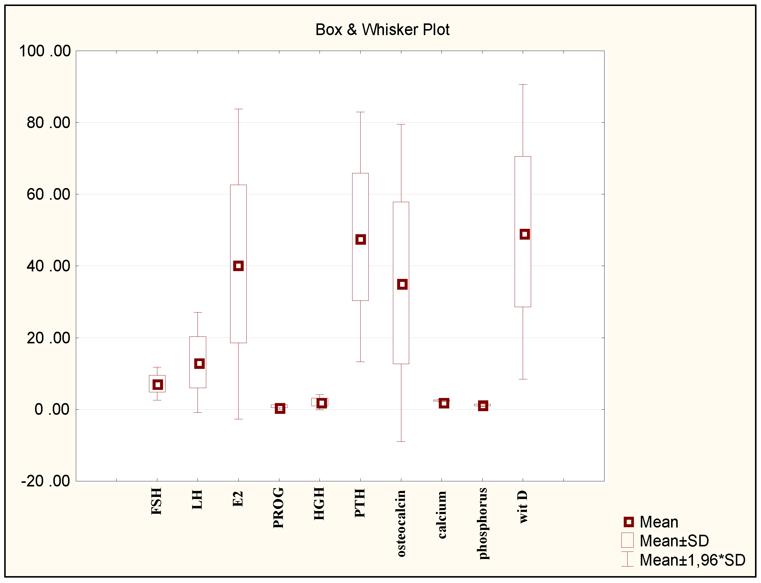
Graphics plays a very important role in statistics. Any result of calculations becomes clearer and more understandable when represented in a graphical form, especially for persons using statistics as a supporting tool in their work. The plot illustrating the ranges of the studied variables is presented in Figure 1.

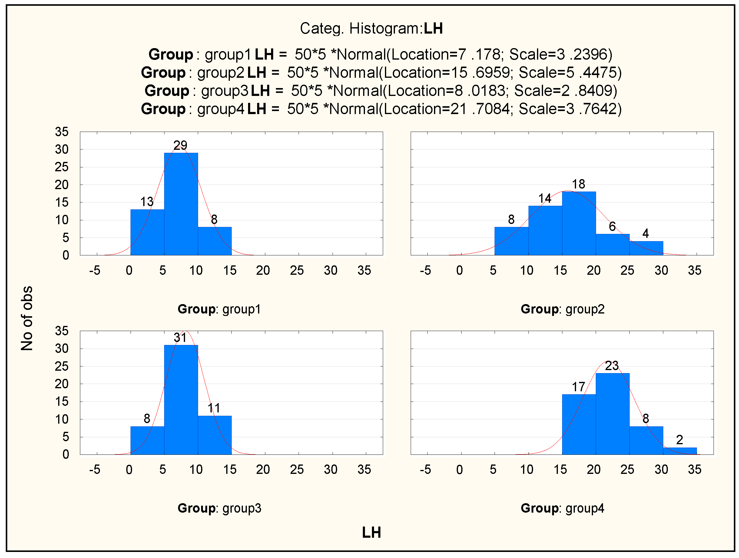
For all analysed variables, box-and-whisker plots were constructed, as well as histograms for variables and, additionally, histograms for categorised variables (Figure 2). Sample results are presented in Figure 2 and Figure 3.

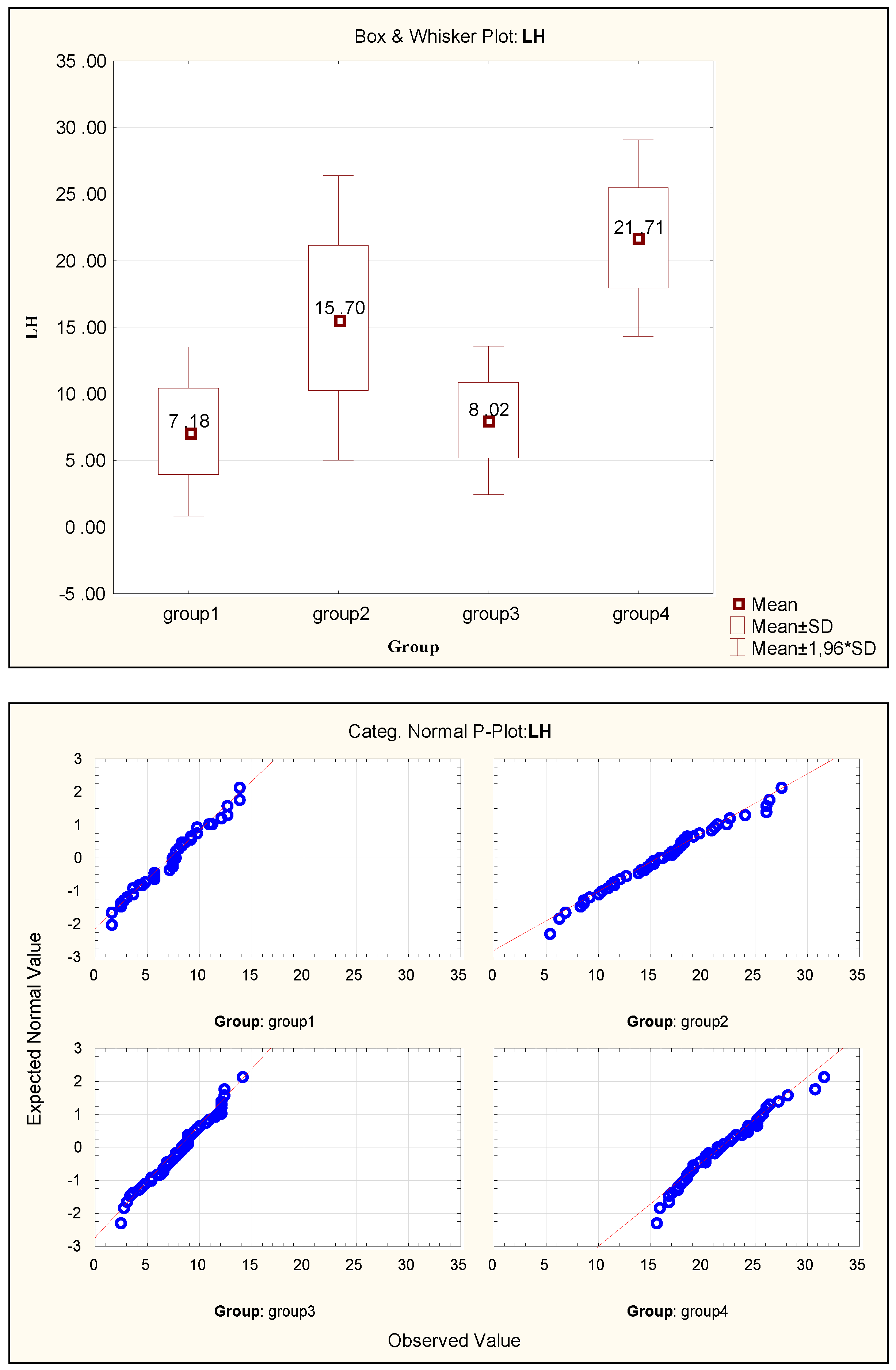
Figure 3 present scatterplots of the mean value with marked standard deviation and normality plots for the same variable, constructed separately for all studied groups.

In order to investigate the normality of the obtained histograms, the Shapiro-Wilk W-test was conducted. The results of the assessment of the normality of the categorised distributions of the variables were used for the conducted discriminant analysis.

3.2. Discriminant Analysis

Discriminant analysis was conducted using the STATISTICA package. The modules for discriminant analysis make this software an extremely effective tool for classification and data mining techniques. These analyses are part of the module Multivariate exploratory techniques. The Group variable, which unambiguously assigned the cases (the studied patients) to four groups (group 1, group 2, group 3, group 4), was selected as the grouping variable. The provided list of 10 independent variables (the list of measured hormones) includes the results of the conducted research.

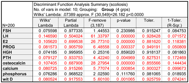
In the next step, the variables that are the most useful for discriminant analysis were indicated (Table 1).

It can be concluded that seven variables, the significance of which was confirmed by the calculated values of p (p << 0.05), should be selected for further analysis. The variables FSH, HGH, and phosphorus, for which p > 0.1, will be excluded.

To enable both stages of discriminant analysis, the dataset was divided randomly. From each groups of girls, five cases were drawn, which formed the testing group. The remaining 180 cases were taken into account as the learning set that was used to construct classification functions. For this purpose, the module Traditional discriminant analysis was selected in the STATISTICA software. The purpose of discriminant analysis was to check whether it was possible to assign a given child to one of the four defined groups based on the values of the seven biochemical parameters measured for each group.

Table 2 shows the results of the calculations, the analysis of which allows for determining which discriminant functions are statistically significant.

Canonical discriminant functions were developed by calculating their coefficients. In order to indicate which groups are best discriminated by each function, mean values for discriminant functions were calculated.

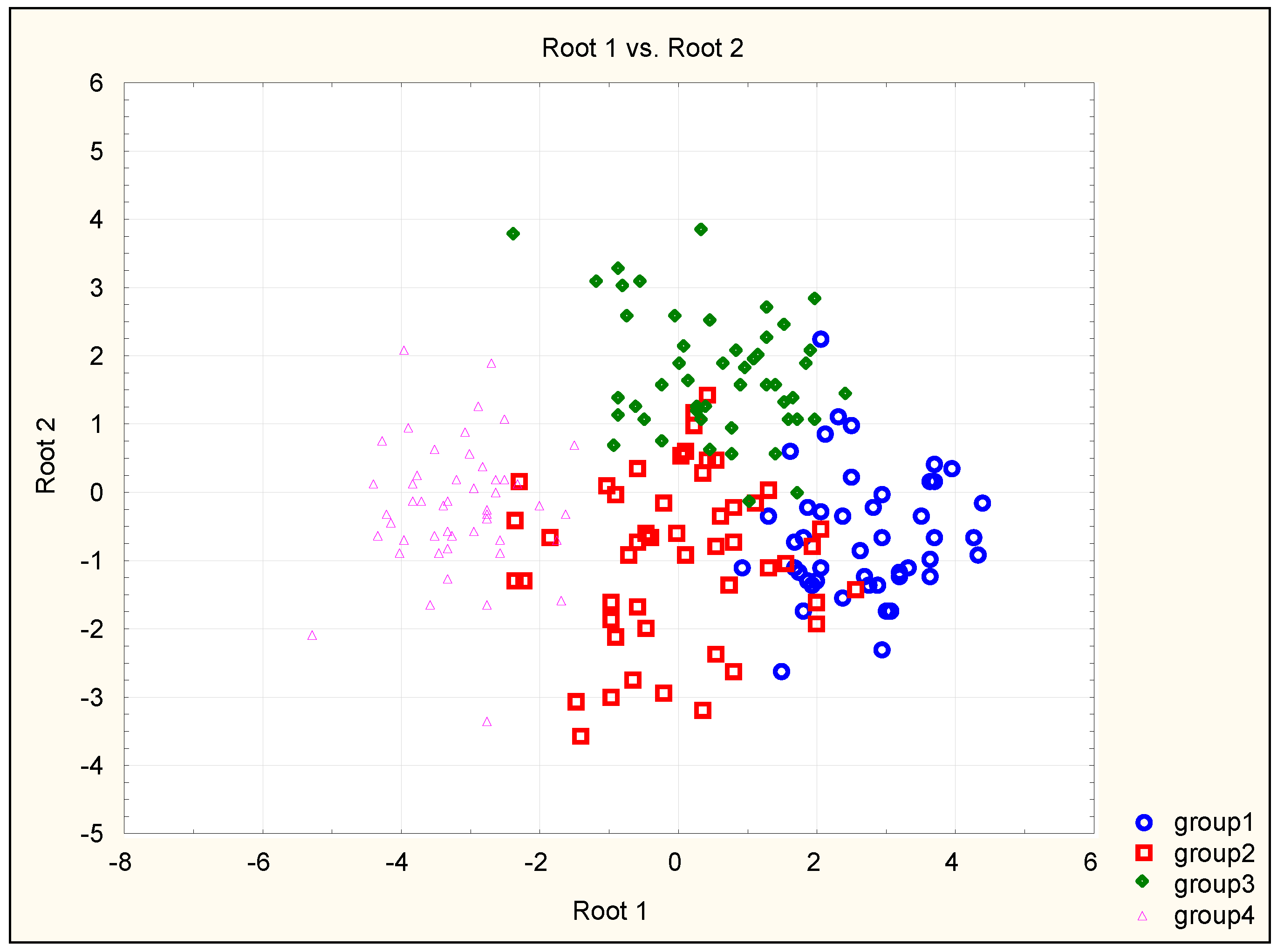
For the first two developed discriminant functions, the scatterplot of canonical values (Figure 4) was constructed, which shows the overlapping of the four studied groups of patients. It can be observed that group 4 is the most isolated one, and group 2 is the least isolated one.

Classification procedures can be initiated after determining and testing the significance of discriminant functions. The algorithm of classification of objects is initiated by selecting the Classification.

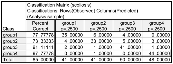
The results of the correctness of classification for the learning set (180 cases) are shown in Table 3. The classification matrix presented in the table contains information about the number and percentage of objects (cases) correctly classified in each group.

The developed functions K₁, K₂, K₃, K₄ allow for classifying new cases. For each case, values of all classification functions are calculated. A patient (case) is assigned to the group with the highest value of the classification function. In order to test the effectiveness of the established classification functions, the cases from the testing set were classified, that is, the cases which were not used to calculate the coefficients of the functions K₁, K₂, K₃, K₄.

The mean percentage of correctly classified patients is slightly lower than the result obtained for the learning set and equals 80% of the overall number of the studied girls.

Further research assumed that an additional classification method will be used to build a diagnostic system, that is, decision trees.

3.3. Classification Trees

The STATISTICA software was used to build a decision tree allowing for the classification of the groups of the studied girls. The classification used the medians of the range of variability of the measured levels of hormones.

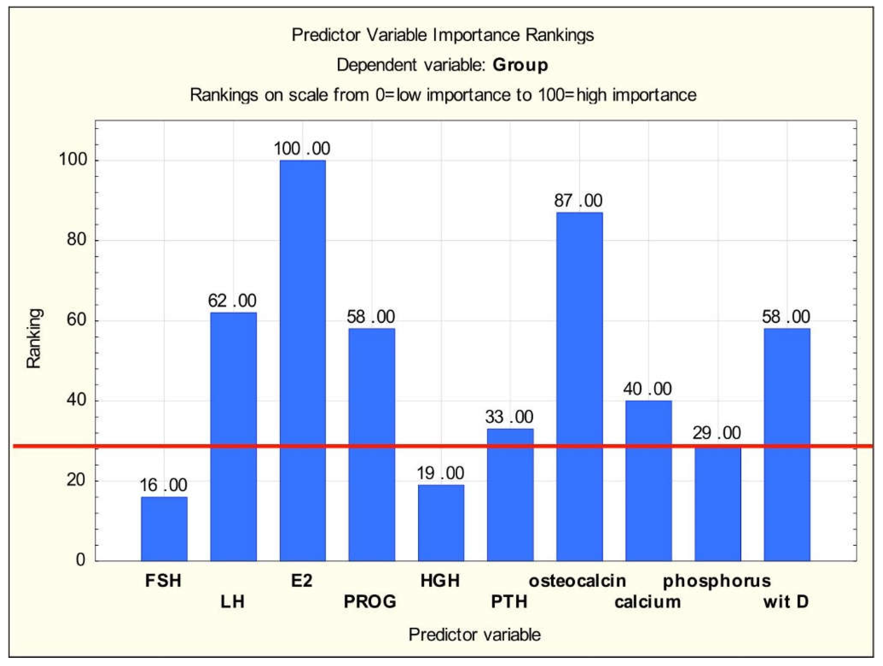
The decision tree was constructed for the variables describing 180 cases of randomly selected girls (the learning sample – used at the stage of building the decision tree), and 20 cases formed the testing group, which was used to evaluate the built tree. First, the significance of all 10 variables, which were the results of laboratory research, was evaluated. The results of the ranking are shown in Figure 5.

Only the top five variables from the ranking were selected for constructing the decision tree (as with the Discriminant analysis). The structure of the generated classification tree is shown in Figure 6.

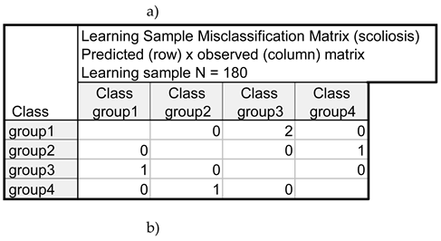
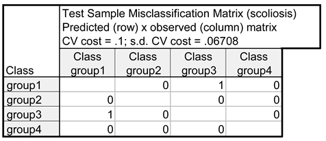
The headline of the figure (Figure 6) includes the number of divisions (6), which denotes the number of decision nodes (the number of questions in the system), and the number of terminal nodes (7), presented as the leaves on the tree and denoting the identified groups. In the subsequent nodes of the tree (the nodes were marked in blue), the set of cases is divided into subsets based on the conditions testing the values of the attributes. The terminal nodes (the leaves of the tree), which contain the decisions, that is, the type of the identified group, are marked in red. The classification effectiveness of the generated decision tree was tested for both the learning dataset and the testing dataset (Table 4).

4. Discussion

Graphical presentation of the obtained results is a very important stage of working with data acquired through research. Presenting the obtained results in a clear manner and in accordance with the commonly accepted rules makes it easier to choose the method of further processing the data and interpreting the results of experimental research correctly.

Also in the case of the present study, the analysis of source data began with the analysis of their graphical presentation. The study investigated two groups of patients: girls with scoliosis (group 1 and group 2) and girls without scoliosis (group 3 and group 4). Each of the groups is divided into two subgroups: girls who had not started menstruating yet (group 1 and group 3) and menstruating girls (group 2 and group 4).

The analysis of data began with the preparation of descriptive statistics characterising the studied groups. The plot presented in Figure 1 shows an overview of the values of the hormones measured for the studied groups of girls; it does not show the values of the measured parameters. The presented relationships (Figure 1) indicate a high diversification of the ranges of the measured hormones, which usually results in the necessity of using the procedures of data normalisation when conducting, for instance, discriminant analysis. Basic statistical parameters were calculated for each variable characterising the studied groups of patients. The results are described in more detail in the authors’ previous articles [8,9]. In this study, Figure 2 and Figure 3 present only some of the obtained results, focusing on the LH variable, which was found to be the parameter considered the most diagnostic one in the further statistical analyses conducted. Such histograms may be a combination of several separately calibrated distributions. For each value of categorised variable (experimental group), a separate frequency distribution can be drawn. The categorised histogram for the results of the measurement of the luteinising hormone is presented in Figure 2. Figure 3 show scatterplots of the mean with marked standard deviations determined for all four studied groups of patients and the plot of probability distribution for the same variable. The results presented in Figure 3 show that the variation values of the analysed trait differ considerably from each other in each of the studied groups, which suggest that there are significant differences between the mean values in the analysed groups. The Shapiro-Wilk W-test conducted for the LH variable confirms that the distribution of this categorised variable is normal because in all studied groups p > 0.05. For the measurements of other biochemical data, confirming the normality of the categorised distributions of the variables was possible in the majority of cases. For several variables, the study observed slight departures from normal distribution (at the ends of the range of variability). The obtained tests of significance, however, remain reliable, because the samples are numerous, and the lack of normality results only from the skewness of the histogram showing the data distribution.

Normality of the distributions of variables is usually tested prior to more advanced statistical analyses. The present study used two methods implemented into the STATISTICA package: discriminant analysis and decision trees. The methods are qualified by the software as Multivariate exploratory techniques.

The preliminary results of the conducted discriminant analysis confirmed that discrimination of the membership in a group is highly significant. This is indicated by the value of Wilks' lambda, which equals 0.0738851, and the approximate value of F, which equals 26.18207, and the corresponding value of p < 0.05. Also indicated were the variables, which are the most useful in discriminant analysis. The analysis of the results presented in Table 4 allows for forming a conclusion that seven variables, the significance of which was confirmed by the calculated values of the p parameter (p << 0.05), should be selected for further analysis: LH, E2, PROG, PTH, osteocalcin, calcium and vitamin D. The following variables, for which p > 0.1, will be excluded are FSH, HGH, and phosphorus. The significance of discriminant functions was also confirmed. As can be seen (Table 2), the first two functions are characterised by a high value of canonical correlation R. This indicates a strong relationship between the groups of patients and discriminant functions. The first row in the table contains the significance test for all roots. The second row contains the results of the evaluation of the significance of roots that remained after removing the first root (etc.). Because the p values for all three discriminant functions are very close to 0, all functions were found to be significant. Therefore, it can be said that the results of the conducted research come from the population, where four groups of the studied patients (the number of significant discriminant functions is equal to the number of groups) emerge naturally. The obtained results were compared with each other in order to determine the size and direction of the shares of the variables in each canonical discriminant function. For example, the variables LH and E2 have the strongest impact on the first function, and this impact is very similar (both coefficients are negative and equal -0.567 and -0.508, respectively). The first function is responsible for 75.4% of the explained variance. This means that 75.4% of the entire discriminatory power is explained by this function, and this is why the first function is the most important one. The second function explains 21.2% and the third function explains only 3.4% of discriminatory power. This is confirmed by the earlier results, namely, the value of the canonical correlation coefficient R for the third function equals only 0.397 (Table 2).

The presented results of the calculations of the mean values of discriminant functions indicate that the first discriminant function differentiates primarily the objects from group 4 and, to a smaller degree, the objects from group 1. The second discriminant function seems to distinguish the third group, but, as can be seen, the value of this discrimination is considerably lower. The situation is confirmed by the scatterplot of canonical values shown in Figure 4. It can be observed in the figure that the girls from group 4 (without scoliosis, menstruating) are located significantly more to the left than the other groups and create a distinctive cluster. This discriminant function is affected the most by the LH and E2 variables. The higher the values of these variables are, the more to the left the object is located (unambiguously belonging to group 4). Similar interpretation may be applied to the second discriminant function, on which the LH and osteocalcin have a strong positive effect, and which can be used to test the membership of objects in group 3. The cases belonging to group 2 are located within all the remaining groups.

The classification of cases is possible after developing classification functions. The equations presenting the classification functions have the following form:

K₁ = -121.671 + 0.497*LH + 0.300*E2 + 4.893*PROG + 0.043*PTH +
+ 0.204*osteocalcin + 81.762*calcium + 0.200*Vit D

K₂ = -122.862 + 0.986*LH + 0.369*E2 + 6.727*PROG + 0.043*PTH +
+ 0.119*osteocalcin + 80.102*calcium + 0.208*Vit D

K₃ = -133.221+ 0.371*LH + 0.452*E2 + 5.143*PROG + 0.100*PTH +
+ 0.048*osteocalcin + 85.804*calcium + 0.226*Vit D

K₄ = -158.706 + 1.242*LH + 0.530*E2 + 9.631*PROG + 0.071*PTH +
+ 0.065*osteocalcin + 86.339*calcium + 0.291*Vit D

The assessment of the usefulness of the established classifiers was verified for the training set and the testing set. The results of the correctness of classification for the learning set (180 cases) are presented in Table 3. The classification matrix presented in the table contains information about the number and percentage of objects (patients) classified correctly in each group. The highest percentage of correctly classified cases is observed in the group of healthy girls, that is, in group 4 (97.8%) and group 3 (91.1%). The percentage of correctly classified girls with scoliosis equals 77.8%, for group 1 (non-menstruating girls) and 73.3%, for group 2 (menstruating girls). The obtained results match the areas of the overlapping of the objects belonging to the different classes observed in Figure 4. It can be observed that group 4 is the most isolated one and group 2 is the least isolated one. In the case of group 2, the calculated percentage of incorrectly classified patients is the highest and equals 26.7%. The established functions K₁, K₂, K₃, K₄ allow for classifying new cases from the testing set, which were not used for calculating the coefficients of the functions. The mean percentage of correctly classified patients is slightly lower than the result obtained for the learning set and equals 80% of the overall number of the studied girls. The worst result of the correctness of classification (both for the learning group and the testing group) was obtained for the patients belonging to group 2. Such a result can be explained by the fact that this group is characterised by the highest dispersion of the values of the measured biochemical parameters (Figure 3). Furthermore, assigned to group 2 were girls aged between 11 and 19 years, and the age difference between the children from the other groups is only 5 or 3 years. Such high differences in the age of the children in group 2 probably had an effect on the correctness of classification.

In order to compare the classification capabilities of various calculation methods, a diagnostic system was constructed, which was represented by a decision tree. The tree was also built using the STATISTICA software. First, analogously as in the case of Discriminant analysis, the significance of all 10 variables, which were the results of the laboratory research, was evaluated. The results of the ranking (Figure 5) confirmed that FSH, HGH and phosphorus (in the figure, they are separated off by the red line) should be considered less significant if a construction algorithm for decision trees is used to create a classifier. The same conclusion was formulated in the case of discriminant analysis, which was discussed earlier (Table 1). For this reason, only the top seven variables from the ranking were selected for constructing the decision tree.

The structure of the generated tree is presented in Figure 6. The root of the tree contains the LH attribute, which possessed the ‘largest amount of diagnostic information’, that is, the values of the attribute allowed for distinguishing from the studied set the majority (74) of menstruating girls (29 girls from group 2 and the entire group 4), which finds confirmation in the physiological levels of this hormone in women on their period. Then, the tree was constructed recursively, in accordance with the principle of locating the attributes bringing the highest information gain in the root, guaranteeing the most optimal division of the studied sample. In the obtained classification system, the LH variable was found to be the most important decision attribute, followed by E2, PROG, calcium, and finally, osteocalcin. Node no. 5 contains a question about the level of calcium, the value of which allows for distinguishing the group of menstruating girls with scoliosis (5 persons from group 2) from those without scoliosis (33 persons from group 3). In node no. 8, the calculated value of the osteocalcin parameter allows for indicating which of the non-menstruating girls form group 1 and which belong to group 3. The analysis of the content of the nodes that are the leaves of the tree allows us to conclude that groups 4 and 1 are sets better isolated than the other ones because there is only one decision pathway leading to them. To classify a case belonging to group 3 two pathways have to be analysed and classifying a case belonging to group 2 requires analysing three decision pathways.

The results presented in the form of a classification tree may be converted into a set of rules and used in this form in the process for prognosing the classes for new medical cases. The rules allowing for classifying the studied girls into appropriate groups may be formulated as conditional sentences:

Rule 1: IF ((LH ≤ 13.887) AND (E2 ≤ 30.83) AND (PROG ≤ 1.27) AND (osteocalcin > 24.964)) THEN group 1

Rule 2: IF (((LH > 13.887) AND (E2 ≤ 52.019)) OR ((LH ≤ 13.887) AND (E2 ≤ 30.83) AND (PROG > 1.27)) OR ((LH ≤ 13.889) AND (E2 > 30.83) AND (calcium ≤ 2.43))) THEN group 2

Rule 3: IF (((LH ≤ 13.887) AND (E2 ≤ 30.83) AND (PROG ≤ 1.27) AND (osteocalcin ≤ 24.964)) OR ((LH ≤ 13.889) AND (E2 > 30.83) AND (calcium > 2.43))) THEN group 3

Rule 4:IF (LH > 13.887) AND (E2 > 52.019) THEN group 4

Using the rule knowledge base and software operating as an inference engine (e.g. SCANKEE [21,22]) allows for a full automation of the process of diagnosing scoliosis cases and makes it easier for a physician managing a patient to make a decision about treatment and rehabilitation.

The results of the assessment of the correctness of classification by the constructed decision tree (Table 4) and the base of rules developed based on the tree lead to the conclusion that out of 180 cases forming the learning set, five girls were classified in the incorrect group. As far as the set of 20 girls forming the testing set, two persons were classified incorrectly. Thus, the effectiveness of classification of the generated decision tree equals 97.2% for the learning set and 90%, for the testing set. Both results are better than the results obtained as the outcome of discriminant analysis.

5. Conclusions

The conducted research confirmed that the level of the selected hormones has a significant effect on the occurrence of scoliosis. Diagnosing scoliosis is possible based on five results of biochemical measurements (LH, E2, PROG, calcium, osteocalcin). Statistical analysis allowed for classifying new medical cases with high probability, which may even increase after new data are introduced into the dataset and corrected classification systems are generated. Drawing from published research results,[23] it is possible to select a testing procedure useful for choosing appropriate methods of actualisation for the previously developed predictive models and add new cases of diagnosed scoliosis to the learning set and the testing set.

Conflicts of Interest

The authors have no conflicts of interest to declare.

References

Horne, J.P.; Flannery, R.; Usman, S. Adolescent idiopathic scoliosis: diagnosis and management. Am Fam Physician 2014, 89, 193–198. [Google Scholar] [PubMed]
Qiu, Y.; Zhu, F.; Wang, B.; Yu, Y.; Zhu, Z.; Qian, B.; Zhu, L. Clinical etiological classification of scoliosis: report of 1289 cases. Orthop Surg 2009, 1, 12–16. [Google Scholar] [CrossRef] [PubMed]
Ng, S.Y.; Bettany-Saltikov, J. Imaging in the diagnosis and monitoring of children with idiopathic scoliosis. Open Orthop J 2017, 11, 1500–1520. [Google Scholar] [CrossRef] [PubMed]
Tang, S.P.; Cheng, J.C.Y.; Ng, B.K.W.; Lam, T.P. Adolescent idiopathic scoliosis (AIS): an overview of the etiology and basic management principles. Hong Kong J Paediatr 2003, 8, 299–306. [Google Scholar]
Schiller, J.R.; Thakur, N.A.; Eberson, C.P. Brace management in adolescent idiopathic scoliosis. Clin Orthop Relat Res 2010, 468, 670–678. [Google Scholar] [CrossRef] [PubMed]
Adobor, R.D.; Riise, R.B.; Sřrensen, R.; Kibsgĺrd, T.J.; Steen, H.; Brox, J.I. Scoliosis detection, patient characteristics, referral patterns and treatment in the absence of a screening program in Norway. Scoliosis 2012, 7, 18. [Google Scholar] [CrossRef] [PubMed]
Zheng, Y.; Dang, Y.; Wu, X.; et al. Epidemiological study of adolescent idiopathic scoliosis in eastern China. J Rehabil Med 2017, 49, 512–519. [Google Scholar] [CrossRef] [PubMed]
Kulis, A.; Goździalska, A.; Drąg, J.; Jaśkiewicz, J.; Knapik-Czajka, M.; Zarzycki, D. Participation of sex hormones in multifactorial pathogenesis of adolescent idiopathic scoliosis. Int Orthop 2015, 39, 1227–1236. [Google Scholar] [CrossRef] [PubMed]
Goździalska, A.; Jaśkiewicz, J.; Knapik-Czajka, M.; et al. Association of calcium and phosphate balance, vitamin D, PTH, and calcitonin in patients with adolescent idiopathic scoliosis. Spine (Phila Pa 1976) 2016, 41, 693–697. [Google Scholar] [CrossRef]
Dastych, M.; Cienciala, J.; Krbec, M. Changes of selenium, copper, and zinc content in hair and serum of patients with idiopathic scoliosis. J Orthop Res 2008, 26, 1279–1282. [Google Scholar] [CrossRef] [PubMed]
Matusik, S.; Woźniacka, R. Model of long bones growth increase rate among children with different physical activity based on the decision trees method. Polish J Environ Stud 2007, 16, 371–374. [Google Scholar]
Dębska, B.; Dłuski, M. Attempt of assessment of relation between asymmetry of pelvis and shape of scoliosis. J Orthop Trauma Surg Rel Res 2013, 32, 25–35. [Google Scholar]
Shouman, M.; Turner, T.; Stocker, R. Using decision tree for diagnosing heart disease patients. In CRPIT Volume 121—Data Mining and Analytics; ACS: Ballarat, Australia, 2011; pp. 23–29. [Google Scholar]
Marshal, R.J. The use of classification and regression trees in clinical epidemiology. J Clin Epidemiol 2001, 54, 603–609. [Google Scholar] [CrossRef] [PubMed]
Dębska, B.; Guzowska-Świder, B. Decision trees in selection of featured determined food quality. Anal Chim Acta 2011, 31, 261–271. [Google Scholar] [CrossRef] [PubMed]
Kloss, S.S.; Liu, X.C.; Lyon, R.M.; Tassone, J.C.; Thometz, J.G. Reliability of a functional classification system in the monitoring of patients with idiopathic scoliosis. Spine (Phila Pa 1976) 2007, 32, 1662–1666. [Google Scholar] [CrossRef] [PubMed]
Liu, X.C.; Thometz, J.G.; Lyon, R.M.; Klein, J. Functional classification of patients with idiopathic scoliosis assessed by the Quantec system: a discriminant functional analysis to determine patient curve magnitude. Spine (Phila Pa 1976) 2001, 26, 1274–1278. [Google Scholar] [CrossRef] [PubMed]
Ramirez, L.; Durdle, N.G.; Raso, V.J.; Hill, D.L. A support vector machines classifier to assess the severity of idiopathic scoliosis from surface topography. IEEE Trans Inf Technol Biomed 2006, 10, 84–91. [Google Scholar] [CrossRef] [PubMed]
Stanisz, A. Intelligible Statistics Course Using STATISTICA PL, on Examples of Medicine. Part 3. Multivariate Analyses; StatSoft Poland: Krakow, Poland, 2009. [Google Scholar]
STATISTICA (Data Analysis Software System), Version 12. StatSoft, Inc. 2014. Available online: www.statsoft.com (accessed on 20 June 2018).
Dębska, B. Graphic-rules knowledge base in the SCANKEE expert system supporting medical diagnostics. In Computers in Medicine; Kącki, E., Ed.; Lodz University of Technology: Lodz, Poland, 1994; pp. 19–23. [Google Scholar]
Dębska, B.; Guzowska-Świder, B. Application of knowledge engineering program environment system "SCANKEE" for recognition of structural units in the molecule of an organic compound. J Mol Struct 1995, 348, 473–476. [Google Scholar] [CrossRef]
Vergouwe, Y.; Nieboer, D.; Oostenbrink, R.; et al. A closed testing procedure to select an appropriate method for updating prediction models. Stat Med. 2016, 36, 4529–4539. [Google Scholar] [CrossRef]

Figure 1. Ranges of the studied variables.

Figure 2. Histograms for the LH variable categorised according to groups.

Figure 3. Categorised box-and-whisker plot for the LH variable and normality plots for the four studied groups for the luteinising hormone (LH).

Figure 4. Scatterplot of canonical values.

Figure 5. Evaluation of the significance of predicates for the C&RT method.

Figure 6. Classification tree.

Table 1. Evaluation of the usefulness of variables in discriminant analysis.

Table 2. The results of the chi-squared test for successive canonical roots.

Table 3. Classification matrix of cases from the learning group.

Table 4. Results of incorrect classification for: (a) learning sample and (b) testing sample.

Disclaimer/Publisher’s Note: The statements, opinions and data contained in all publications are solely those of the individual author(s) and contributor(s) and not of MDPI and/or the editor(s). MDPI and/or the editor(s) disclaim responsibility for any injury to people or property resulting from any ideas, methods, instructions or products referred to in the content.

© 2024 by the authors. Licensee MDPI, Basel, Switzerland. This article is an open access article distributed under the terms and conditions of the Creative Commons Attribution (CC BY) license (http://creativecommons.org/licenses/by/4.0/).

Copyright: This open access article is published under a Creative Commons CC BY 4.0 license, which permit the free download, distribution, and reuse, provided that the author and preprint are cited in any reuse.

Alerts

MDPI Initiatives

Important Links

Choose an area of interest and we will send you notifications of new preprints at your preferred frequency.

Disclaimer