Preprint
Article

Backstepping-based Nonsingular Terminal Sliding Mode Control for Finite-Time Trajectory Tracking of Skid Steer Mobile Robot

This version is not peer-reviewed.

Submitted:

25 October 2024

Posted:

29 October 2024

You are already at the latest version

A peer-reviewed article of this preprint also exists.

Abstract
Skid steer mobile robots are widely used in indoor and outdoor applications. However, accurate trajectory tracking control for this kind of robot is quite challenging due to the uncertainties arising from the complex behavior of frictional force, external disturbances, and undergoing fluctuations in the instantaneous center of rotation (ICR) during turning maneuvers. The uncertainties directly disturb velocities and make it impossible for the robot to track the command velocities, thus making the SSMR unable to follow the reference path. This paper proposes a nonsingular terminal sliding mode control (NTSMC) based on backstepping for a 4-wheel skid steer mobile robot to cope with the aforementioned challenges. The strategy seeks to mitigate the impact of external disturbances and model uncertainties by developing an adaptive law to estimate the integrated lumped outcome. Then, the finite time stability of the closed-loop system is proven using Lyapunov’s theory. The designed NTSMC input is continuous and has no noticeable chattering problem. It has also been noted from the analysis that the proposed control strategy is strongly robust against disturbance and modeling uncertainties. The proposed control scheme demonstrates effective trajectory tracking performance in the presence of disturbance and modeling uncertainties through simulations.
Keywords: 
Subject: 
Engineering  -   Mechanical Engineering

1. Introduction

With the rapid advancement of technology, the potential application of autonomous mobile robots is enormous, revolutionizing society’s quality of life by improving human well-being and assisting human activities in general. Some of the mobile robot applications include surveillance, planetary exploration, emergency rescue operations, mining, entertainment, precision agriculture, and transportation. The essential feature of a mobile robot is its capacity to navigate and maneuver efficiently within its surroundings, which primarily depends on its steering systems [1]. Skid steer mobile robot (SSMR) is one of the widely used ground mobile robots in virtue of its simple mechanical structure, remarkable flexibility, and capability to produce enough traction forces. The concept of planar motion of a rigid body states that the pure rotation of a rigid body occurs around the instantaneous center of rotation (ICR).The application of this principle can also be extended to skid-steer vehicles, where the turning maneuvers are solely dependent on the slipping and lateral skidding of each wheel on the ground. Although these actions are not energy-efficient, they are necessary and crucial for the robot to alter its travel direction. SSMR is steered by initiating lateral skidding, which results from the unequal sideway forces generated on each side of the robot’s wheel. Namely, the robot is laterally skidding due to the moment generated by unequal forces exceeding the frictional moment [2].
Capturing and incorporating the friction force between the ground and the wheel into the dynamics of SSMR is challenging, thereby making the accurate motion modeling of SSMR difficult due to the diverse nonlinear nature of the coefficients of friction. In recent years, model-free control algorithms have been proposed to improve the performance of SSMR. For instance, a learning-based nonlinear model predictive control is used by formulating disturbances as a Gaussian process in [3], deep reinforcement learning algorithm for path tracking in [4] and enhanced self-organizing incremental neural network in [5]. Model-free approaches don’t require a prior understanding of the robot’s dynamic or kinematic models. However, it requires large amounts of data and computational complexity in real-time application. In a more recent study, in contrast to model-free control, [6] employed a comparative study of six different control frameworks based on a kinematic model to counteract disturbances associated with unmodelled dynamics of SSMR in outdoor applications. The control architecture of proportional-derivative, sliding mode controller (SMC), control-Lyapunov function, nonlinear model predictive controller (NMPC), tube-based NMPC, and model predictive sliding mode control have been studied. It has been shown that the tube-based NMPC exhibits a more excellent disturbance rejection capability compared to other control architectures. So far, several dynamic-based nonlinear controls have been proposed for SSMR. For example, adaptive control [7], dynamic control law [8], etc. A robust tube-based NMPC has been presented in [9] to regulate the nonlinear tire-ground dynamics of SSMR over deformable terrain. [10] proposed a tube-based NMPC to mitigate the impact of terrain disturbances originating from traction losses of SSMR. A combined MPC with a fuzzy system has been used in [11] to adapt the slope angle variation of SSMR during sloppy maneuvering. However, despite its distinctive advantage of handling system constraints, NMPC leads to computational complexity in executing real-time optimization problems.
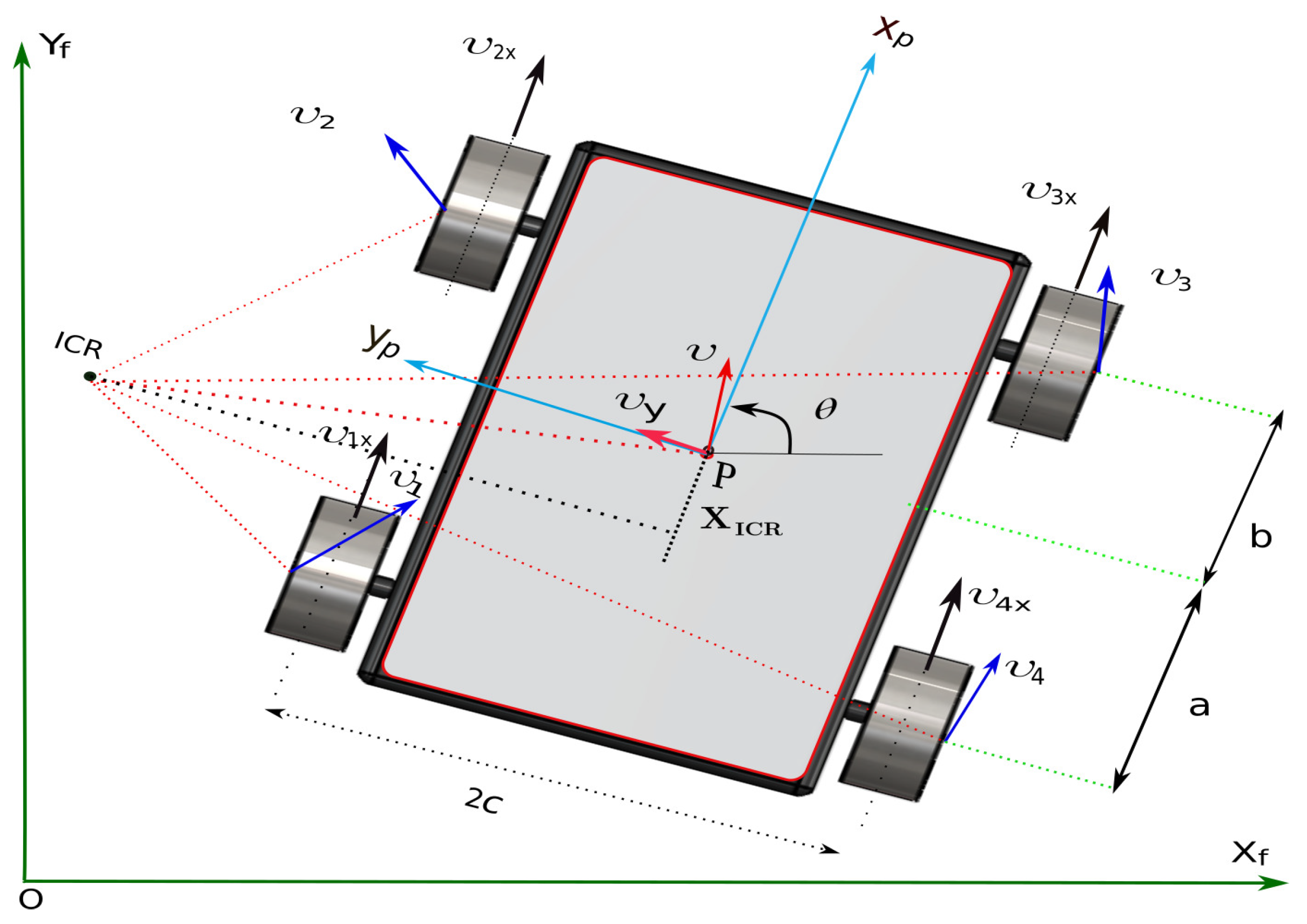
Another critical challenge SSMR faces is the change in the location of ICR during turning maneuvers due to lateral skidding. Depending on the location of ICR , the distance X ICR swings up and down along X-direction as shown in Figure 1. The nonlinear dynamic wheel-terrain interactions, instantaneous lateral velocity, and angular velocity during the curved path motion determine to what extent ICR shifts along the X-direction. The worst case scenario occurs if the X ICR extends beyond the robot wheelbase, which can skid laterally and lose motion stability. Incorporating such behavior into SSMR modeling is significantly challenging. Thus, most of the work carried out on SSMR ignores the effect of lateral skidding during turning maneuvers to simplify the modeling and control complexity. So far, however, very few studies have examined the role of lateral skidding, which commonly kept X ICR value to a constant value during turning maneuvers [8,12]. The varying nature of X ICR gives rise to alternations in model parameters, which calls for the need of a robust control method dealing with modeling uncertainties.
SMC is one of the most well-known robust control strategies that guarantee robust performance against uncertainties and disturbances. The design of an SMC contains two sequential steps that need to be undertaken. Primarily, a sliding manifold is formulated based on the desired error dynamics. Subsequently, the control input is designed to ensure that the system trajectories remain on the sliding manifold regardless of model uncertainties, nonlinearities and external disturbances [13,14,15]. An important feature of the linear sliding manifold is its simplicity, which guarantees asymptotic stability despite the slower convergence time of the states closer to equilibrium. That means the system states cannot reach the equilibrium in a finite time [15,16]. A terminal sliding mode control (TSMC) based on the nonlinear switching manifold has emerged to deal with this problem [16,17,18]. TSMC offers the benefit of a fast finite-time convergence of the states to equilibrium. As indicated by [18], however, uncertainties can potentially impact the robustness of TSMC. In addition, singularities may occur when the sliding manifold’s time derivative occurs, leading to infinite control input.
To tackle the singularity problem of TSMC, a nonsingular terminal sliding mode control (NTSMC) has been introduced in recent years. An adaptive fast NTSMC has been proposed by [19] to ensure precise and steady steering performance of a vehicle steer-by-wire system. The effectiveness of the NTSMC is verified via an experimental test, which shows a fast finite convergence and robust performance against different road conditions. [20] proposed a second-order fast NTSMC combined with ANN for rehabilitation robots to achieve a rapid convergence rate and robustness against uncertain parameters and disturbances, which ANN estimates. A cascaded NTSM-PID controller scheme has been presented in [21] to achieve robustness against disturbance and improve the tracking accuracy of a four-wheel independently driven skid steer robotic vehicle. In [17,22,23,24], NTSMC has also been designed for trajectory tracking control of robotic manipulators to obtain finite convergence of states to equilibrium and robust performance against uncertainties and external disturbances. In view of all that has been mentioned so far, some of the challenges associated with SSMR motion modeling and its control arise from the nonlinear behavior of coefficients of friction and change in the location of ICR, which pose modeling uncertainties. Therefore, well-calibrated robust control laws are needed to address these challenges so that SSMR can carry out its assigned tasks appropriately.
The main contributions of this paper are threefold: (a) This study formulated the uncertainties originating from friction forces due to wheel ground interaction, change in X ICR location, and external disturbances combined as lumped parametric uncertainties. Subsequently, an adaptive law is designed that tracks the occurrence uncertainties and estimates the lumped parametric uncertainties; (b) A continuous and chattering-free robust nonsingular terminal sliding mode control (NTSMC) based on a back-stepping method is developed; (c) In addition, the finite time stability of the closed-loop system is proven using Lyapunov’s theory.
The remainder of the paper is outlined as follows. Section 2 and Section 3 cover the kinematic and dynamic models of the SSMR, respectively. Section 4 proposes the formulation of robust control and the synthesis of finite-time stability. Section 5 presents some numerical simulation results. Finally, Section 6 gives some concluding remarks.

2. Kinematic Model

Typically, SSMR is equipped with wheels that cannot be steered, and it achieves steering by moving one side of the wheels at a faster speed than the other side [11,25]. As shown in Figure 1, two coordinate frames are defined to model the maneuverability of the SSMR: a fixed reference coordinate frame X f OY f , and a moving local coordinate frame attached at the robot’s center of mass (COM) as X p PY p . θ is the heading angle of the robot. The actual robot pose, q = [ X Y θ ] T , is used to define the robot’s configuration, while the reference (target) pose is represented by q ref , which defines q ref = [ X r e f Y r e f θ r e f ] T . Further details of SSMR modeling are found in [8,12]. If we define z as a displacement vector, then z ˙ = [ υ ω ] T , with υ and ω representing the velocity and angular velocity of the robot, respectively. υ i x and υ i y are the longitudinal and lateral velocities of the i t h wheel, respectively.
υ 1 x = υ 2 x = υ c ω υ 3 x = υ 4 x = υ + c ω υ 2 y = υ 3 y = ( X I C R + b ) ω υ 1 y = υ 4 y = ( X I C R a ) ω ,
where a , b , and c are the kinematic parameters of the SSMR shown in Figure 1.
A velocity constraint for SSMR was introduced in [12] as:
υ y + X ICR θ ˙ = 0 ,
where υ y is the lateral velocity.
It is essential to ensure the boundedness of X ICR to maintain lateral stability and reduce the robot’s sideslip angle during sharp turns [26]. The nonholonomic constraint can be rewritten in the Pfaffian form as follows:
[ sin θ cos θ X ICR ] [ X ˙ Y ˙ θ ˙ ] T = A ( q ) q ˙ = 0 .
If we let S ( q ) 3 × 2 be a full-rank matrix in which its columns are orthogonal to A ( q ) , then we can write:
S T ( q ) A T ( q ) = 0 ,
where S ( q ) is defined in the following equation.
S ( q ) = cos θ X ICR sin θ sin θ X ICR cos θ 0 1 .
Now, the generalized velocity vector can be written as:
q ˙ = S ( q ) z ˙ .
It has been noted from Equation (6) that the generalized velocity vector is dependent on X ICR . Differentiating both sides of Equation (6) leads to
q ¨ = S ( q ) z ¨ + S ˙ ( q ) z ˙ .

3. Dynamic Model

Lateral skidding is an inevitable phenomenon, and determining the exact location of the X ICR is difficult due to the nonlinear dynamic nature of the wheel-ground interaction during turning maneuvers. The unknown lateral skidding and ground interaction forces significantly affect the dynamic model of the SSMR. The dynamic model of the SSMR is formulated as [8]:
M ( q ) q ¨ + R ( q ˙ ) + A T ( q ) λ + τ d = B ( q ) τ .
where M ( q ) 3 × 3 , R ( q ˙ ) 3 × 1 , B ( q ) 3 × 2 , τ d 3 × 1 , τ 2 × 1 . Substituting Equation (7) into Equation (8) and multiplying both sides by S T yields:
M ˜ z ¨ + C ˜ z ˙ + R ˜ + τ ˜ d = B ˜ τ .
The terms M ˜ , C ˜ , R ˜ , τ ˜ d , and B ˜ are defined as follows:
M ˜ = S T MS = m 0 0 m X ICR 2 + I ,
C ˜ = S T M S ˙ = m X ICR 0 θ ˙ θ ˙ X ˙ ICR ,
R ˜ = S T R = F rx ( q ˙ ) X ICR F ry ( q ˙ ) + M r ,
τ ˜ d = S T τ d
B ˜ = S T B = 1 / r 1 1 c c ,
where m, I and r denote robot mass, moment of inertia, and wheel radius, respectively. It is important to note that M ˜ , C ˜ , and R ˜ , as defined earlier, are entirely dependent on the location of X ICR . Any change in the location of X ICR results in model parameter variations, thereby introducing model uncertainties to the dynamic system and poses a significant challenge in robot control.
F rx ( q ˙ ) , and F ry ( q ˙ ) represent the resistive forces in the inertial frame along the longitudinal and lateral directions, respectively, while M r ( q ˙ ) denotes the resistant moment around the center of mass. These forces and moments can be computed as follows [8]:
F rx ( q ˙ ) = m g μ x cos θ sgn v 2 x + sgn v 4 x 2 m g μ y sin θ a sgn v 3 y + b sgn v 4 y a + b .
F ry ( q ˙ ) = m g μ x sin θ sgn v 2 x + sgn v 4 x 2 + m g μ y cos θ a sgn v 3 y + b sgn v 4 y a + b .
M r ( q ˙ ) = m g 2 a b μ y sgn v 3 y 2 a b μ y sgn v 4 y 2 a + b m g a c μ x sgn v 2 x + a c μ x sgn v 4 x 2 a + b m g b c μ x sgn v 2 x + b c μ x sgn v 4 x 2 a + b ,
where g, μ x , and μ y represent the gravity of acceleration, longitudinal, and lateral coefficients of friction forces, respectively, sgn ( · ) denoting the signum function. Furthermore, it is essential to emphasize that the robot’s dynamic model of Equation (9) is also affected by model uncertainty due to the varying coefficients of friction forces, as denoted in Equations (10)–(12). These friction force coefficients depend primarily upon the dynamic nature of the surface of the wheel-ground interaction contact point.

4. Control Problem Formulation

For the trajectory tracking problem, the desired reference state vector is generated as follows.
q ˙ ref = X ˙ ref Y ˙ ref θ ˙ ref = cos θ 0 sin θ 0 0 1 υ ref ω ref .
where υ r e f and ω r e f are the reference velocity and angular velocity, respectively.
To ensure the robot pose to track the intended reference trajectory, the trajectory tracking error can be described in the following equation:
e = T ( θ ) ( q ref q ) ,
with e = [ e x e y e θ ] T , T ( θ ) is the transformation matrix that transforms the local into a fixed reference coordinate frame.
T ( θ ) = cos θ sin θ 0 sin θ cos θ 0 0 0 1 .
The corresponding tracking error derivative, e ˙ = [ e ˙ x e ˙ y e ˙ θ ] T , is thus readily obtained:
e ˙ x e ˙ y e ˙ θ = υ ref cos e θ υ ref sin e θ ω ref + 1 e y 0 e x 0 1 υ ω .
The popularity of the backstepping control approach has grown among researchers in recent decades due to its application to nonlinear systems. This approach systematically defines the Lyapunov function for stability analysis and the feedback control law design [27,28]. Moreover, it has the potential to be integrated with other control techniques, including neural networks [29], adaptive control [30], reinforcement learning [31], sliding mode control [32], and fuzzy control [33], to improve the system’s overall performance. By virtue of its distinctive advantages, the backstepping kinematic controller is proposed in this study to eliminate the pose tracking error, e . Subsequently, the control input, z ˙ c = [ υ c ω c ] T , can also be used as a command velocity to NTSMC. As proposed by [34], z ˙ c can be given by
υ c ω c = k x e x + υ ref cos e θ ω ref + k y υ ref e y + k θ υ ref sin e θ ,
where k x , k y , k θ are positive constant numbers.
Assuming that υ r e f and ω r e f are constant, the time derivative of z ˙ c can be determined as [35]:
υ ˙ c ω ˙ c = k x e ˙ x υ ref e ˙ θ sin e θ k y υ ref e ˙ y + k θ υ ref e ˙ θ cos e θ .
Definition 1. 
If we define the signal e z = z c z , the velocity tracking error, e ˙ z , can be defined as the difference between the command velocity control inputs z ˙ c and the true velocity z ˙ .
e ˙ z = z ˙ c z ˙ .
with e ˙ z = [ e ˙ z 1 e ˙ z 2 ] T
It has been well-known that the coefficient of friction is highly nonlinear, complex, and difficult to model. Furthermore, accurately determining the X ICR while executing a turning maneuver poses a considerable challenge. The dynamic equation of Equation (9) can be rewritten as
( M ˜ 0 + Δ M ˜ ) z ¨ + ( C ˜ 0 + Δ C ˜ ) z ˙ + ( R ˜ 0 + Δ R ˜ ) + τ ˜ d = B ˜ τ ,
where M ˜ 0 , C ˜ 0 and R ˜ 0 denote the nominal model parameters and Δ M ˜ , Δ C ˜ and Δ R ˜ are the corresponding uncertainties. If we define the lumped parametric uncertainties as ρ = Δ M ˜ z ¨ + Δ C ˜ z ˙ + Δ R ˜ + τ ˜ d , then Equation (20) can be written as:
M ˜ 0 z ¨ + C ˜ 0 z ˙ + R ˜ 0 = B ˜ τ ρ ,
The parametric uncertainties are upper bound by positive vectors b 0 and b 1 but are assumed to be unknown.
ρ b 0 + z ˙ ρ b 1 ,
where z ˙ ρ = diag ( υ , ω ) , b 0 = [ b 01 b 02 ] T , b 1 = [ b 11 b 12 ] T .
Taking the time derivative of Equation (19) and using Equation (21) yields the error dynamics as follows:
e ¨ z = z ¨ c M ˜ 0 1 ( B ˜ τ ρ C ˜ 0 z ˙ R ˜ 0 ) .
As discussed above, a nonsingular terminal sliding manifold is selected to avoid the singularity problem [16] as
S = β e z + e ˙ z γ sgn ( e ˙ z ) ,
where S = [ S 1 S 2 ] T , β = diag ( β 1 , β 2 ) , e ˙ z γ sgn ( e ˙ z ) = [ e ˙ z 1 γ 1 sgn ( e ˙ z 1 ) e ˙ z 2 γ 2 sgn ( e ˙ z 2 ) ] T , and β i > 0 , 1 < γ i < 2 for i = 1, 2.
To ensure the sliding motion occurs, the derivative of sliding surface S ˙ = 0 should be satisfied.
S ˙ = β e ˙ z + γ e ˙ z γ 1 e ¨ z ,
where γ e ˙ z γ 1 = diag ( γ 1 e ˙ z γ 1 1 , γ 2 e ˙ z γ 2 1 )
For the tracking problem, substituting Equation (23) into Equation (25) leads to
S ˙ = β e ˙ z + γ e ˙ z γ 1 [ z ¨ c M ˜ 0 1 ( B ˜ τ ρ C ˜ 0 z ˙ R ˜ 0 ) ] .
The design of feedback control is vital to stabilize S = 0 to ensure the attractive property of the manifold. According to the sliding mode control design, the control input can be defined as
τ = τ eq + τ r ,
where τ eq is the equivalent control and τ r is reaching control to ensure the reachability of the sliding manifold. τ eq can be obtained by setting S ˙ = 0 and ρ = 0 .
τ eq = ( M ˜ 0 1 B ˜ ) 1 [ β γ 1 e ˙ z 2 γ sgn ( e ˙ z ) + z ¨ c + M ˜ 0 1 C ˜ 0 z ˙ + M ˜ 0 1 R ˜ 0 ] .
Referring to Equation (22), let b ^ i be the estimation of upper bound, and b i the true upper bound assuming that b ^ i b i , for i = 0 , 1 . The reaching control, τ r , can be designed as [36]
τ r = ( M ˜ 0 1 B ˜ ) 1 [ k 1 S + k 2 S σ sgn ( S ) + ( b ^ 0 + z ˙ ρ b ^ 1 ) ] ,
where k 1 = diag ( k 11 , k 12 ) , k 2 = diag ( k 21 , k 22 ) , S σ sgn ( S ) = [ S 1 σ 1 sgn ( S 1 ) S 2 σ 2 sgn ( S 2 ) ] T , and k 1 i , k 2 i > 0 and 0 < σ i < 1 for i=0,1. Therefore, the total NTSMC law for the system is given by:
τ = ( M ˜ 0 1 B ˜ ) 1 [ β γ 1 e ˙ z 2 γ sgn ( e ˙ z ) + z ¨ c + M ˜ 0 1 C ˜ 0 z ˙ + M ˜ 0 1 R ˜ 0 + k 1 S + k 2 S σ sgn ( S ) + ( b ^ 0 + z ˙ ρ b ^ 1 ) ] .
The S ˙ of Equation (26) is simplified further by substituting Equation (30) into Equation (26).
S ˙ = γ e ˙ z γ 1 [ k 1 S k 2 S σ sgn ( S ) + ( b ¯ 0 + z ˙ ρ b ¯ 1 ) ] ,
where b ¯ 0 and b ¯ 1 are defined as b ¯ 0 = b ^ 0 b 0 and b ¯ 1 = b ^ 1 b 1 .
If ψ = [ S b ¯ 0 b ¯ 1 ] T is defined as the state vector, then the Lyapunov function V ( ψ ) is expressed as:
V ( ψ ) = 1 2 S T S + 1 2 α 0 b ¯ 0 T b ¯ 0 + 1 2 α 1 b ¯ 1 T b ¯ 1 ,
where α 0 and α 1 are positive constants. The time derivative of V ( ψ ) yields
V ˙ = S T S ˙ + α 0 b ^ ˙ 0 T b ¯ 0 + α 1 b ^ ˙ 1 T b ¯ 1 .
Substituting Equation (31) into Equation (33) yields,
V ˙ = S T ( γ e ˙ z γ 1 [ k 1 S k 2 S σ sgn ( S ) + ( b ¯ 0 + z ˙ ρ b ¯ 1 ) ] ) + α 0 b ^ ˙ 0 T b ¯ 0 + α 1 b ^ ˙ 1 T b ¯ 1 .
Rearranging Equation (34) gives
V ˙ = S T γ e ˙ z γ 1 k 1 S S T γ e ˙ z γ 1 k 2 S σ sgn ( S ) + S T γ e ˙ z γ 1 b ¯ 0 + S T γ e ˙ z γ 1 z ˙ ρ b ¯ 1 + α 0 b ^ ˙ 0 T b ¯ 0 + α 1 b ^ ˙ 1 T b ¯ 1 .
The following inequality holds since S T γ e ˙ z γ 1 k 2 S σ sgn ( S ) 0 . In addition, the assumption b ^ i b i leads to b ¯ i 0 .
V ˙ S T γ e ˙ z γ 1 k 1 S + S T γ e ˙ z γ 1 b ¯ 0 + S T γ e ˙ z γ 1 z ˙ ρ b ¯ 1 + α 0 b ^ ˙ 0 T b ¯ 0 + α 1 b ^ ˙ 1 T b ¯ 1 = S T γ e ˙ z γ 1 k 1 S S T γ e ˙ z γ 1 b ¯ 0 S T γ e ˙ z γ 1 z ˙ ρ b ¯ 1 2 α 0 b ^ ˙ 0 T b ¯ 0 + α 0 b ^ ˙ 0 T b ¯ 0 2 α 1 b ^ ˙ 1 T b ¯ 1 + α 1 b ^ ˙ 1 T b ¯ 1 ,
where b ¯ 0 = [ b ¯ 01 b ¯ 02 ] T and b ¯ 1 = [ b ¯ 11 b ¯ 12 ] T . We know that b ^ i is assumed to be positive. In order to develop an adaptive law to estimate the lumped parametric uncertainties, Equation (36) can be written as
V ˙ S T γ e ˙ z γ 1 k 1 S + ( α 0 b ^ ˙ 0 T S T γ e ˙ z γ 1 ) b ¯ 0 + ( α 1 b ^ ˙ 1 T S T γ e ˙ z γ 1 z ˙ ρ ) b ¯ 1 2 α 0 b ^ ˙ 0 T b ¯ 0 2 α 1 b ^ ˙ 1 T b ¯ 1 ,
where S T = [ S 1 S 2 ] . Therefore, the estimation adaptive law of b ^ ˙ 0 and b ^ ˙ 1 can be explicitly defined as: b ^ ˙ 0 = [ b ^ ˙ 01 b ^ ˙ 02 ] T and b ^ ˙ 1 = [ b ^ ˙ 11 b ^ ˙ 12 ] T . Note: γ 01 = γ 11 = γ 1 and γ 02 = γ 12 = γ 2 . Similarly, α 01 = α 02 = α 0 and α 11 = α 12 = α 1 . Thus, the estimation update rule becomes,
b ^ ˙ 01 = γ 01 α 01 s 1 υ c υ γ 01 1 .
b ^ ˙ 02 = γ 02 α 02 s 2 ω c ω γ 02 1 .
b ^ ˙ 11 = γ 11 α 11 s 1 υ c υ γ 11 1 υ .
b ^ ˙ 12 = γ 12 α 12 s 2 ω c ω γ 12 1 ω .
Now, Equation (37) is simplified as
V ˙ S T γ e ˙ z γ 1 k 1 S 2 α 0 b ^ ˙ 0 T b ¯ 0 2 α 1 b ^ ˙ 1 T b ¯ 1 = ( S T γ e ˙ z γ 1 k 1 S + 2 α 0 b ^ ˙ 0 T b ¯ 0 + 2 α 1 b ^ ˙ 1 T b ¯ 1 ) .
Substituting Equations (38)–(4) into Equation (42) yields,
V ˙ ( γ 1 k 11 υ c υ γ 1 1 s 1 s 1 + γ 2 k 12 ω c ω γ 2 1 s 2 s 2 + 2 γ 01 α 01 α 01 s 1 υ c υ γ 01 1 b ¯ 01 + 2 γ 02 α 02 α 02 s 2 ω c ω γ 02 1 b ¯ 02 + 2 γ 11 α 11 α 11 s 1 υ c υ γ 11 1 υ b ¯ 11 + 2 γ 12 α 12 α 12 s 2 ω c ω γ 12 1 ω b ¯ 12 ) .
To achieve a more concise expression, we define that: Γ 1 = γ 1 k 01 υ c υ γ 1 1 s 1 ,
Γ 2 = γ 2 k 02 ω c ω γ 2 1 s 2 ,
Γ 3 = 2 γ 01 α 01 υ c υ γ 01 1 s 1 ,
Γ 4 = 2 γ 02 α 02 ω c ω γ 02 1 s 2 ,
Γ 5 = 2 γ 11 α 11 υ c υ γ 12 1 s 1 υ ,
Γ 6 = 2 γ 12 α 12 ω c ω γ 12 1 s 2 ω
Now, V ˙ is rewritten as
V ˙ ( Γ 1 s 1 + Γ 2 s 2 + Γ 3 α 01 b ¯ 01 + Γ 4 α 02 b ¯ 02 + Γ 5 α 11 b ¯ 11 + Γ 6 α 12 b ¯ 12 ) η ( s 1 + s 2 + α 01 b ¯ 01 + α 02 b ¯ 02 + α 11 b ¯ 11 + α 12 b ¯ 12 ) ,
where η = min Γ 1 , Γ 2 , Γ 3 , Γ 4 , Γ 5 , Γ 6 .
It is noteworthy that the subsequent inequality is valid [37] for X , Y , Z :
( X 2 + Y 2 + Z 2 ) 1 2 X + Y + Z .
Hence, Equation (44) is simplified as
V ˙ 2 η V 1 2 .
Lemma 1 
([38,39]). Consider the nonlinear system described by ξ ˙ = f ( ξ ) , whose equilibrium is ξ = 0 . Suppose there is a C 1 (continuously differentiable) function V ( x ) defined in a neighborhood D n of the origin, and there are real numbers Υ > 0 and 0 < φ < 1 , such that V ( x ) > 0 on D and V ˙ ( x ) + Υ V φ ( x ) 0 (along the trajectory) on D. Then the origin of the system is finite-time stable. Moreover, the settling time, depending on the initial slate x ( 0 ) = x o , is given by
T ( x o ) 1 Υ ( 1 φ ) V 1 φ ( x o ) ,
for x o in some open neighborhood of the origin.
Hence, the finite-time stability criterion of the system is satisfied based on Lemma 1, implying that V converges from initial V ( 0 ) to the origin according to the inequality given by Equation (46).
T ( 0 ) 2 2 η V 1 2 ( 0 ) .
Despite uncertainties and disturbances, the sliding surface S , b ¯ 0 , and b ¯ 1 will converge to the origin within finite time T ( 0 ) .

5. Numerical Results

The numerical example is used to implement the proposed control strategy. The SSMR is required to follow a desired circular trajectory path starting from an initial pose of q ( 0 ) = [ 2.0 1.0 pi / 4 ] T . The reference circular trajectory is defined in Equation (13), where the reference velocities are given by υ r e f = 0.5 m / s and ω r e f = 0.2 r a d / s . The design parameters were chosen from [12] to represent a typical SSMR. Referring to Figure 1, the dimensions of the SSMR are given as: a = 0.55 m , b = 0.37 m , 2 c = 0.63 m , and the wheel radius is r = 0.2 m . Additionally, the mass and inertia of SSMR are m = 116 kg , and I = 20 kgm 2 , respectively. The nominal friction coefficients for lateral and longitudinal direction are μ y 0 = 0.35 and μ x 0 = 0.15 , respectively. As noted in [8], a fixed coordinate of the ICR should be selected as X ICR ( a , b ) . Hence, the nominal X ICR 0 is selected as 0.18 m .
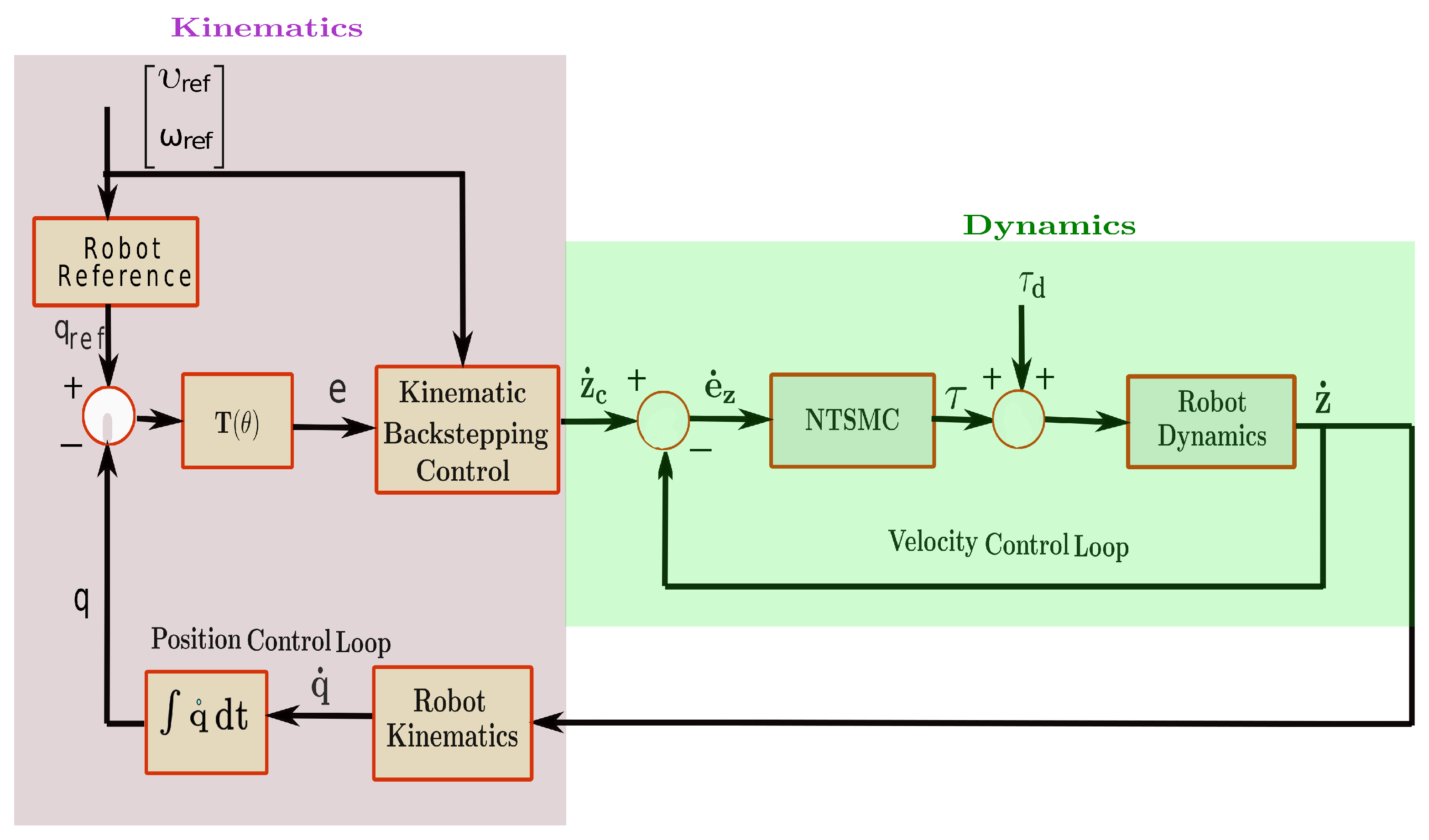
The complete control diagram of the wheeled mobile robot is shown in Figure 2. It has been noted that the parametric change in X ICR has introduced parametric uncertainties in M ˜ , C ˜ and R ˜ . Moreover, the parametric change in the coefficient of friction has introduced parametric uncertainties in R ˜ . In order to validate the performance of robustness against modeling uncertainties, the following uncertainties are considered: δ μ x = 0.15 sin ( π / 4 ) for t 10 s , δ μ y = 0.2 sin ( π / 4 ) for 15 t 20 s , δ X ICR = 0.09 sin ( π / 4 ) for 25 t 30 s and δ τ d = 35 sin ( π / 4 ) for 35 t 45 s . The constant gains undergo tuning in various simulation tests, and the final values are provided as: k x = 1.5 , k y = 20.5 , k θ = 2.5 , α 0 = α 1 = 22 , β = [ 2.4 2.4 ] T , γ = [ 1.5 1.5 ] T , k 1 = [ 4.5 4.5 ] , k 2 = [ 20 20 ] , σ = [ 0.5 0.5 ] T .
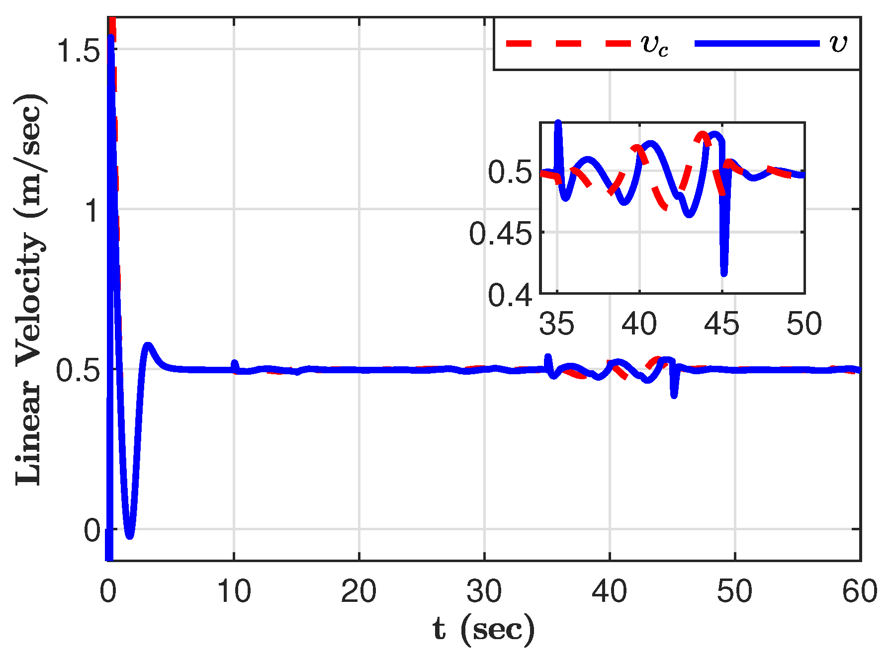
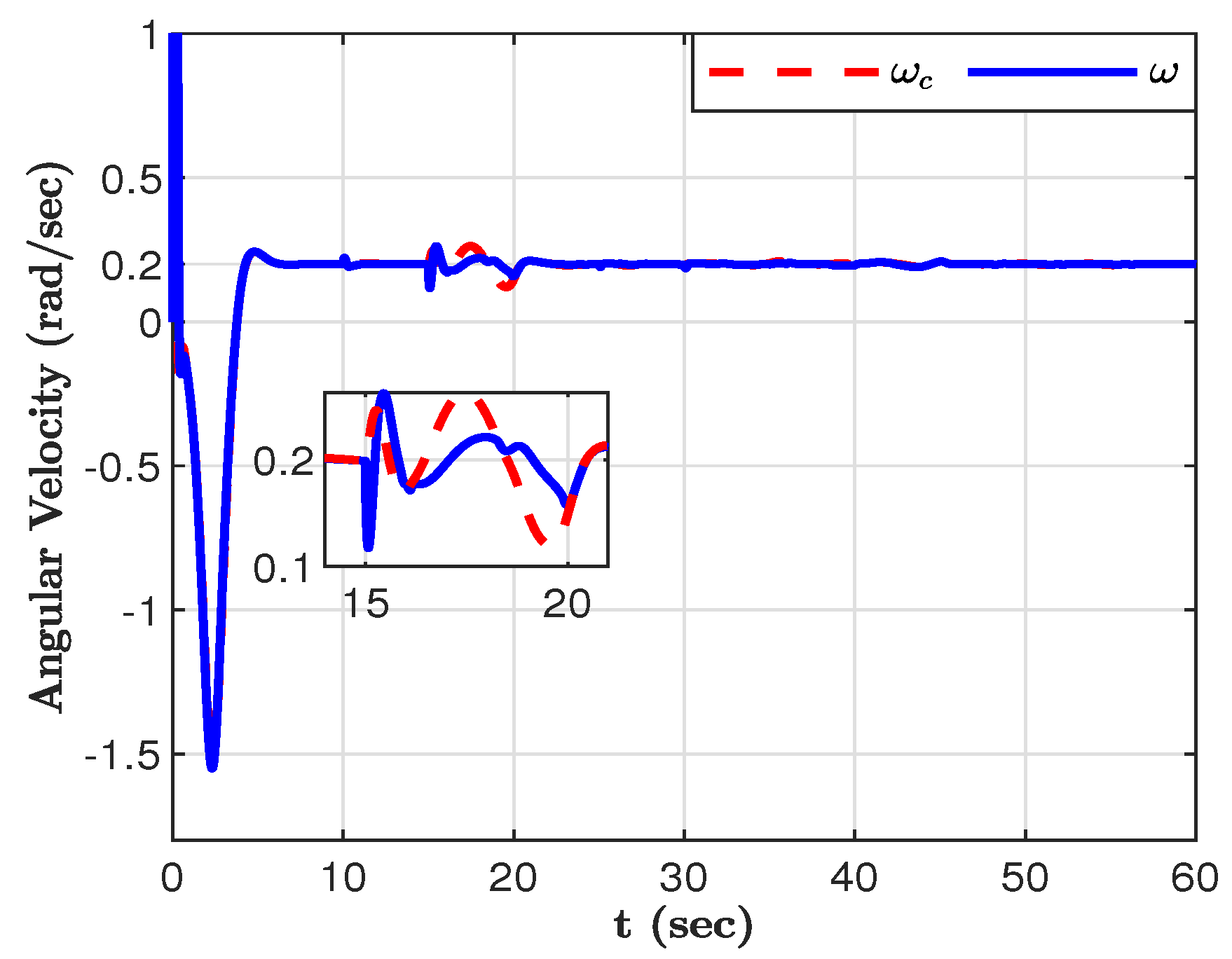
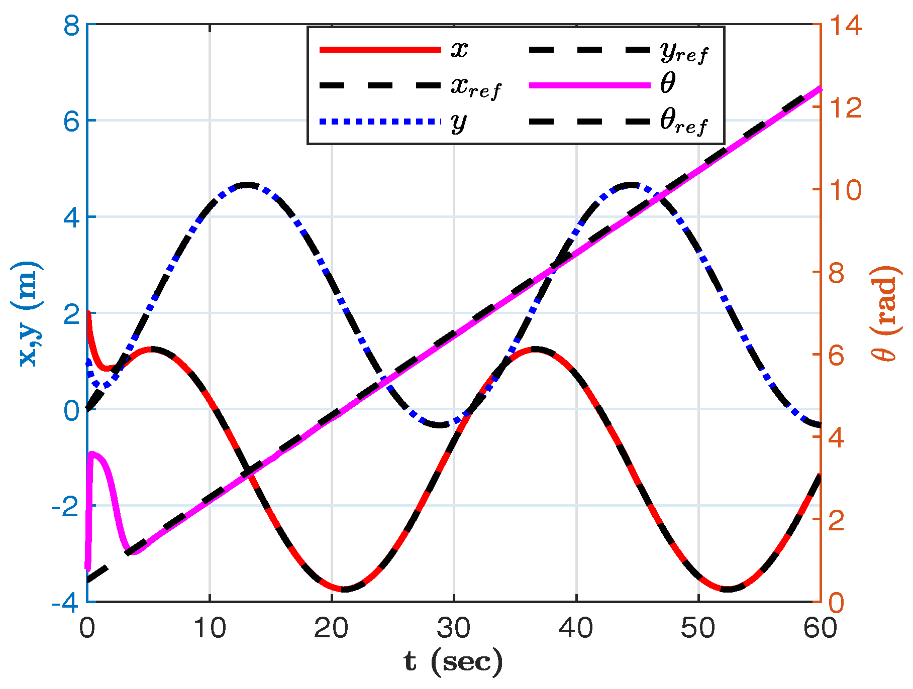
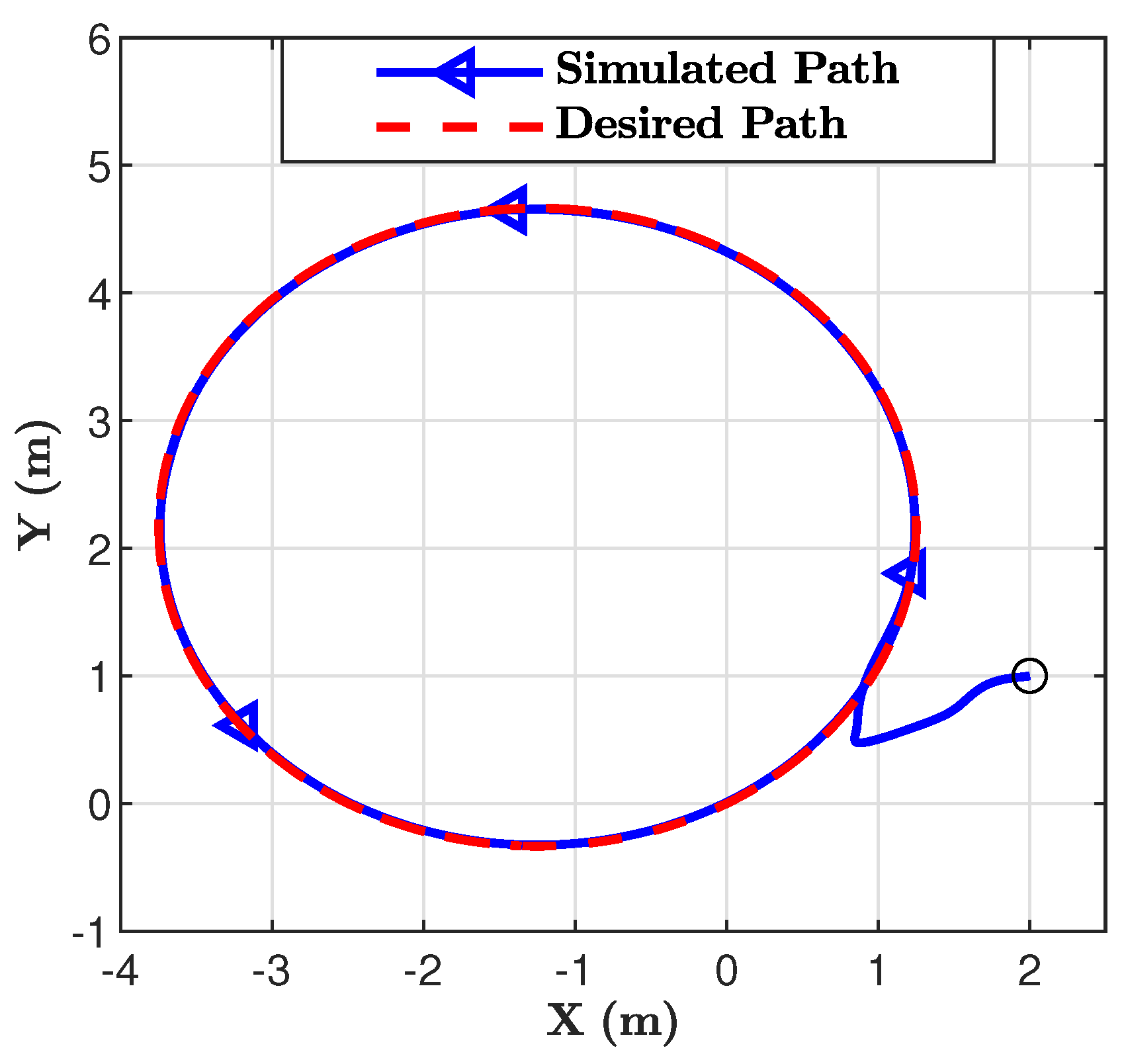
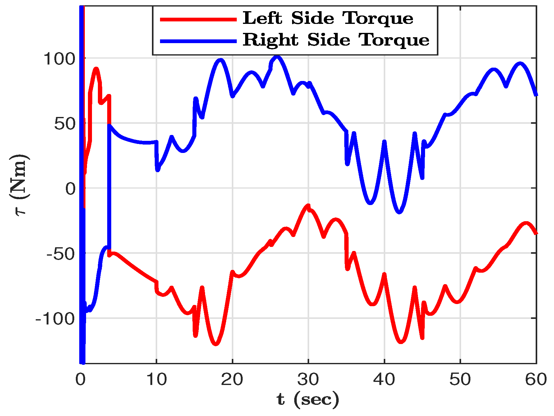
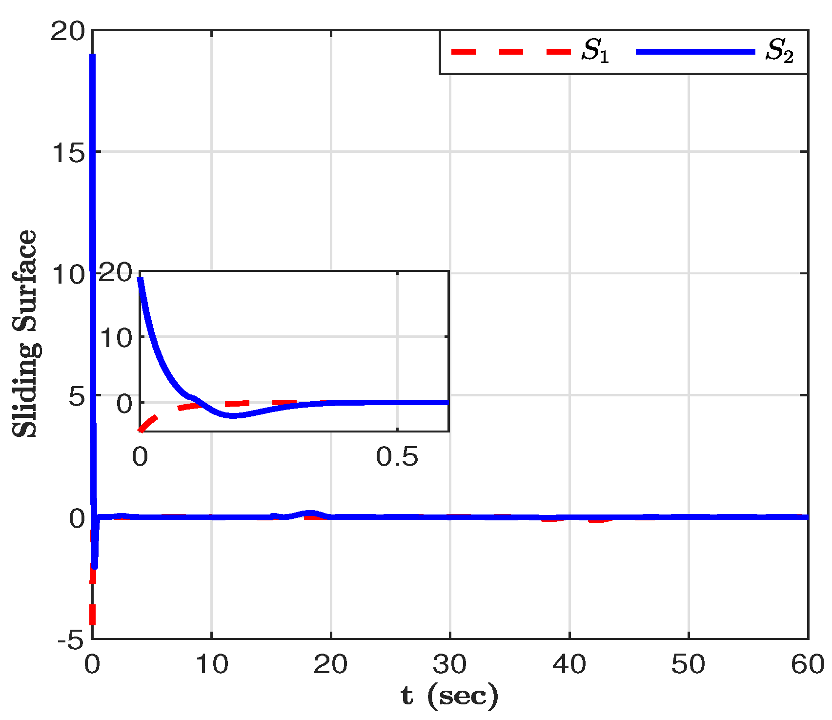
The robustness of NTSMC against model uncertainties and external disturbances is examined by considering time-varying parametric perturbation of X ICR , friction coefficients along the x and y directions during turning maneuvers. Figure 3 and Figure 4 illustrate the time history of the velocity and angular velocity of the SSMR, respectively. It is clear that the velocity does not converge near the initial time, which denotes unstable motion; however, it is stabilized for the rest of the simulation time. Compared to other types of uncertainties, the external disturbance has a notable effect on velocity, as shown in Figure 3. On the other hand, disturbance in lateral friction force has a notable influence on the angular velocity of the robot, as shown in Figure 4. However, as shown in the time history of the figures, the designed NTSMC eliminates both disturbances and performs better trajectory tracking. The robot poses are plotted in Figure 5, which shows the SSMR accurately tracks the target pose despite the disturbances. As shown in Figure 6, the robot follows the desired circular path precisely in spite of the disturbances. Figure 7 shows that the proposed torque input is a continuous control and does not exhibit a noticeable chattering problem. It has been observed from the simulation results that time-varying parametric perturbation of X I C R during turning maneuvers is successfully compensated by robust NTSMC. Finally, the simulation results shown in Figure 8 clearly reveal the asymptotically convergent property of NTSMC.
6. Conclusions

Accurately determining uncertainties caused by changes in ICR location, friction force, and external disturbances poses a significant challenge. The proposed control strategy generally comprises the position control loop using the backstepping technique and the velocity control loop using NTSMC to eliminate the position and velocity errors, respectively. The Lyapunov function has been used to obtain the lumped parametric uncertainties, and the finite-time stability of the overall system has also been verified. Circular trajectory path simulations for typical SSMR are conducted to verify the proposed approach. The proposed sliding surfaces converge to the origin despite the uncertainties and disturbances, which demonstrates that the control strategy is robust against modeling uncertainties and disturbances. In addition, the simulation result validates that NTSMC is chattering and singularity-free control. Notably, the structure and parameter of lumped uncertainties are predefined in the proposed method. In the future, a more flexible non-parametric learning-based uncertainty prediction will be investigated to achieve adjustable parameters for lumped uncertainties by conducting experiments on SSMRs.

Author Contributions

Mulugeta Debebe Teji is responsible for the basic concepts, discussing the results, and writing the article. Ting Zou is the corresponding author, responsible for the basic concepts, discussing the results, proofreading, and revising the manuscript. Dinku Seyoum Zeleke is responsible for proofreading and revising the manuscript. All authors read and approved the final manuscript.

Funding

This research received no external funding.

Institutional Review Board Statement

Not applicable.

Informed Consent Statement

Not applicable.

Data Availability Statement

Not applicable.

Conflicts of Interest

The authors declare no conflicts of interest.

References

  1. Emmi, L.; Fernández, R.; Gonzalez-de Santos, P. An efficient guiding manager for ground mobile robots in agriculture. Robotics 2023, 13, 6. [Google Scholar] [CrossRef]
  2. Jun, J.Y.; Hua, M.D.; Benamar, F. A trajectory tracking control design for a skid-steering mobile robot by adapting its desired instantaneous center of rotation. 53rd IEEE Conference on Decision and Control. IEEE, 2014, pp. 4554–4559.
  3. Ostafew, C.J.; Schoellig, A.P.; Barfoot, T.D. Learning-based nonlinear model predictive control to improve vision-based mobile robot path-tracking in challenging outdoor environments. 2014 IEEE International Conference on Robotics and Automation (ICRA). IEEE, 2014, pp. 4029–4036.
  4. Srikonda, S.; Norris, W.R.; Nottage, D.; Soylemezoglu, A. Deep Reinforcement Learning for Autonomous Dynamic Skid Steer Vehicle Trajectory Tracking. Robotics 2022, 11, 95. [Google Scholar] [CrossRef]
  5. Juman, M.A.; Wong, Y.W.; Rajkumar, R.K.; Kow, K.W.; Yap, Z.W. An incremental unsupervised learning based trajectory controller for a 4 wheeled skid steer mobile robot. Engineering Applications of Artificial Intelligence 2019, 85, 385–392. [Google Scholar] [CrossRef]
  6. Zhu, C.W.; Hill, E.; Biglarbegian, M.; Gadsden, S.A.; Cline, J.A. Smart agriculture: Development of a skid-steer autonomous robot with advanced model predictive controllers. Robotics and Autonomous Systems 2023, 162, 104364. [Google Scholar]
  7. Yi, J.; Song, D.; Zhang, J.; Goodwin, Z. Adaptive trajectory tracking control of skid-steered mobile robots. Proceedings 2007 IEEE International Conference on Robotics and Automation. IEEE, 2007, pp. 2605–2610.
  8. Kozłowski, K.; Pazderski, D. Modeling and control of a 4-wheel skid-steering mobile robot. International journal of applied mathematics and computer science 2004, 14, 477–496. [Google Scholar]
  9. Prado, A.J.; Torres-Torriti, M.; Cheein, F.A. Distributed tube-based nonlinear MPC for motion control of skid-steer robots with terra-mechanical constraints. IEEE Robotics and Automation Letters 2021, 6, 8045–8052. [Google Scholar] [CrossRef]
  10. Prado, Á.J.; Torres-Torriti, M.; Yuz, J.; Cheein, F.A. Tube-based nonlinear model predictive control for autonomous skid-steer mobile robots with tire–terrain interactions. Control Engineering Practice 2020, 101, 104451. [Google Scholar] [CrossRef]
  11. Yue, X.; Chen, J.; Li, Y.; Zou, R.; Sun, Z.; Cao, X.; Zhang, S. Path tracking control of skid-steered mobile robot on the slope based on fuzzy system and model predictive Control. International Journal of Control, Automation and Systems 2022, 20, 1365–1376. [Google Scholar] [CrossRef]
  12. Caracciolo, L.; De Luca, A.; Iannitti, S. Trajectory tracking control of a four-wheel differentially driven mobile robot. Proceedings 1999 IEEE international conference on robotics and automation (Cat. No. 99CH36288C). IEEE, 1999, Vol. 4, pp. 2632–2638.
  13. Slotine, J.J.E.; Li, W.; others, *!!! REPLACE !!!*. Applied nonlinear control; Prentice hall Englewood Cliffs: NJ, 1991; Volume 199. [Google Scholar]
  14. Edwards, C.; Spurgeon, S. Sliding mode control: Theory and applications; Crc Press, 1998. [Google Scholar]
  15. Wang, X.; van Kampen, E.J.; Chu, Q. Quadrotor fault-tolerant incremental nonsingular terminal sliding mode control. Aerospace Science and Technology 2019, 95, 105514. [Google Scholar] [CrossRef]
  16. Yu, X.; Feng, Y.; Man, Z. Terminal sliding mode control–an overview. IEEE Open Journal of the Industrial Electronics Society 2020, 2, 36–52. [Google Scholar] [CrossRef]
  17. Feng, Y.; Yu, X.; Man, Z. Non-singular terminal sliding mode control of rigid manipulators. Automatica 2002, 38, 2159–2167. [Google Scholar] [CrossRef]
  18. Wu, Y.; Yu, X.; Man, Z. Terminal sliding mode control design for uncertain dynamic systems. Systems & Control Letters 1998, 34, 281–287. [Google Scholar]
  19. Sun, Z.; Zheng, J.; Wang, H.; Man, Z. Adaptive fast non-singular terminal sliding mode control for a vehicle steer-by-wire system. IET Control Theory & Applications 2017, 11, 1245–1254. [Google Scholar]
  20. Liang, X.; Wang, H.; Zhang, Y. Adaptive nonsingular terminal sliding mode control for rehabilitation robots. Computers and Electrical Engineering 2022, 99, 107718. [Google Scholar] [CrossRef]
  21. Xiong, R.; Li, L.; Zhang, C.; Ma, K.; Yi, X.; Zeng, H. Path tracking of a four-wheel independently driven skid steer robotic vehicle through a cascaded ntsm-pid control method. IEEE Transactions on Instrumentation and Measurement 2022, 71, 1–11. [Google Scholar] [CrossRef]
  22. Yi, S.; Zhai, J. Adaptive second-order fast nonsingular terminal sliding mode control for robotic manipulators. ISA transactions 2019, 90, 41–51. [Google Scholar] [CrossRef]
  23. Zhai, J.; Xu, G. A novel non-singular terminal sliding mode trajectory tracking control for robotic manipulators. IEEE Transactions on Circuits and Systems II: Express Briefs 2020, 68, 391–395. [Google Scholar] [CrossRef]
  24. Choi, J.; Baek, J.; Lee, W.; Lee, Y.S.; Han, S. Adaptive model-free control with nonsingular terminal sliding-mode for application to robot manipulators. IEEE Access 2020, 8, 169897–169907. [Google Scholar] [CrossRef]
  25. Huskić, G.; Buck, S.; Herrb, M.; Lacroix, S.; Zell, A. High-speed path following control of skid-steered vehicles. The International Journal of Robotics Research 2019, 38, 1124–1148. [Google Scholar] [CrossRef]
  26. Flögel, D.; Bhatt, N.P.; Hashemi, E. Infrastructure-aided localization and state estimation for autonomous mobile robots. Robotics 2022, 11, 82. [Google Scholar] [CrossRef]
  27. Hacioglu, Y.; Yagiz, N. Fuzzy robust backstepping with estimation for the control of a robot manipulator. Transactions of the Institute of Measurement and Control 2019, 41, 2816–2825. [Google Scholar] [CrossRef]
  28. Krstic, M.; Kokotovic, P.V.; Kanellakopoulos, I. Nonlinear and adaptive control design; John Wiley & Sons, Inc., 1995. [Google Scholar]
  29. Luo, Y.; Zhao, S.; Yang, D.; Zhang, H. A new robust adaptive neural network backstepping control for single machine infinite power system with TCSC. IEEE/CAA Journal of Automatica Sinica 2019, 7, 48–56. [Google Scholar] [CrossRef]
  30. Caiazzo, B.; Lui, D.G.; Petrillo, A.; Santini, S. Resilient adaptive finite-time fault-tolerant control for heterogeneous uncertain and nonlinear autonomous connected vehicles platoons. IEEE Open Journal of Intelligent Transportation Systems 2023. [Google Scholar] [CrossRef]
  31. Lin, Y.C.; Nguyen, H.L.T.; Yang, J.F.; Chiou, H.J. A reinforcement learning backstepping-based control design for a full vehicle active Macpherson suspension system. IET Control Theory & Applications 2022, 16, 1417–1430. [Google Scholar]
  32. Alipour, M.; Zarei, J.; Razavi-Far, R.; Saif, M.; Mijatovic, N.; Dragičević, T. Observer-based backstepping sliding mode control design for microgrids feeding a constant power load. IEEE Transactions on Industrial Electronics 2022, 70, 465–473. [Google Scholar] [CrossRef]
  33. Wu, X.; Jin, P.; Zou, T.; Qi, Z.; Xiao, H.; Lou, P. Backstepping trajectory tracking based on fuzzy sliding mode control for differential mobile robots. Journal of Intelligent & Robotic Systems 2019, 96, 109–121. [Google Scholar]
  34. Kanayama, Y.; Kimura, Y.; Miyazaki, F.; Noguchi, T. A stable tracking control method for an autonomous mobile robot. Proceedings., IEEE International Conference on Robotics and Automation. IEEE, 1990, pp. 384–389.
  35. Zou, T.; Angeles, J.; Hassani, F. Dynamic modeling and trajectory tracking control of unmanned tracked vehicles. Robotics and Autonomous Systems 2018, 110, 102–111. [Google Scholar] [CrossRef]
  36. Xie, H.; Zheng, J.; Sun, Z.; Wang, H.; Chai, R. Finite-time tracking control for nonholonomic wheeled mobile robot using adaptive fast nonsingular terminal sliding mode. Nonlinear Dynamics 2022, 110, 1437–1453. [Google Scholar] [CrossRef]
  37. Zhou, Z.; Tang, G.; Xu, R.; Han, L.; Cheng, M. A novel continuous nonsingular finite–time control for underwater robot manipulators. Journal of Marine Science and Engineering 2021, 9, 269. [Google Scholar] [CrossRef]
  38. Hong, Y.; Huang, J.; Xu, Y. On an output feedback finite-time stabilization problem. IEEE transactions on Automatic Control 2001, 46, 305–309. [Google Scholar] [CrossRef]
  39. Yu, S.; Yu, X.; Shirinzadeh, B.; Man, Z. Continuous finite-time control for robotic manipulators with terminal sliding mode. Automatica 2005, 41, 1957–1964. [Google Scholar] [CrossRef]
Figure 1. Skid-steered wheeled mobile robot.
Preprints 137489 g001
Figure 2. The overall structure of the proposed control scheme.
Preprints 137489 g002
Figure 3. Velocity of the robot.
Preprints 137489 g003
Figure 4. Angular velocity of the robot.
Preprints 137489 g004
Figure 5. Pose of the robot.
Preprints 137489 g005
Figure 6. Robot following a desired circular path.
Preprints 137489 g006
Figure 7. Torque input.
Preprints 137489 g007
Figure 8. Sliding surface.
Preprints 137489 g008
Disclaimer/Publisher’s Note: The statements, opinions and data contained in all publications are solely those of the individual author(s) and contributor(s) and not of MDPI and/or the editor(s). MDPI and/or the editor(s) disclaim responsibility for any injury to people or property resulting from any ideas, methods, instructions or products referred to in the content.
Copyright: This open access article is published under a Creative Commons CC BY 4.0 license, which permit the free download, distribution, and reuse, provided that the author and preprint are cited in any reuse.
Alerts
Prerpints.org logo

Preprints.org is a free preprint server supported by MDPI in Basel, Switzerland.

Subscribe

© 2025 MDPI (Basel, Switzerland) unless otherwise stated