
Submitted:
29 October 2024
Posted:
30 October 2024
You are already at the latest version
Abstract
Ventilation, cooling, and heating systems play a crucial role in providing thermal comfort within occupied environments, influencing productivity, well-being, health, and energy consumption. This research focuses on leveraging Computational Fluid Dynamics (CFD) as a tool for studying fluid flows and analyzing heating, ventilation, and air conditioning (HVAC) systems to achieve ideal room temperatures efficiently. Initially, the thermal comfort study is conducted using the OpenFOAM software, aiming to compare and validate its algorithm against a reference article that utilized proprietary software. By demonstrating the capabilities of OpenFOAM as an open-source alternative, this research opens opportunities for analyzing HVAC systems using an accessible program, facilitating the optimization of climatization strategies. Subsequently, an analysis of ventilation systems is performed through a factorial design that involves altering the positions of air inlets and outlets, as well as adjusting the insufflation velocity. The findings reveal that superior positions of air inlets lead to improved thermal comfort results, as measured by the Air Diffusion Performance Index (ADPI). This research provides an insights in the configuration of ventilation and air conditioning systems to enhance occupant’s thermal comfort. By utilizing CFD simulations and exploring several parameters affecting thermal comfort, this research contributes to advancing HVAC system analysis.
Keywords:
Computational Fluid Dynamics
; Thermal Comfort
; HVAC Systems
; OpenFOAM
; Factorial Design
1. Introduction
The design and construction of buildings are driven by the aspiration to create environments that offer comfort and well-being to their occupants, regardless of external climatic conditions [1]. However, the inherent variability of external factors such as temperature and humidity often exceeds the limits of human adaptability [2]. Consequently, the management of internal conditions becomes imperative to establish a healthy and comfortable indoor environment [3,4]. In this pursuit, heating, ventilation, and air conditioning (HVAC) systems play a pivotal role in ensuring optimal thermal comfort for occupants.
An experimental exploration conduced by [5] investigated diverse ventilation scenarios to assess their impact on air quality, cooling efficiency, and thermal comfort. Their study examined three distinct air distribution methods: stratified ventilation (SV), mixing ventilation (MV), and displacement ventilation (DV). The findings revealed nuanced differences in thermal comfort requirements and cooling efficiency among these approaches, shedding light on the pivotal role of adequate air distribution in creating a comfortable indoor environment. Additionally, the work by [6] demonstrated the practical application of ventilation concepts in modernizing commercial office HVAC systems. By integrating management sensors, exhaust air dehumidification, and advanced particle filtration, they achieved a remarkable reduction in energy consumption while maintaining optimal internal comfort levels.
The term “comfort temperature ” is defined by the [7] standard as a “mental condition” that expresses satisfaction with the thermal environment and is subjectively evaluated. Therefore, while the environment may be comfortable for some individuals, others may experience some discomfort. This is because thermal sensation depends on physical and physiological parameters, as well as the physiological responses of the human body to the environment. In an effort to standardize thermal comfort, [8] quantified air quality and thermal comfort using the concept of “age of air” through the Effective Draft Temperature (EDT) comfort rate, as shown in Equation (1).
where is the comfort rate, is the local temperature at a certain point, in Celsius degree (C), is the room setpoint temperature in Celsius degree (C), and is the magnitude of velocity at a certain point in meters per second (). The EDT index provides a quantifiable indication of comfort at a discrete point in space by combining physiological effects, air temperature, and air movement on the human body [9]. The point is considered comfortable if the results of the EDT equation is within the range of to , and the measured velocity at the point is less than .
The EDT index is commonly used in assessing comfort temperature in conditioned spaces with ventilation. However, measuring the local velocity distribution of the airflow required by EDT is considered complex, even with the use of CFD, as this velocity distribution is highly influenced by the discharge angle [10].
The Air Diffusion Performance Index (ADPI) is a numerical index used in conjunction with EDT to evaluate the air distribution system in a space, and is defined as the number of points that satisfy the criteria within an occupied zone, as stipulated by [7], as shown in Equation (2).
where is the Air Diffusion Performance Index, is the number of locations where EDT complies with the standard, and N is the total number of locations where measurements were taken.
Furthermore, ADPI was designed as a performance index for thermal uniformity, quantifying the HVAC system’s performance while supplying or distributing conditioned air at different positions [11]. Thus, ADPI represents the percentage of locations where the obtained values comply with the reference for EDT () and air velocity (). A value of 100% for the index indicates that the most desired situation has occurred, as the entire environment will be thermally uniform according to the standard. According to [7], the thermal comfort analysis in an area subject to cold drafts should indicate an ADPI value greater than 80%, meaning that a higher ADPI corresponds to a more thermally comfortable sensation for individuals.
The work of [12] demonstrated the development of first and second-order numerical models to simulate the displacement ventilation system of an office, and the ADPI index was used to assess the simultaneous effects of three variables in displacement ventilation: location of displacement diffusers, supplied air temperature, and exhaust position. The results indicated that the supplied air temperature was the most significant factor in determining the ADPI response. The second-order model indicated that the air temperature factor is independent of the others. With the aim of evaluating the performance of a cooling system within a two-dimensional space, [13] employed CFD using the FLUENT ANSYS software. The cold air flow was studied by varying the temperature of the supplied air, the supply velocity, and the room’s thermal load. The thermal comfort was analyzed based on the ADPI index.
In order to investigate the airflow pattern numerically, [14] employed a computational solver in OpenFOAM. The calculation was used for a case of natural ventilation system with laminar and turbulent approaches in a chemistry laboratory. The configuration of the HVAC system in the code followed five steps: climatological characteristics (temperature, relative humidity, and air velocity), room data (design, material, thermal zones, and internal loads), definition of HVAC parameters (system type, power, flow, efficiency, operating temperature, and operating schedule), simulation with OpenFOAM (development of the HVAC model simulation), and documentation of the configuration (defining the best fit for the room model). The simulation was validated according to the HVAC Spanish standard’s. The internal region was able to achieve better comfort temperature than the intermediate region, confirming that the proposed material maintains a constant temperature according to the standard [14].
The [8] evaluated temperature, indoor air quality, and heat exchange through simulations in OpenFOAM for occupants in an indoor swimming pool gymnasium. For this purpose, an algorithm was developed to predict various parameters such as air velocity, temperature, and relative humidity. It was concluded that the software was able to predict velocity, temperature, and humidity, as well as propose the EDT to quantify indoor air quality and the comfort temperature for the occupants.
Hence, through the utilization of CFD tools provided by the OpenFOAM software, a comprehension of airflow dynamics is attainable. This approach facilitates the extraction of critical parameters such as velocity, temperature, and pressure distributions originating from HVAC systems within specified indoor settings. By amalgamating the EDT metric and the ADPI, a framework emerges for proposing optimal design strategies. This encompasses the adjustment of air supply and exhaust rates and the strategic placement of air conditioning. The overarching goal is to ensure superior air quality in cooled environments, thereby preventing the proliferation of pathogens, including bacteria, fungi, and viruses, while concurrently managing carbon dioxide concentrations and other potential contaminants [15].
The present paper undertakes the objective of unraveling airflow patterns in conditioned indoor spaces, identifying zones characterized by recirculation tendencies that can compromise occupant well-being. A focal point of investigation lies in the assessment of thermal comfort, accomplished through the ADPI. The strategy unfolds by employing CFD methodologies, with OpenFOAM as the designated simulation platform. Factorial design planning augments this exploration, enabling the simulation of diverse scenarios by varying air supply and exhaust configurations.
2. Mathematical Model
The mathematical model adopted in this article utilizes the equations of mass, linear momentum, and energy balances, applied in steady state of the incompressible flows of Newtonian fluids. And the Boussinesq approximation is employed to represent variations in specific mass, and the Reynolds-Averaged Navier-Stokes (RANS) modeling is used with the - RNG turbulence closure model:
where is the mean velocity component in in the direction, g is the gravity vector, assumed as in , is the fluid density in , and t is the time in , T is the temperature in , is the specific heat of the fluid in , is the viscous dissipation, is the thermal expansion coefficient, given by , where is a reference temperature. In this article, a reference temperature of K is adopted for all simulations conducted, the overbar operator denotes the temporal averaging of the respective variable, is the turbulent viscosity, and is the turbulent thermal diffusivity, calculated by the turbulent Prandtl number , with . is a modified pressure given by incorporating the turbulent kinetic energy term into the pressure gradient, , where is the turbulent kinetic energy.
The turbulence model is a closure model with two equations of balance to viscosity. The standard model is based on the concepts presented by [16,17,18]. The equation for turbulent kinetic energy is given by:
where is the turbulent kinetic energy, is the effective diffusivity for k, P is the turbulent kinetic energy production rate, and is the turbulent kinetic energy dissipation rate. The turbulent kinetic energy dissipation rate is given by:
where is the effective diffusivity for , and are coefficients of the model.
The closure model of turbulence has other versions, and in the present paper, the closure model is adopted due to the implementation of the Renormalization Group (RNG) Theory [17]. This model is suitable for complex shear flows involving room ventilation. The modification in the RNG version is related to the viscous transport term in the balance equation, where the term is no longer treated as a constant but is adopted as a dynamical function:
Then, the equation for turbulent viscosity is:
where is a constant coefficient, and its value, along with the other constants of the model used in this study, is:
2.1. OpenFOAM Setup
OpenFOAM is a free, open-source computational software that provides functions and tools encompassing various fields of engineering and science, both in industrial and academic settings. It enables the resolution of complex flow problems [19]. In general, the OpenFOAM software functions by editing different files arranged in folders, which provide options for simulation parameters. These parameters can be adjusted by editing the simulation to match the desired physical model to be investigated. By modifying the files located in the folders “0”, “constant”, and “system”, it is possible to change the fluid’s physical parameters, boundary and initial conditions, turbulence models, analysis geometry, mesh configuration and refinement, simulation intervals, and more.
In the “constant” folder, values considered constant for the simulation are stored, such as the gravitational acceleration. The turbulence model and its constants are inserted in momentum Transport file. The thermophysical properties of the fluid are adjusted in the thermophysical Properties file, allowing for the adaptation of the Prandtl number and dynamic viscosity for the specific fluid. Finally, in the “system” folder, the mesh configuration and simulation geometry are set in the blockMeshDict file. The simulation time and data storage intervals are edited in controlDict, all the files used in first simulation presented in Results section are displayed in Appendix A.1. Despite the algorithm derived from the OpenFOAM library having default data, it is possible to manipulate the values according to the required analysis and add specific characteristics of the simulated flow.
The solver used in all simulation is defined in the controlDict file, located within the system folder. Within the available options, the buoyantSimpleFoam algorithm is chosen, where the second-order finite volume method is applied to solve heat transfer flow in a steady-state regime using the “Semi-Implicit Method for Pressure-Linked Equations” (SIMPLE), which is a numerical algorithm used to solve the pressure-velocity coupling. Equations (4) and (5) are solved to obtain the intermediate velocity fields. Therefore, the mass flow values obtained from the equations are estimated. The Poisson equation is used to find the correction term for the pressure field. Adding this term to the estimated pressure results in the corrected pressure. This process is iteratively repeated until the pressure and velocity fields satisfy mass conservation [19].
In the controlDict file, the number of iterations, data logging interval, and simulation time are also defined. Since the equations to be solved are suitable for steady-state conditions, in OpenFOAM, the variable corresponds to 1 iteration and is no longer related to time. Furthermore, the buoyantSimpleFoam algorithm offers the option to choose from various RANS turbulence models and variable density models. Among the variable density models, the Boussinesq approximation is included. Therefore, the chosen algorithm solves Equations (3)–(5) using the turbulence model (Equations (6) and (7)).
For the interpolation functions required in the second-order finite volume method [20,21,22], the “Gauss linear” method is used for the approximations in Equations (4), (5) and (7), while the “Gauss upwind” method is used for Equation (6).
In the fvSolution file, the convergence criteria for the simulation, as well as relaxation factors, are defined. The choice of the convergence criterion was based on the data provided by [13]. The choice of the turbulence model is specified in the momentumTransport file, where the model to be implemented is defined. This allows for the modification of constants in simulation cases where these constants differ from the default model. The thermophysical properties are modified in the thermophysicalProperties file. Thus, data such as Prandtl number, dynamic viscosity, and the equation of state are adjusted according to the working fluid, which in this study is atmospheric air. The Boussinesq approximation, as seen in the energy balance equation Equation (4), is adopted as the equation of state. Therefore, it is necessary to assign values to , temperature, and reference mass density.
In the folder “0”, the files related to the initial and boundary conditions of all variables in the problem are located. In this folder, you can find data that pertains to both the turbulence model equations (alphat, epsilon, k, and nut) and the values of pressure (p), gauge pressure (p_rgh), temperature (T), and velocity (U). All boundary conditions are listed in Table 1.
It is worth noting that in OpenFOAM software, all discretized equations are three-dimensional. However, there is the option to simplify one or two directions using the “empty” boundary condition. In the simulations of this paper, the third dimension is simplified, and only two-dimensional simulations are performed. And the temperature gradient value is inserted when dealing with heat flow. Therefore, it is necessary to calculate the temperature gradient based on the heat flux for each surface of the room, except for the inlet and outlet. As for the region where the temperature value is calculated considering the thermal conductivity of air . Thus, the temperature gradient is given by:
such that is the heat flux (), k is the thermal conductivity (), and is the temperature gradient ().
The analyzed environment has a height and length of m×m. The analyzed space is two-dimensional, therefore, the depth coordinate is considered unitary for the analysis. The air inlet opening is located in the upper corner of the left wall, while the air outlet has a dimension of 8.0 cm and is located in the lower corner of the right wall, as shown in Figure 1. This analysis space is divided into a structured and non-uniform computational mesh, as presented in Figure 2.
To simulate the thermally conditioned airflow in the room depicted in Figure 1 using the OpenFOAM software, it is necessary to configure the blockMeshDict file to define the points that represent the vertices of the geometry, as shown in Figure 1. The faces formed by the vertices of the geometry are named, thus implementing specific features for each of the 8 blocks. This allows us to determine which block represents the air inlet and outlet, as well as adjust the mesh refinement in a particular block.
3. Results and Discussion
In order to evaluate the performance of a ventilation and air conditioning system, two sets of simulations are proposed. Firstly, to understand the computational characteristics of the OpenFOAM software, the same problem proposed in [13] is solved. They used the FLUENT ANSYS software to simulate the flow of cold air provided by an air conditioner in a two-dimensional space. In the second group of simulations, this flow is studied by varying the temperature of the supplied air, the supply velocity, and the thermal load of the room. As a result, thermal comfort is analyzed based on the ADPI, Equation (2).
3.1. Validation of the Computational Parameters to Be Used in OpenFOAM.
In order to compare the results obtained by the OpenFOAM solver with the data presented by [13] two analyses are conducted, the first being mesh refinement and the second involving the modification of available interpolation functions. The simulations employed the following parameters, Temperature of air inlet 14 ; Velocity of air inlet ; Inlet length of air ; Volumetric flow inlet ; and the Temperature setup . Figure 3 and Figure 4 present comparisons between different meshes for horizontal velocity profiles obtained at . The profile labeled as Ref is the reference profile taken from the work of [13].
In Figure 3, it can be viewed that the more refined the mesh, the closer the results will be to the reference. Therefore, despite the simulation by [13] being performed with a mesh of 44 × 44 volumes, OpenFOAM requires a more refined mesh to obtain more accurate results. In the Figure 4 is shown the comparison between different interpolation functions applied in the HVAC simulations, for the horizontal velocity profile at .
Interpolation functions play a significant role in obtaining results, while mesh refinement improves the results in regions close to the walls. From Figure 4, it can be observed that using two different interpolation functions for different properties is a viable alternative in OpenFOAM.
Finally, a comparison was made between the ADPI values resulting from the simulation and the values provided by [13], that the ADPI is . In the present work the ADPI obtained is .
3.2. Analysis of the Systems of Ventilation Using Factorial Design
The goal is to find a combination of factors in which the cooling process fulfills its function of promoting thermal comfort efficiently i.e. to determine which of the configurations has the highest value of the ADPI. The configurations are determined through a factorial design in which the factors of air inlet position, exhaust position, and air supply velocity are combined, as indicated in Table 2.
The simulated environment has the same size as presented in the previous section. The dimensions of the air inlet and outlet were kept the same in all simulated cases, with the air inlet opening measuring , while the outlet opening has a height of . Figure 5 shows the positions defined as“bottom”, “center” and “top”, with red arrows indicating the inlet and green arrows representing the outlet. The mesh division is not shown in Figure 5, and it should be clear that for each case in the factorial design, only one “inlet and outlet” pair is enabled.
The generated mesh is structured and non-uniform, consisting of 300 × 300 volumes, and the algorithm used is buoyantSimpleFoam with one million iterations. All other physical and computational parameters are the same as established in preview section and are kept unchanged. The focus of the thermal comfort analysis lies in the variation of the air inlet and outlet positions for different air supply velocities. After conducting the 27 simulations, the EDT index (Equation (1)) is calculated for the entire domain, and values corresponding to m are extracted. With this data, the ADPI is calculated for each simulation.
We present only three cases of 27, the worst, the best and an intermediated scenarios. For cases where air enters through the bottom of the environment and is extracted from both the bottom section and the center section, the ADPI results indicated a situation with the lowest possible ADPI. In the Figure 6 is shown that the temperature distribution in the environment for case at both, inlet and outlet, are at the bottom.
According to Figure 6, it can be observed that despite the supply of cold air into the environment, the area representing the sensation of thermal comfort, as per the standard, has ambient temperatures above the values required by [7]. Thus, the result of the EDT exceeds the permissible limit at all analysis points. Therefore, the ADPI of the environment is considered as . Despite the variation in velocity, the ADPI does not improve, indicating that for these cases, the positioning of air supply and exhaust were detrimental to the thermal comfort outcome.
In the Figure 7, which comprise the case where air intake is performed through the center of the room, with lower intake velocity (), it can be concluded that the magnitude of the velocity was insufficient to promote the necessary air circulation to cool the environment. By increasing the intake velocity in the configurations with middle air intake, the ADPI result indicated data above the range of . Although the calculated ADPI value is below , the increase in velocity showed that, for these conditions, velocity has an impact on the outcome, unlike the variation in the position of the air exhaust.
The group of simulations that involve both air supply and exhaust at the top achieved the best ADPI results the resulted in an ADPI value of 100%, meaning that the EDT data obtained are in agreement with the limits imposed by [7]. In the temperature field in Figure 8 and Figure 9. It can be observed that the entire environment is cooled, and the area with the lowest temperature is the wall near the inlet. Since the air inlet velocity is relatively low, the colder air does not remain in the EDT calculation zone and therefore does not directly affect the result. Due to heat exchanges, the environment is cooled to a temperature close to the comfort temperature.
The streamline patterns, color-coded by velocity, exhibit three zones of recirculation, as shown in Figure 9. The uppermost recirculation area corresponds to the calculation zone of the thermal comfort index. To have an impact on the result, the velocity magnitude should be greater than , which is not the case for this simulation. Therefore, these re-circulations do not affect the EDT and the ADPI.
4. Conclusions
Simulations of airflow generated by air conditioning systems were conducted. In a specific environment, the air supply velocity and the positioning of air inlets and outlets were varied. Thus, the impact of different configurations on thermal comfort was investigated using the concepts of EDT and ADPI.
It was observed that OpenFOAM is capable of providing results similar to proprietary platforms for problems involving heat transfer in flows. However, the user is required to study mesh refinement, equation compatibility, interpolation functions, and adjust constants and turbulence models for each simulated problem.
Factorial design enables comparative analysis of airflow behavior with heat transfer. The results confirmed the rationale for installing cooling systems at the top of the environment, as the simulations that met the requirements of [7] for thermal comfort were those with air supply positioned in the upper portion of the room. The importance of installing air outlets or exhaust fans, which contribute to proper air renewal in the environment, was also emphasized. However, they must be properly positioned, and air supply velocities must be adjusted to ensure thermal comfort.
Author Contributions
Conceptualization, J.M.B. and F.P.M.; methodology, J.M.B. and A.A.N.; software, J.M.B.; validation, J.M.B.; formal analysis, A.A.N. and F.P.M.; investigation, J.M.B. and A.A.N. and F.P.M.; resources, F.P.M.; data curation, F.P.M.; writing—original draft preparation, J.M.B.; writing—review and editing, J.M.B. and A.A.N. and F.P.M.; visualization, J.M.B.; supervision, F.P.M.; project administration,F.P.M.; funding acquisition, F.P.M. All authors have read and agreed to the published version of the manuscript.
Funding
This research was funded by Eletrobras, the Research and Technological Development Program (P&D) of ANEEL.
Acknowledgments
The authors would like to thank FURNAS Centrais Elétricas, the Research and Technological Development Program (P&D) of ANEEL and the Laboratório Multiusuário de Computação de Alto Desempenho of the Universidade Federal de Goiás (LaMCAD/UFG) and Graduate Program in Mechanical Engineering (PPGMEC-UFG) for supporting the development of this work.
Conflicts of Interest
The authors declare no conflicts of interest.
Abbreviations
The following abbreviations are used in this manuscript:
| ADPI | Air Diffusion Performance Index |
| CFD | Computational Fluid Dynamics |
| DV | Displacement Ventilation |
| EDT | Effective Draft Temperature |
| HVAC | Heating, Ventilation, and Air Conditioning |
| MV | Mixing Ventilation |
| OpenFOAM | Open Field Operation And Manipulation |
| RANS | Reynolds-Averaged Navier-Stokes |
| RNG | Renormalization Group Theory |
| SIMPLE | Semi-Implicit Method for Pressure-Linked Equations |
| SV | Stratified Ventilation |
Appendix A
Appendix A.1
In the present work, OpenFOAM version 8.1 is used with the buoyantSimpleFoam solver to address steady-state flow problems. Generally, OpenFOAM solvers are organized in folders that separate the initial and boundary conditions for the simulation. Parameters can be adjusted to characterize the flow according to the user’s requirements. Figure A1 displays the code’s directory structure.
With files located in the “0”, “constant”, and “system” directories, it becomes possible to adjust input parameters, boundary conditions, turbulence models, analysis geometries, mesh configurations and refinements, and simulation intervals. This stage is referred to as “preprocessing”.
In the “0” folder, files related to problem variables, their initial conditions, and boundary conditions are located. According to the directory structure, this folder contains data relevant to the turbulence model (alphat, epsilon, k, and nut), pressure values (P), static pressure minus gauge pressure (“”), temperature (T), and velocity (U).
Figure A1.
Directory structure of buoyantSimpleFoam.
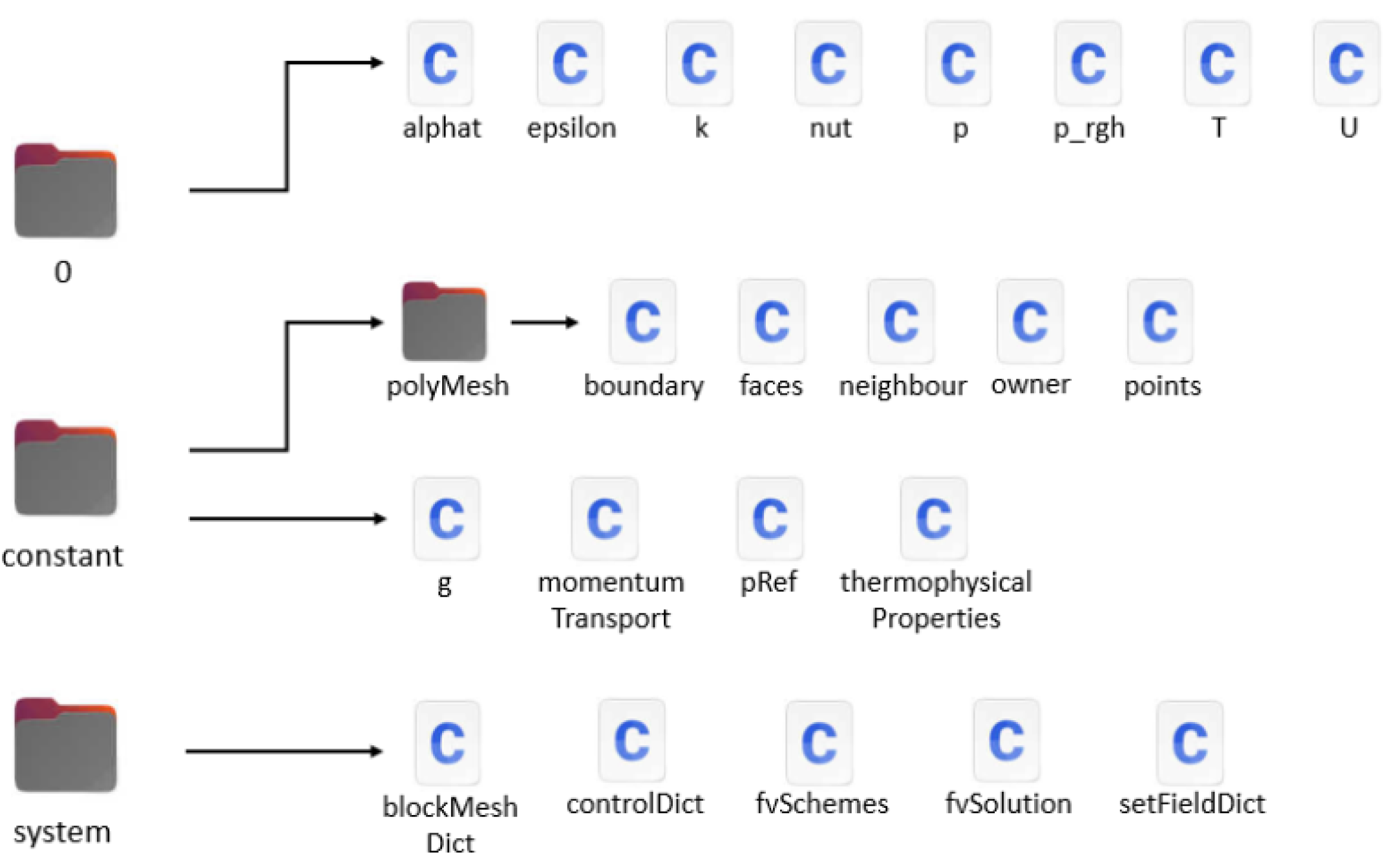
The constant directory stores values considered constant for the simulation, such as the gravitational acceleration (g). The turbulence model and its constants are included in momentumTransport. The fluid’s thermophysical properties are adjusted in the thermophysicalProperties file, enabling adaptation of the Prandtl Number and dynamic viscosity for the specific fluid.
Finally, in the “system” folder, the mesh configuration and simulation geometry are specified in the blockMeshDict file. Simulation time and data storage intervals are edited in controlDict. Although the algorithm in the OpenFOAM library has default data, it allows for adjusting values according to the required analysis and adding specific flow characteristics to be simulated.
The choice of interpolation functions is applied in the fvSchemes section. According to [20,21,22], the purpose of the interpolation function is to provide relationships between nodal points so that it is possible to calculate the value of the function and its derivatives at control volume interfaces. The aim is to propose a function with minimal error, involving the fewest nodal points necessary to generate a matrix. Figure A2 indicates the interpolation function used for each term of the simulation.
Figure A2.
File of interpolation functions.
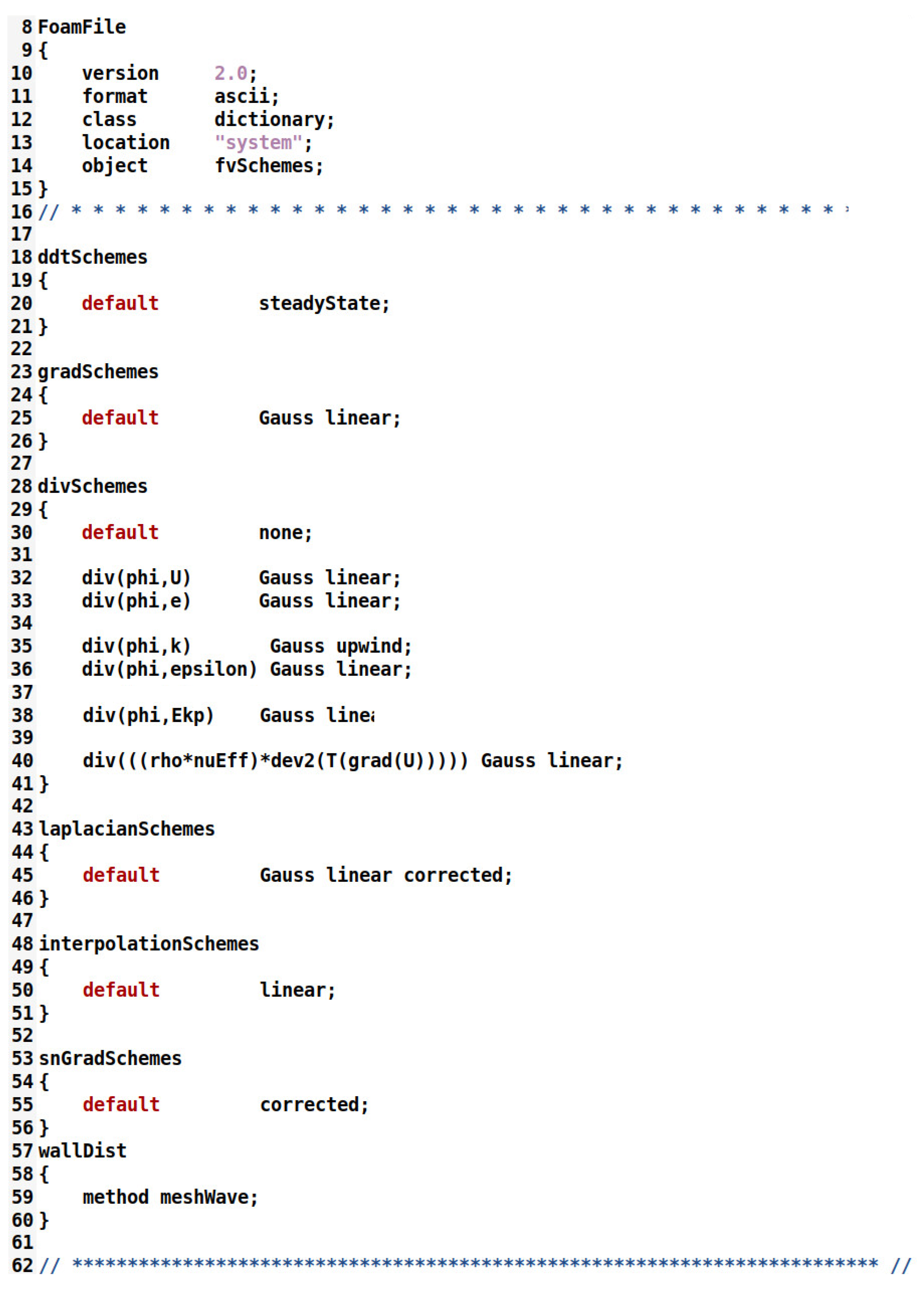
It is noted that two interpolation methods were used in the simulations: linear and upwind. This choice was based on studying the impact of interpolation functions on OpenFOAM results compared with the literature. Applying the upwind interpolation method to the divergence term for turbulent kinetic energy led to improved results.
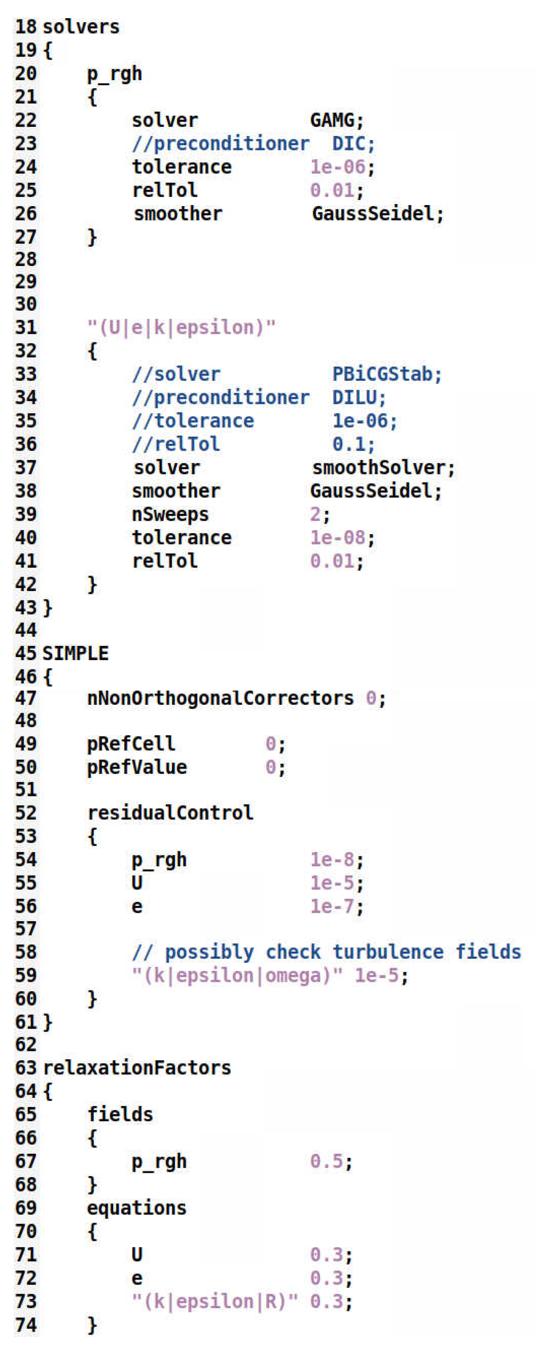
In the fvSolution file, convergence criteria, relaxation factors, and solver applications for the simulation are defined. Figure A3 presents the adopted values for all simulated cases.
Figure A3.
File for defining solvers, algorithms, tolerances, and relaxation factors.
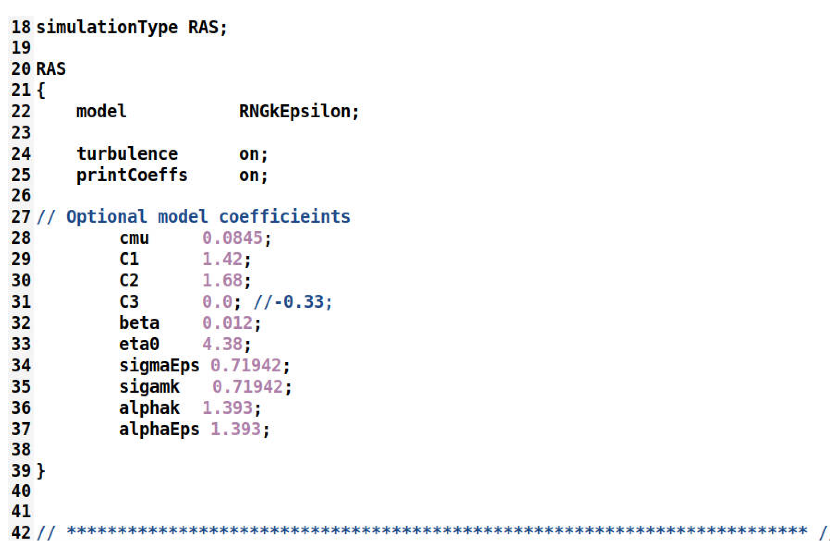
In OpenFOAM, the turbulence model is implemented in the momentumTransport file, where the model is selected, allowing for changes to constants from the default model if necessary (see Figure A4).
Figure A4.
File for turbulence model.
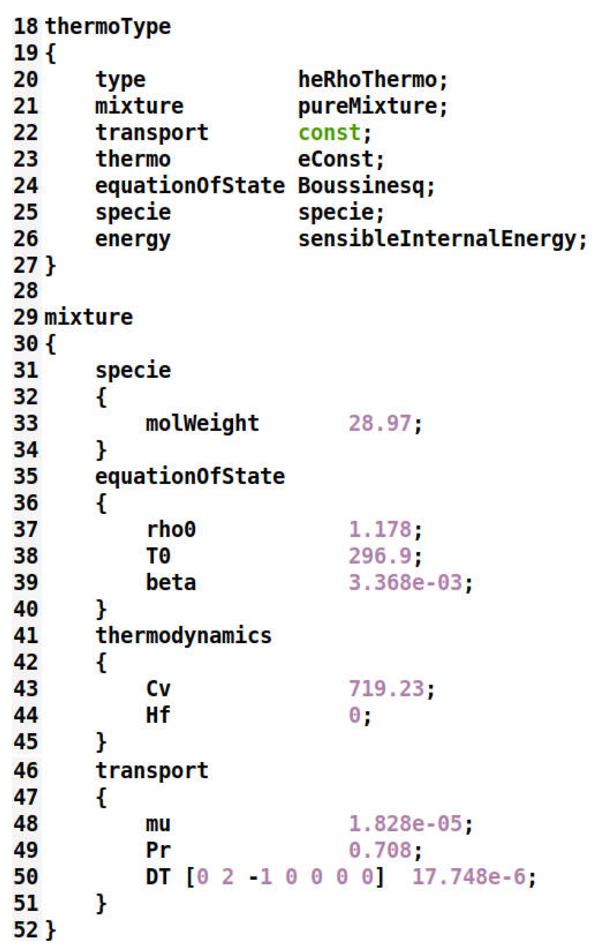
Thermophysical properties are adjusted in the thermophysicalProperties file. Thus, properties like Prandtl Number, dynamic viscosity, and the equation of state are set according to the working fluid, in this case, air. The Boussinesq approximation, applied as the equation of state in the energy balance equation (Equation (5)), requires values for , reference temperature, and reference density (see Figure A5). Values were assigned considering air as an ideal gas at 300 K.
Figure A5.
File for Thermophysical Properties.
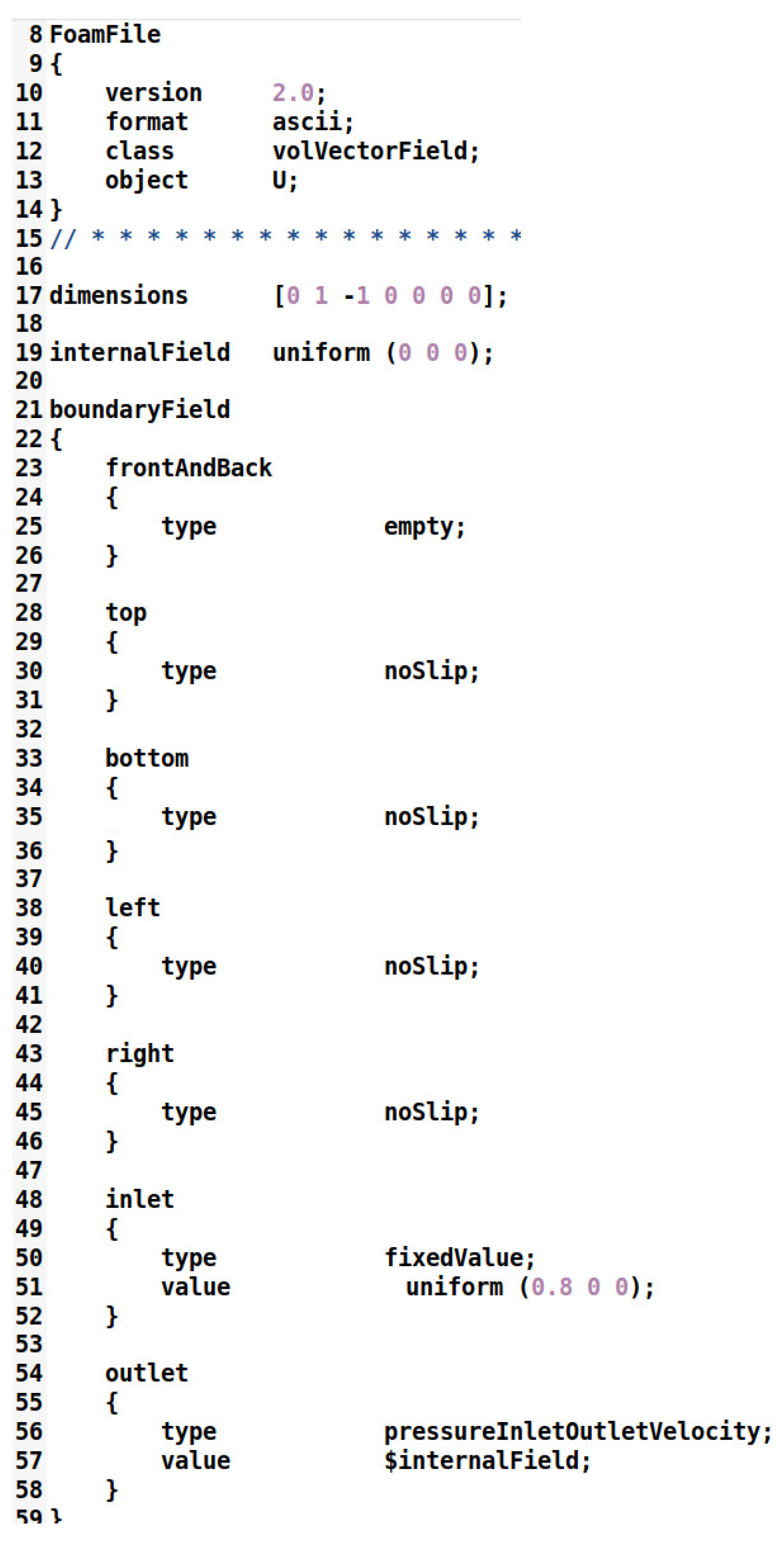
In the U file, velocity can be assigned for each boundary in the simulation geometry. Boundaries with no-slip conditions are labeled as noSlip. The boundary where air enters (inlet) has a fixed air velocity value. Figure A6 shows the velocity configuration file representing the flow simulated of the Table 1, following [13].
Figure A6.
File for velocity boundary conditions.
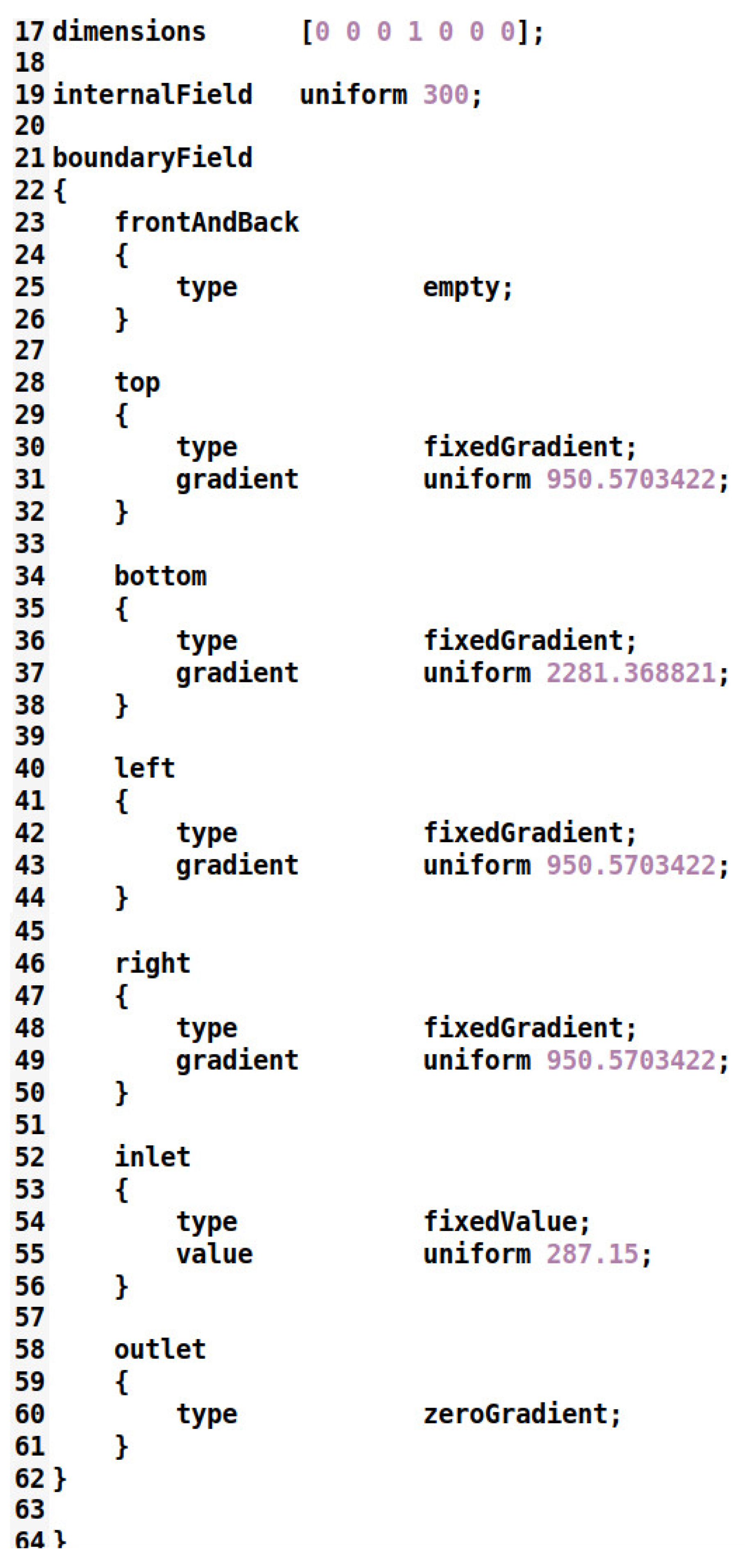
In OpenFOAM, the temperature gradient value is set in the T file for constant heat flux. Thus, the temperature gradient must be calculated based on the heat flux for each room surface except the inlet and outlet, see Equation (12). The inlet face sets the supply air temperature, while the outlet adopts a zero-gradient temperature boundary condition, which calculates temperature based on air thermal conductivity , as shown in Figure A7.
Figure A7.
File for energy boundary conditions.
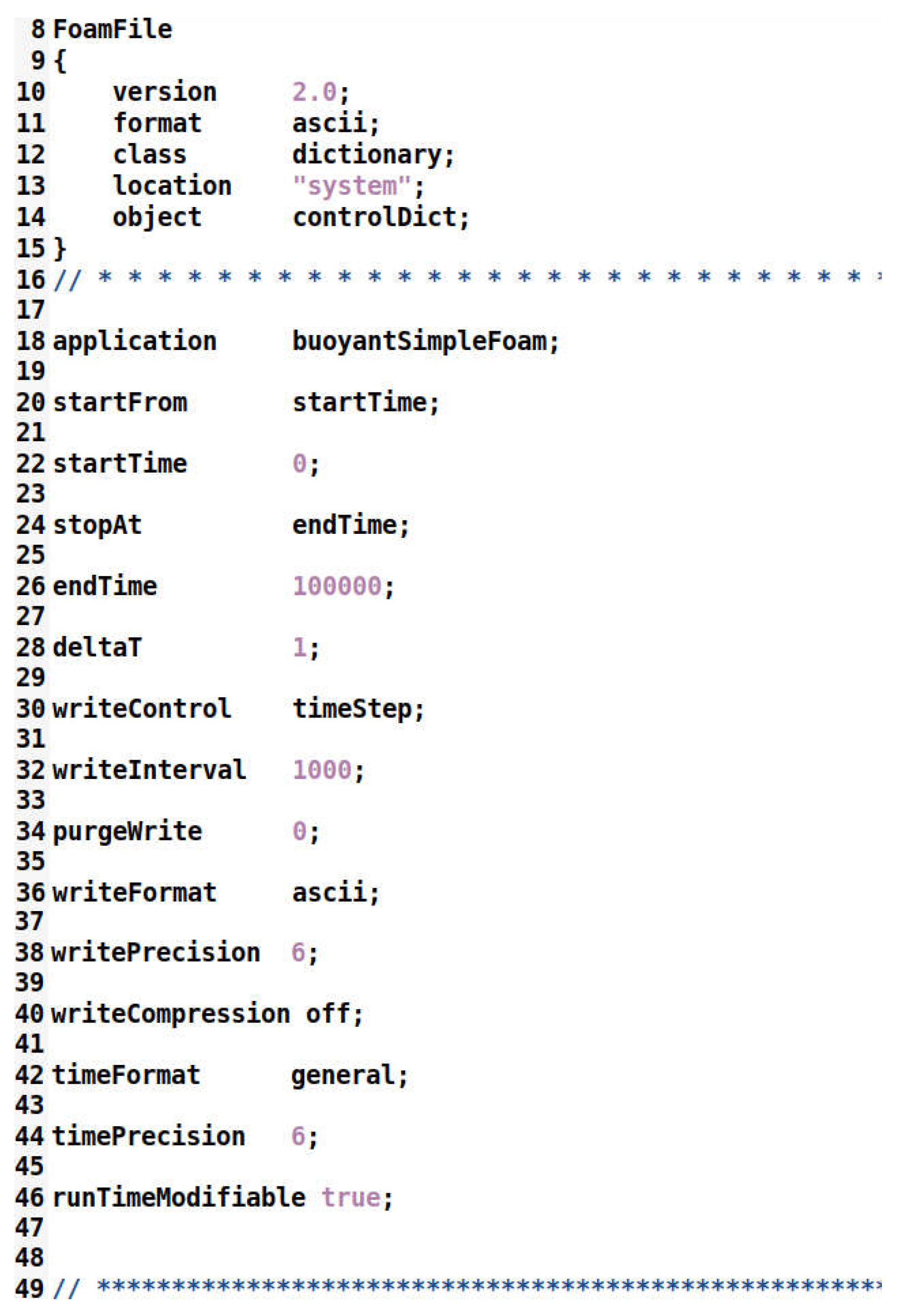
The solver used in the OpenFOAM simulation is modified in the controlDict file. In this command, the buoyantSimpleFoam solver is specified. The number of iterations and data logging intervals are also modified in this file, as shown in Figure A8.
The checkMesh command verifies any errors in the generated mesh. The numerical solution is obtained by implementing the buoyantSimpleFoam command, which performs calculations to achieve convergence.
Visual analysis of results is conducted in ParaView software using the paraFoam command in the Linux terminal. These programs were chosen as they are open-source, as is OpenFOAM. This approach allows visualization and extraction of simulation data. Data can also be exported to spreadsheets to create velocity, temperature, or pressure graphs related to the flow.
Figure A8.
ControlDict File.
References
- Mehrdad, R.; Habtamu Bayera, M.; Natasa, N. Building Retrofitting through Coupling of Building Energy Simulation-Optimization Tool with CFD and Daylight Programs. Energies 2021, 2180, 1–23. [Google Scholar]
- Matthew, B.; Daniel, M.; Simon Paul, B. Humidity Distribution in High-Occupancy Indoor Micro-Climates. Energies 2021, 681, 1–16. [Google Scholar]
- Stoecker, W.F.; Jones, J.W. Refrigeração e ar condicionado; McGraw-Hill do Brasil, 1985.
- Daehyun, K.; Hyunmuk, L.; Jongmin, M.; Jinsoo, P.; Gwanghoon, R. Heating Performances of a Large-Scale Factory Evaluated through Thermal Comfort and Building Energy Consumption. Energies 2021, 5617, 1–15. [Google Scholar]
- Cheng, Y.; Lin, Z. Experimental study of airflow characteristics of stratum ventilation in a multi–occupant room with comparison to mixing ventilation and displacement ventilation. Indoor Air 2015, 25, 662–671. [Google Scholar] [CrossRef] [PubMed]
- Che, W.W.; Tso, C.Y.; Sun, L.; Ip, D.Y.; Lee, H.; Chao, C.Y.; Lau, A.K. Energy consumption, indoor thermal comfort and air quality in a commercial office with retrofitted heat, ventilation and air conditioning (HVAC) system. Energy and Buildings 2019, 201, 202–215. [Google Scholar] [CrossRef]
- ASHRAE. ASHRAE STANDARD 55. Thermal Environmental Conditions for Human Occupancy, 2013.
- Limane, A.; Fellouah, H.; Galanis, N. Three-dimensional OpenFOAM simulation to evaluate the thermal comfort of occupants, indoor air quality and heat losses inside an indoor swimming pool. Energy and Buildings 2018, 167, 49–68. [Google Scholar] [CrossRef]
- SIMSCALE. Tutorial: Thermal Comfort Parameters for HVAC Simulations, 2016.
- Liu, S.; Clark, J.; Novoselac, A. Air diffusion performance index (ADPI) of overhead-air-distribution at low cooling loads. Energy and Buildings 2017, 134, 271–284. [Google Scholar] [CrossRef]
- Samiuddin, S.; Budaiwi, I.M. Assessment of thermal comfort in high-occupancy spaces with relevance to air distribution schemes: A case study of mosques. Building Services Engineering Research and Technology 2018, 39, 572–589. [Google Scholar] [CrossRef]
- Ng, K.; Kadirgama, K.; Ng, E. Response surface models for CFD predictions of air diffusion performance index in a displacement ventilated office. Energy and Buildings 2008, 40, 774–781. [Google Scholar] [CrossRef]
- Youssef, A.A.; Mina, E.M.; ElBaz, A.R.; AbdelMessih, R.N. Studying comfort in a room with cold air system using computational fluid dynamics. Ain Shams Engineering Journal 2018, 9, 1753–1762. [Google Scholar] [CrossRef]
- Córdova-Suárez, M.; Tene-Salazar, O. .; Tigre-Ortega, F..; Carrillo-Ríos, S..; Córdova-Suárez, D..; TapiaVasco, L..; Quesada-Revelo, D. An OpenFOAM simulation of the natural ventilation system in a university chemical laboratory. E3S Web Conf. 2020, 167, 04003. [Google Scholar] [CrossRef]
- ASHRAE. ASHRAE STANDARD 55. Thermal Environmental Conditions for Human Occupancy, 2013.
- Launder, B.; Spalding, D. The numerical computation of turbulent flows. Computer Methods in Applied Mechanics and Engineering 1974, 3, 269–289. [Google Scholar] [CrossRef]
- Maria, H.; Piotr, C.; Zbigniew, P. Eddy–Viscosity Reynolds-Averaged Navier–Stokes Modeling of Air Distribution in a Sidewall Jet Supplied into a Room. Energies 2024, 1261, 1–19. [Google Scholar]
- da Silveira Neto, A. Escoamentos Turbulentos Análise Física e Modelagem Teórica; Composer Arte e Editora, 2020.
- OpenFOAM. About OpenFOAM, 2021.
- Versteeg, H.; Malalasekera, W. An Introduction to Computational Fluid Dynamics: The Finite Volume Method; Pearson Education, 2007.
- Patankar, S. Numerical Heat Transfer and Fluid Flow; CRC Press, 2018. [CrossRef]
- Maliska, C.R. Transferência de Calor e Mecânica dos Fluidos Computacional; LTC, 1995.
Figure 1.
The two-dimensional room model used in the numerical study generated by the OpenFOAM blockMesh algorithm: room geometry.
Figure 1.
The two-dimensional room model used in the numerical study generated by the OpenFOAM blockMesh algorithm: room geometry.
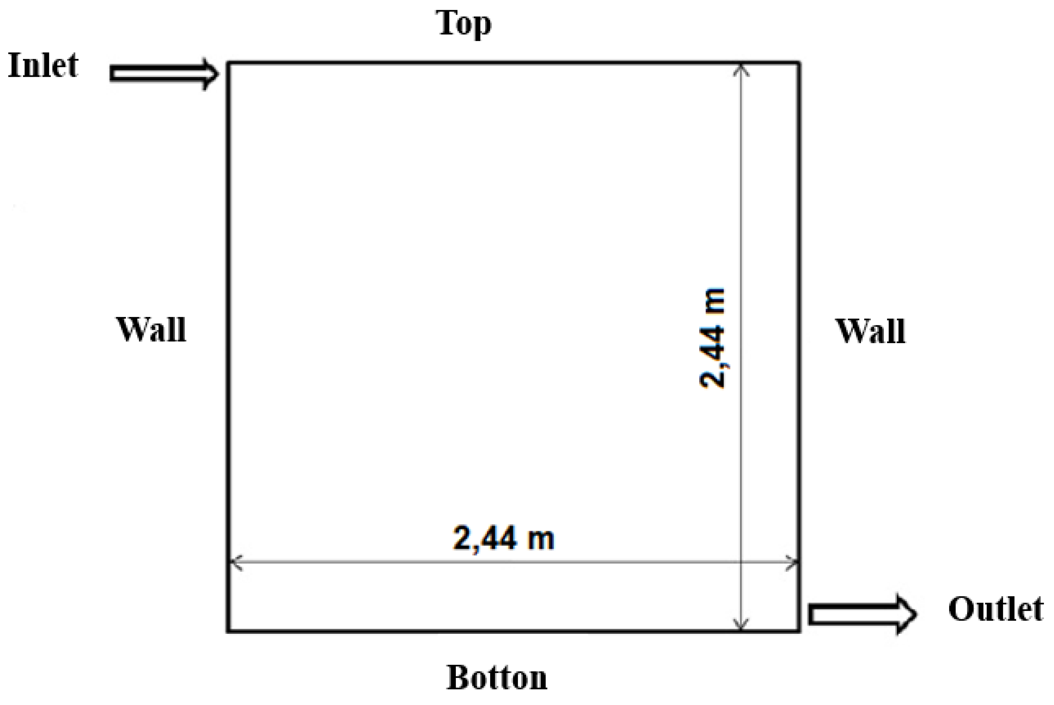
Figure 2.
The two-dimensional room model used in the numerical study generated by the OpenFOAM blockMesh algorithm: mesh with 44 x 44 non-uniform volumes.
Figure 2.
The two-dimensional room model used in the numerical study generated by the OpenFOAM blockMesh algorithm: mesh with 44 x 44 non-uniform volumes.
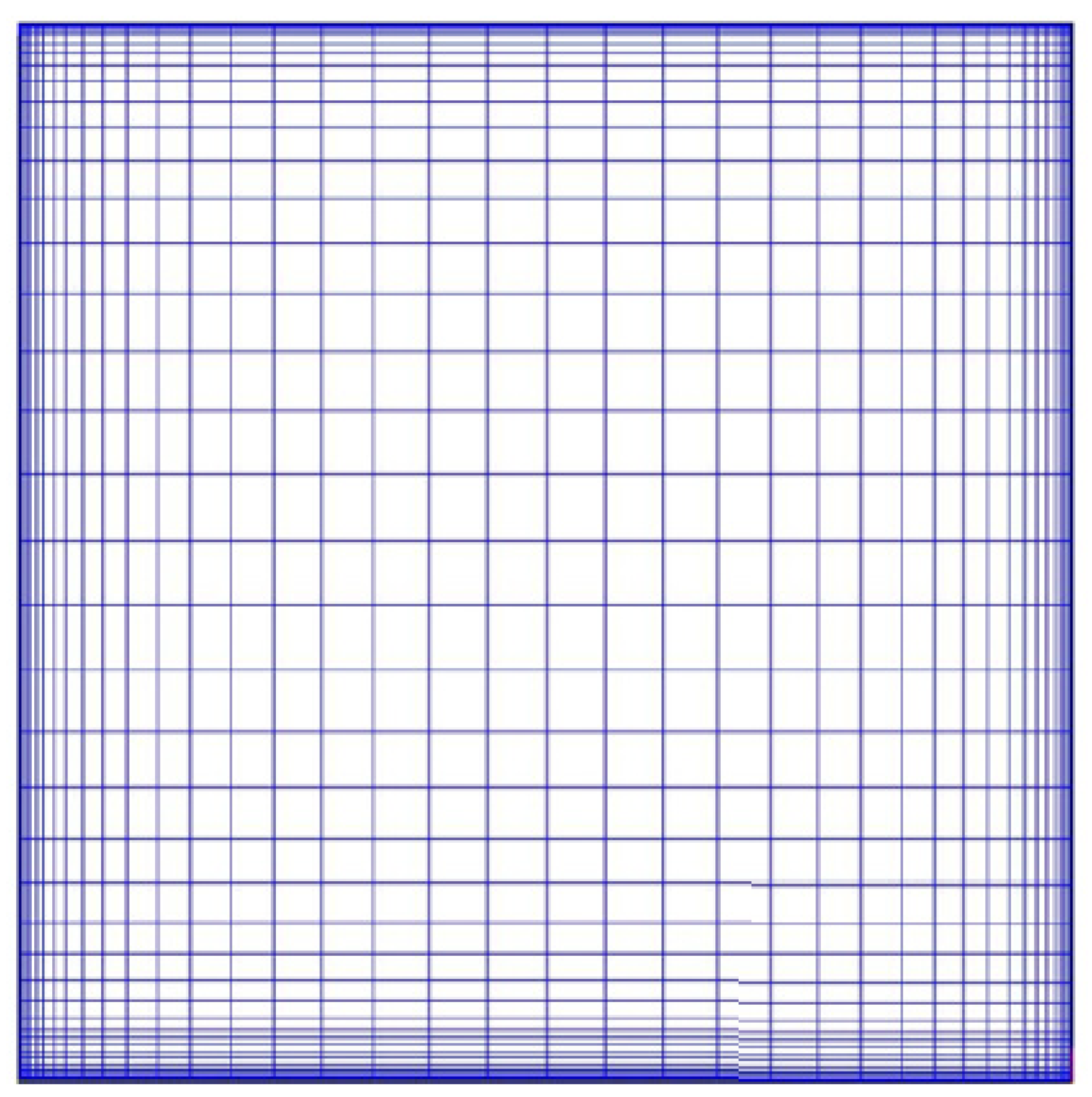
Figure 3.
Vertical profile of horizontal velocity, obtained at x/L=0.5: Mesh refinement.
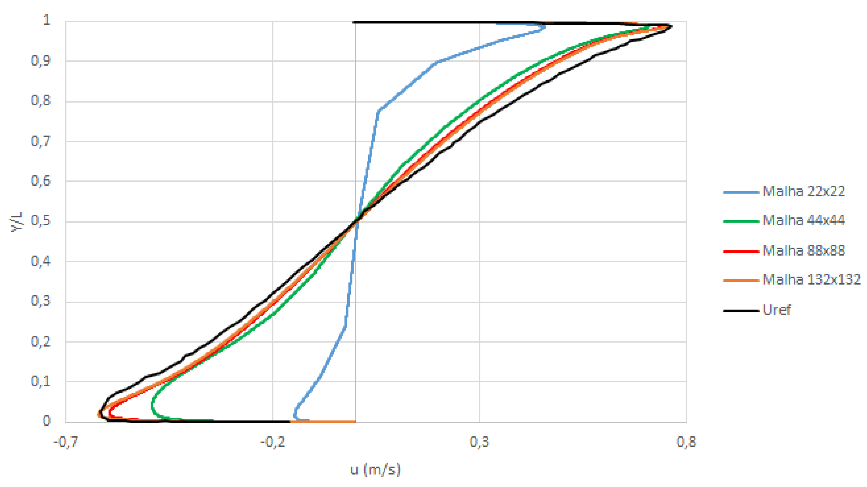
Figure 4.
Vertical profile of horizontal velocity, obtained at x/L=0.5: Interpolation function.
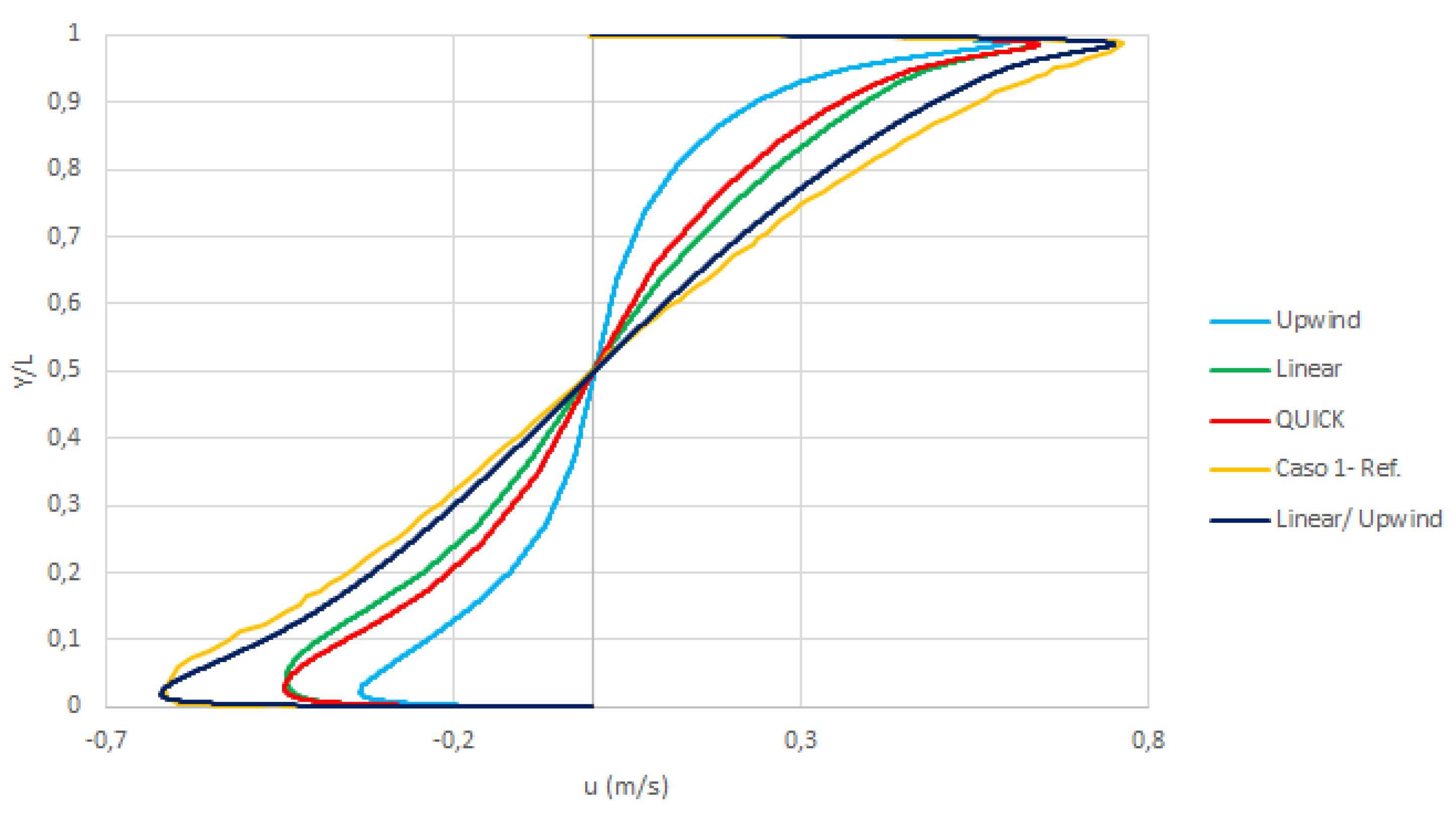
Figure 5.
Air inlet and outlet positions.
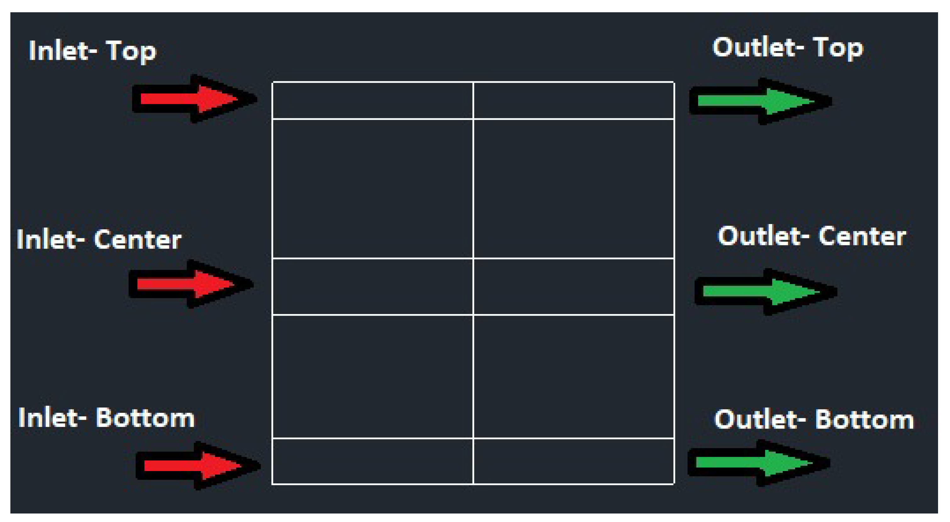
Figure 6.
Temperature field: air supply both inlet and outlet at the bottom.
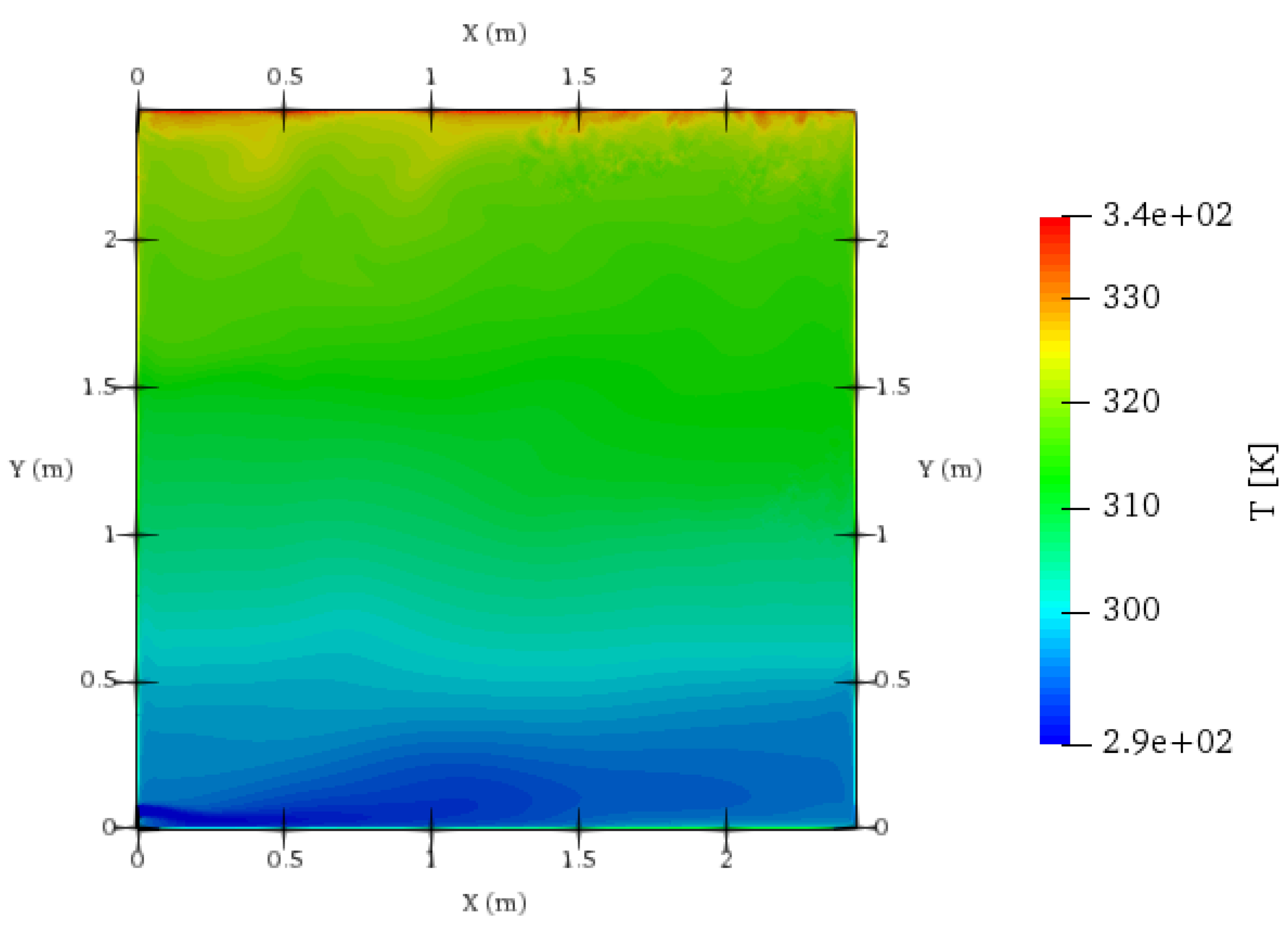
Figure 7.
Temperature field: air supply both inlet and outlet at the center.
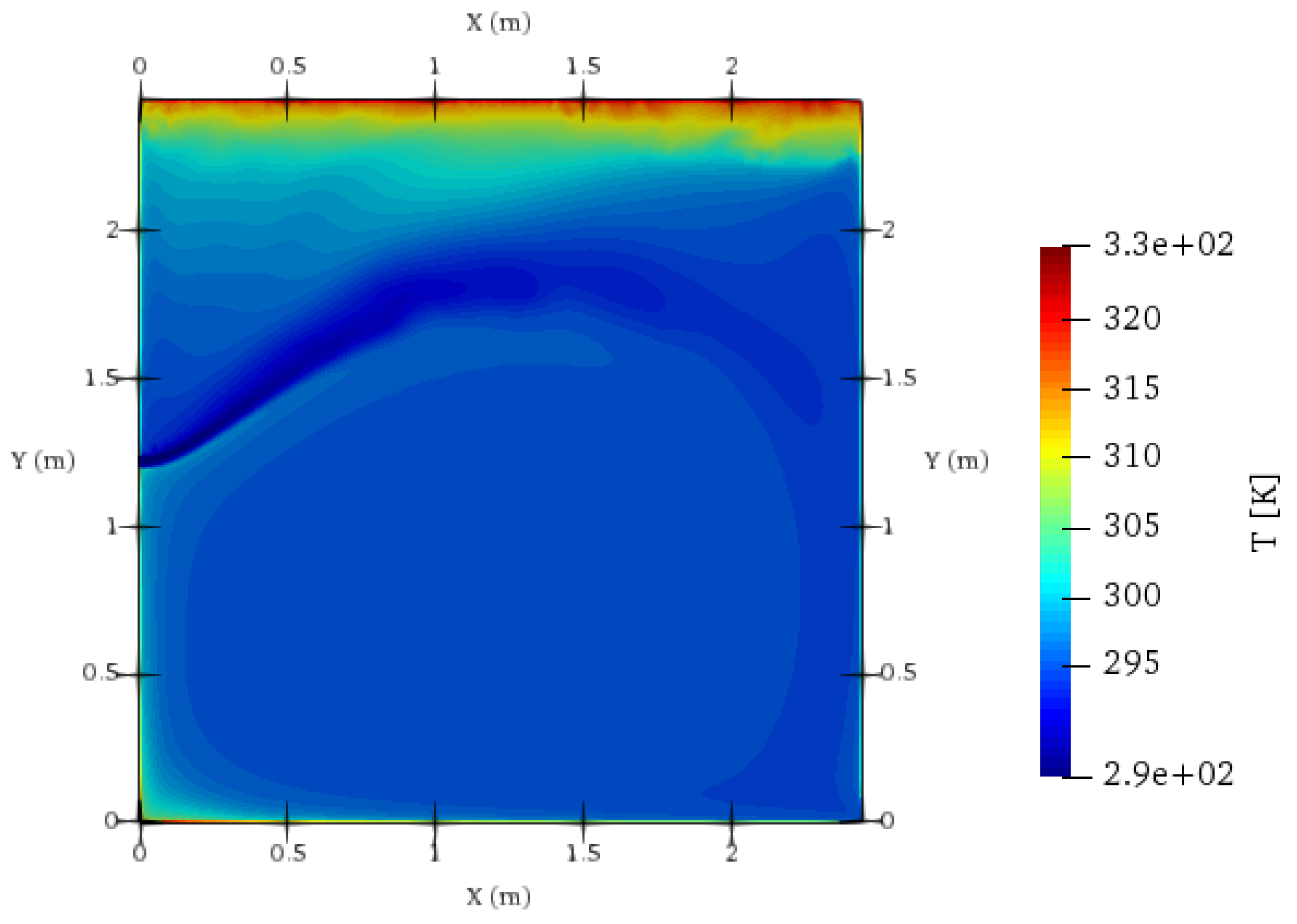
Figure 8.
Simulations with air supply and exhaust at the top: Temperature field.
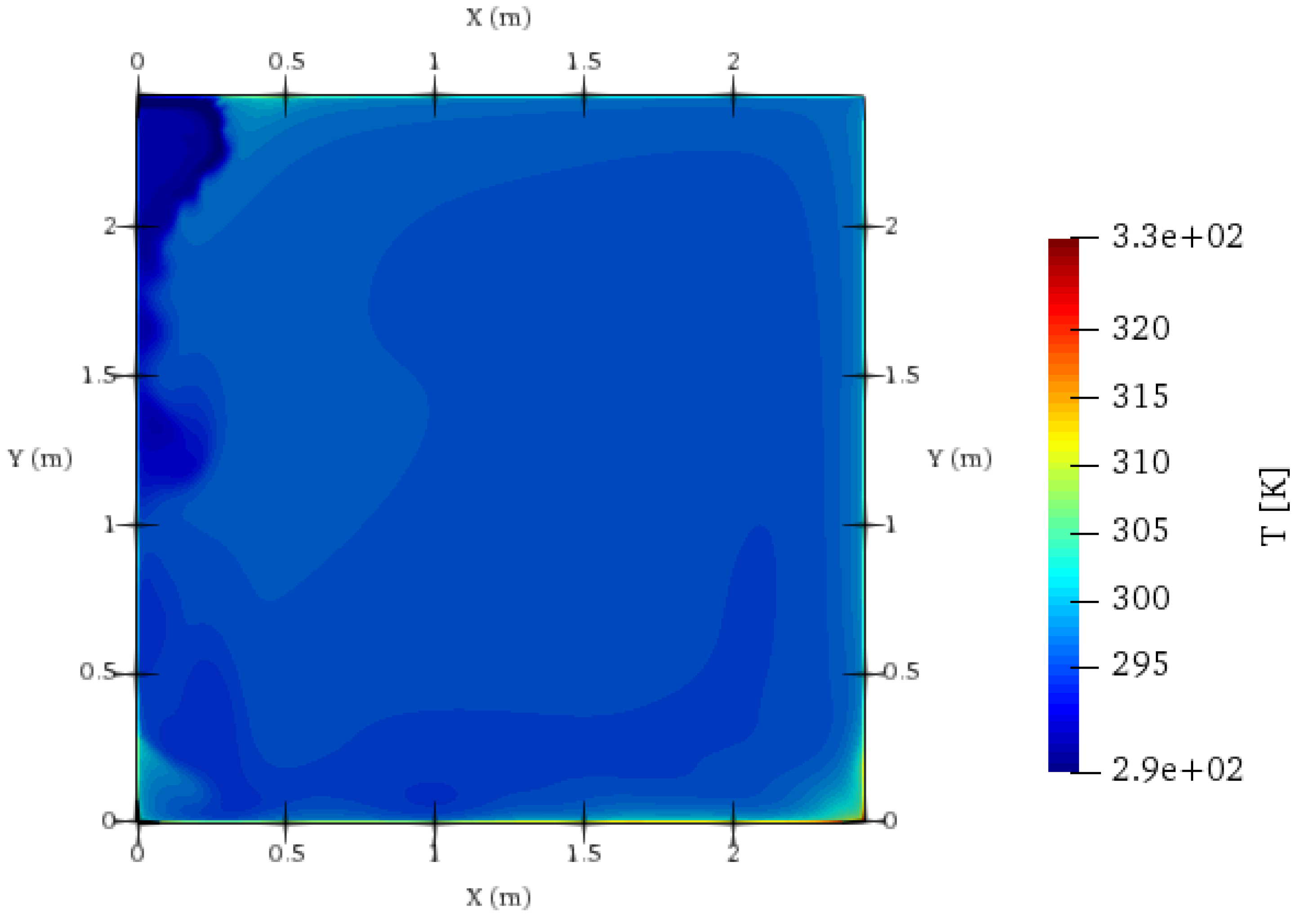
Figure 9.
Simulations with air supply and exhaust at the top: Streamlines.
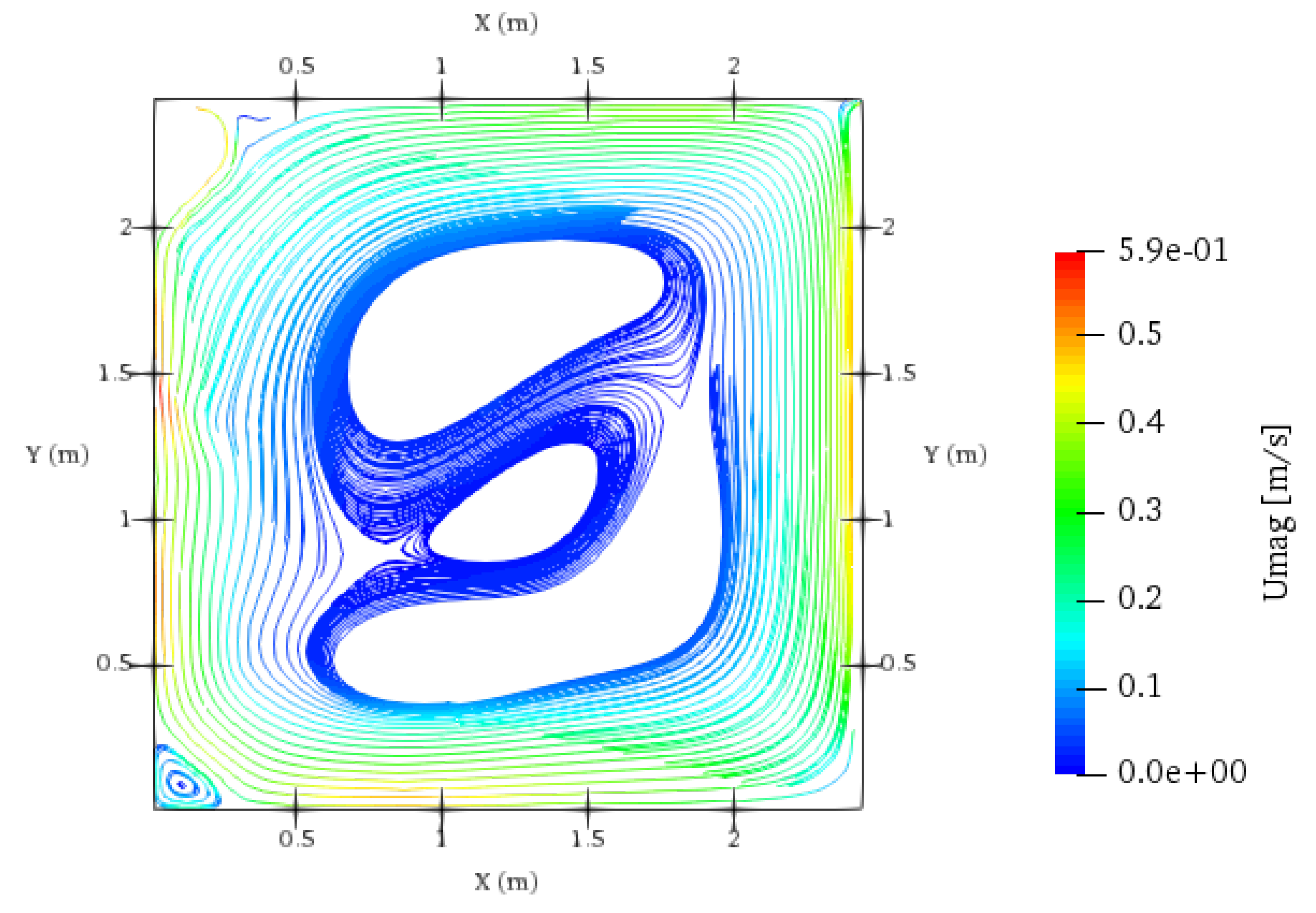

Table 1.
Boundary and initial conditions adopted.
| Condition | U | T | |||||
| initial | (0.0,0.0,0.0) | 0.0 | 300 | 0.10 | 0.01 | 0.0 | 0.0 |
| inlet | (0.8,0.0,0.0) | 287.15 | 0.0 | 4.0e-6 | 0.0 | 0.0 | |
| outlet | 0.0 | 0.0 | 4.0e-6 | 0.0 | 0.0 | ||
| left, right, top | (0.0,0.0,0.0) | 0.0 | 4.0e-6 | 0.0 | 0.0 | ||
| botton | (0.0,0.0,0.0) | 0.0 | 4.0e-6 | 0.0 | 0.0 | ||
| front, back | empty | empty | empty | empty | empty | empty | empty |
Table 2.
Parameters for the factorial design.
| Inlet position | Outlet position | Air supply velocity (m/s) |
|---|---|---|
| Bottom | Bottom | 0.5 |
| Center | Center | 0.8 |
| Top | Top | 1.2 |
Disclaimer/Publisher’s Note: The statements, opinions and data contained in all publications are solely those of the individual author(s) and contributor(s) and not of MDPI and/or the editor(s). MDPI and/or the editor(s) disclaim responsibility for any injury to people or property resulting from any ideas, methods, instructions or products referred to in the content. |
© 2024 by the authors. Licensee MDPI, Basel, Switzerland. This article is an open access article distributed under the terms and conditions of the Creative Commons Attribution (CC BY) license (http://creativecommons.org/licenses/by/4.0/).
Copyright: This open access article is published under a Creative Commons CC BY 4.0 license, which permit the free download, distribution, and reuse, provided that the author and preprint are cited in any reuse.


