Submitted:
29 October 2024
Posted:
30 October 2024
You are already at the latest version
Abstract
Keywords:
1. Introduction
2. Related Work
2.1. Zero-Shot Generalization
2.2. Artificial Potential Field
2.3. Hierarchical Reinforcement Learning
- 1)
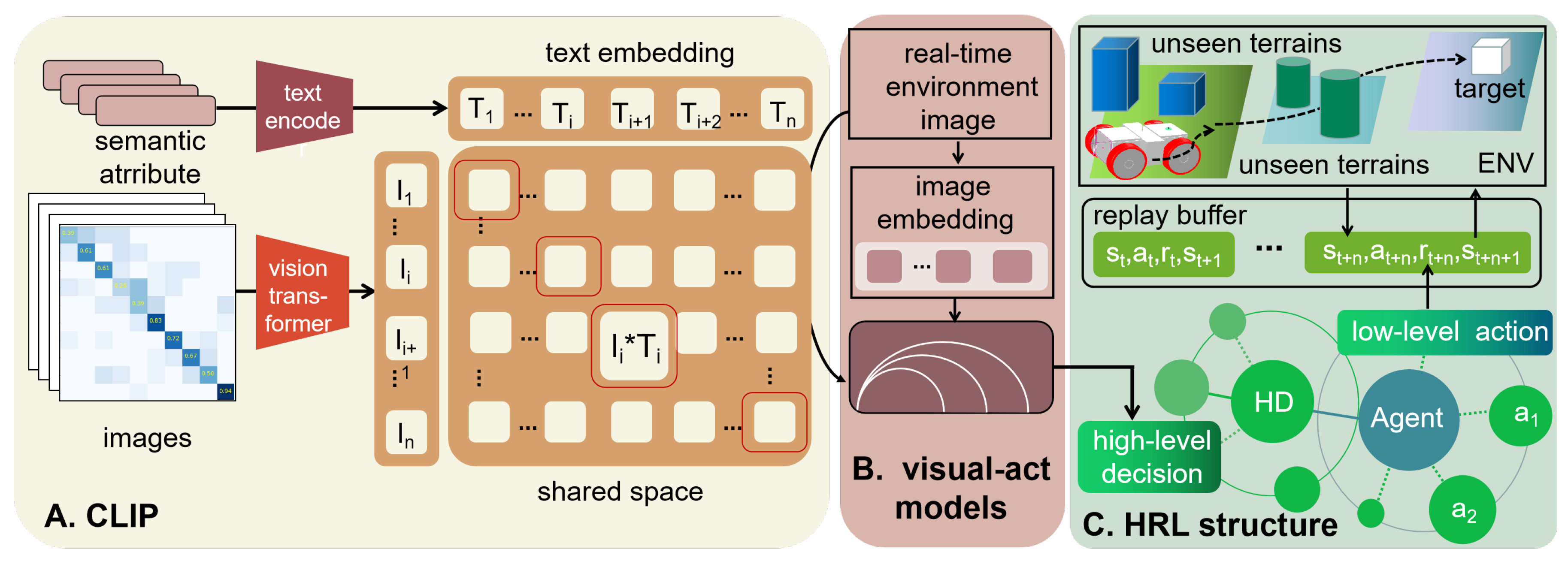
- The proposed method first fuses ZSL into the reinforcement learning process for robot path planning. After integrating the unseen semantic information, the agent becomes more intelligent regarding path selection and training cost control.
- 2)
- A reasonable fusion architecture is proposed specifically. ZSL is utilized on a high level to infer correct macro-actions for previously unseen objects or situations based on learned semantic relationships. Then, the HRL follows cues offered by zero-shot learning to make decisions effectively in specific path selections.
- 3)
- Detailed performance analysis is provided for the proposed combined learning framework. The simulation results corroborate the proposed method’s capability of leveraging visual cues for decisions and modifying agents’ actions.
3. Proposed Method
3.1. Contrastive Language-Image Pre-Trained Model
3.2. Visual-Act Model
Algorithm 1: Optimized model for high-level macro-action decision making in action selection |
|
Algorithm 2: Hierarchical path planning |
|
3.3. Hierarchical Policy
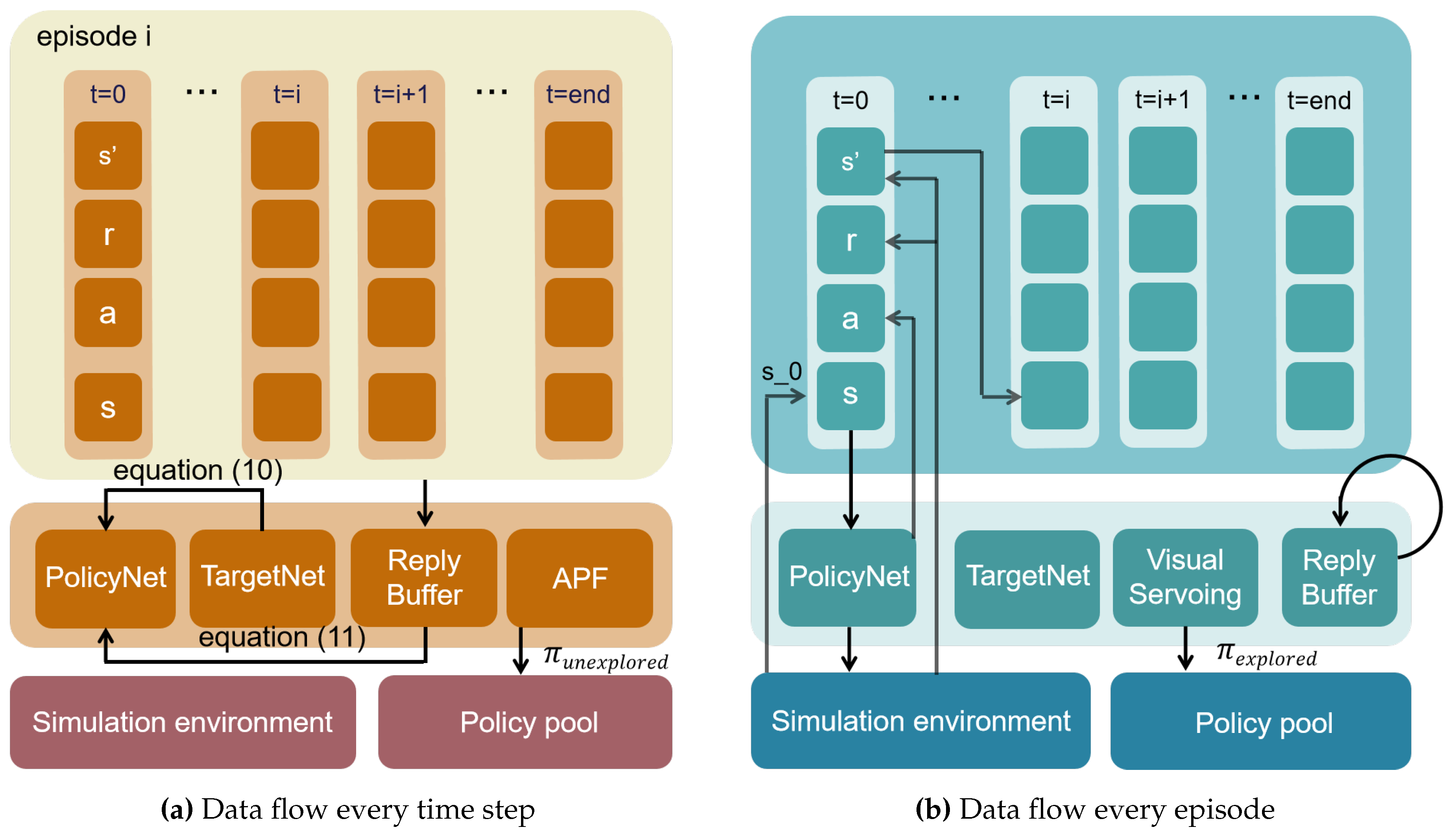
4. Simulation
- 1)
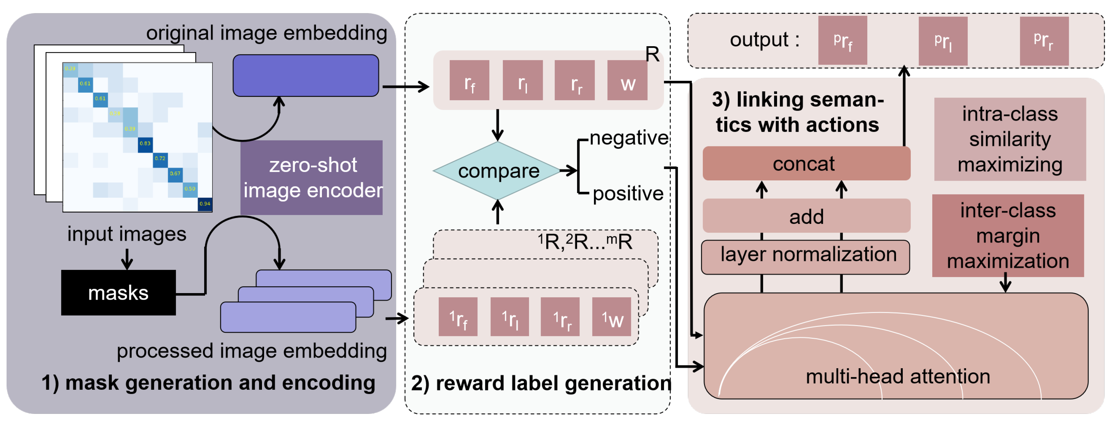
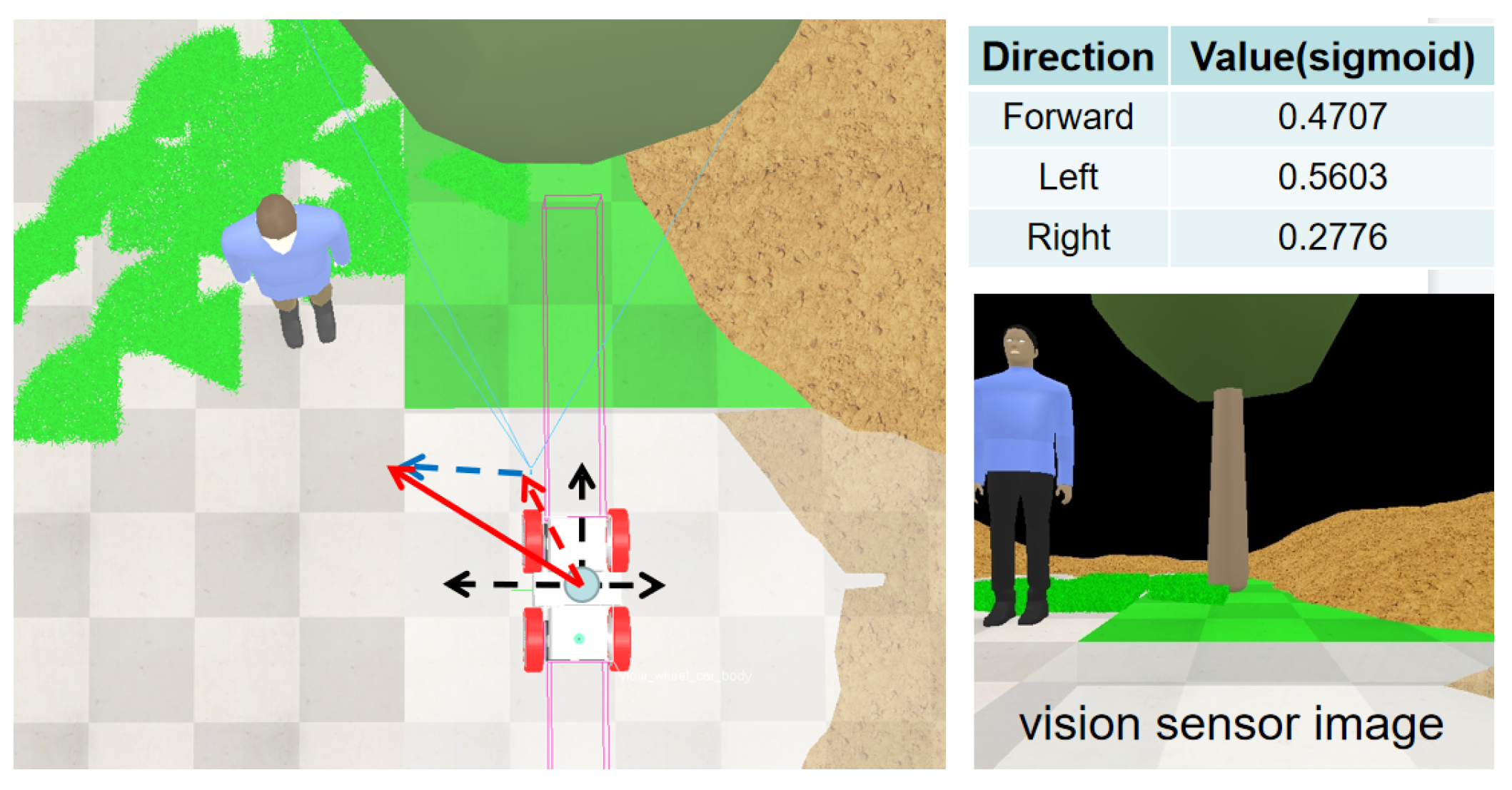
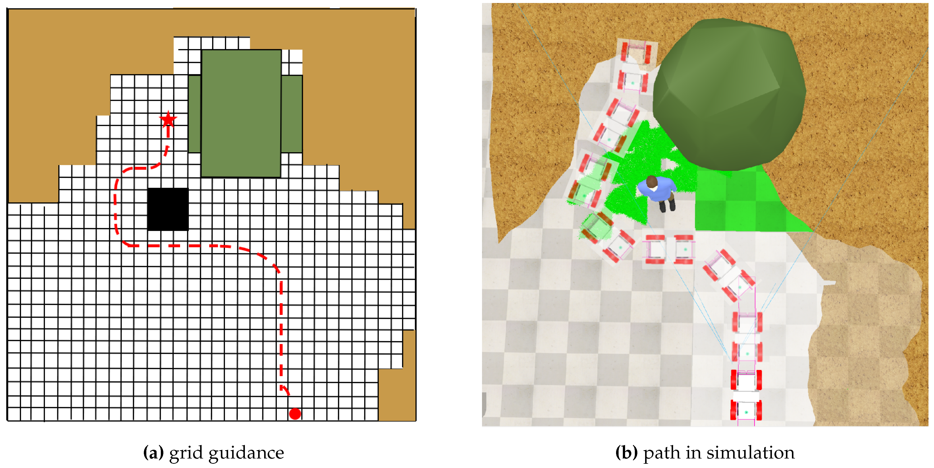
- The leveraging visual cues for actions selection model does focus on certain objects in images to form correspondent advice for action selection.
- 2)
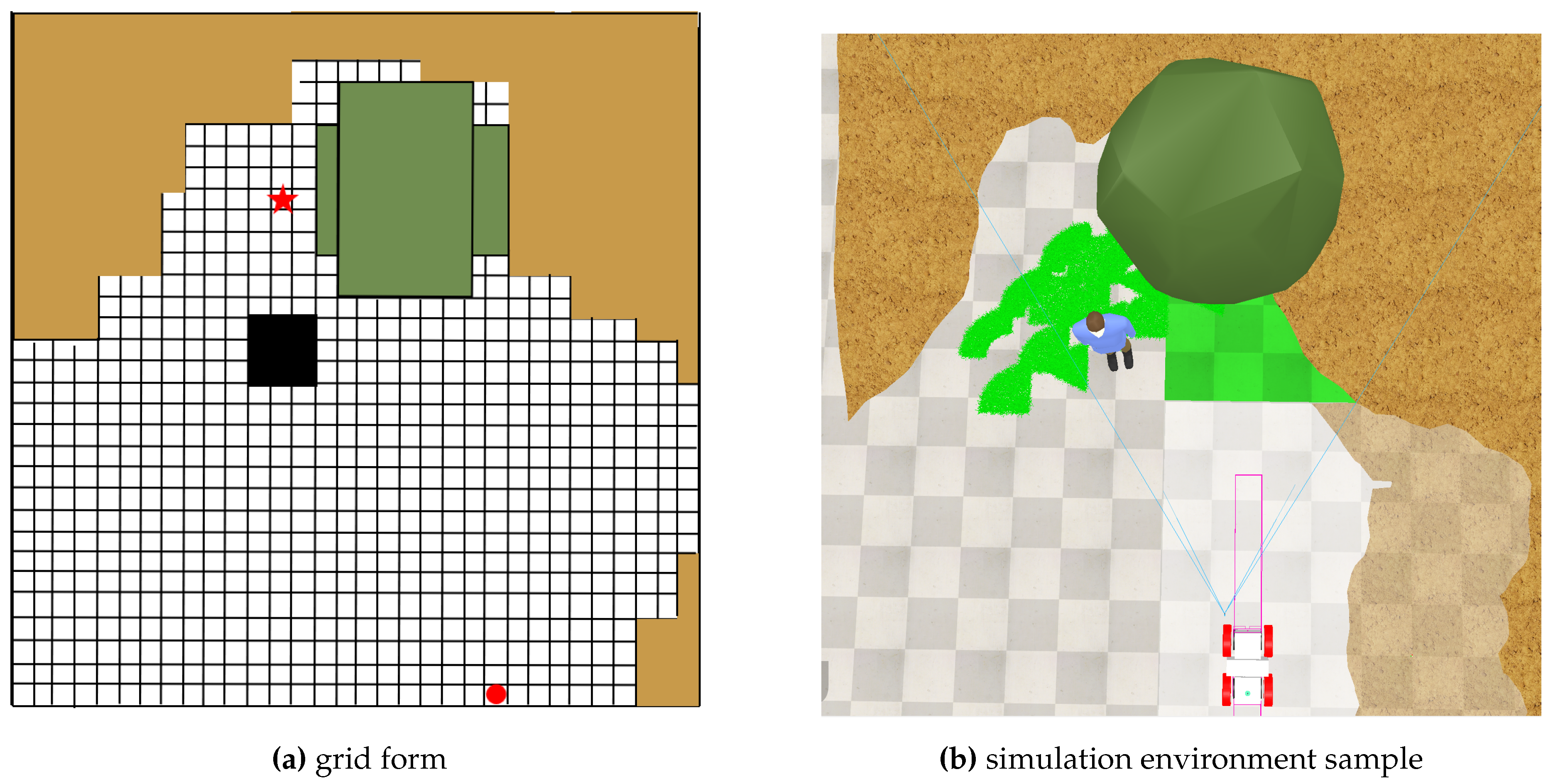
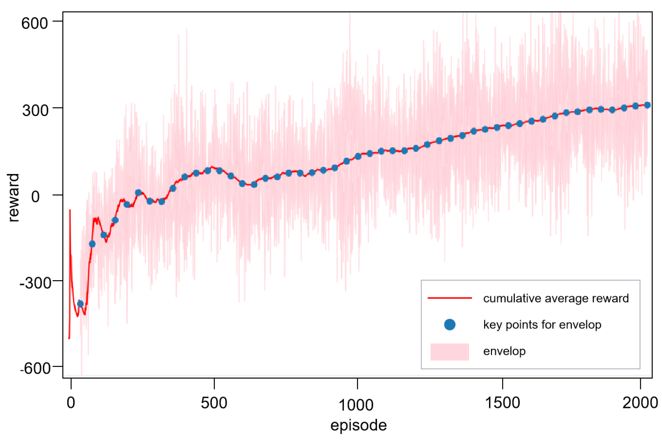
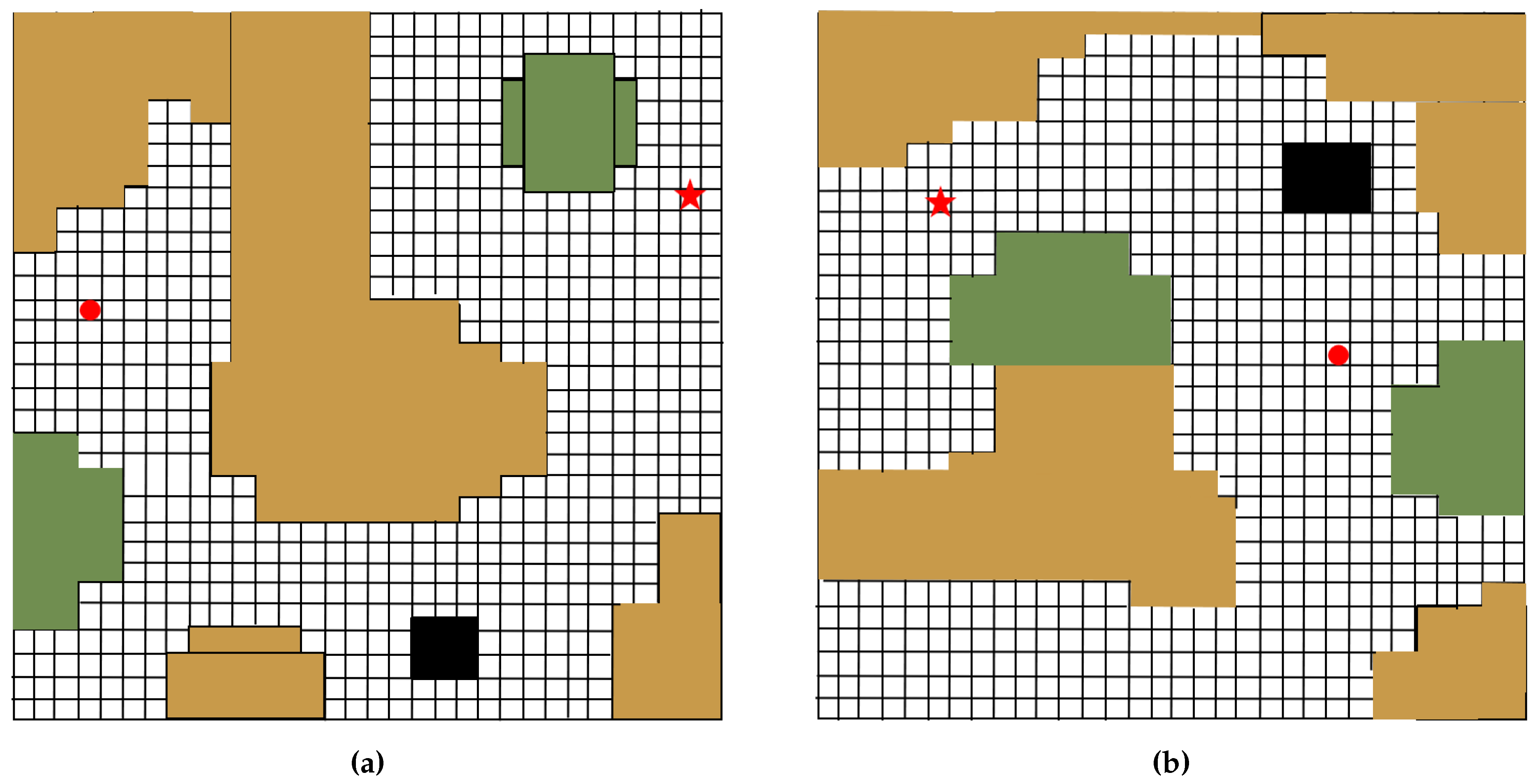
- To assess the modal’s capability to generate across environments, we conduct path planning simulation in unseen environments, which proves that the proposed method can reduce training time and increase exploring efficiency.
- 3)
- The proposed method performs well when combined with reinforcement learning.
4.1. Simulation Setting
4.2. Simulation Process
4.3. Assessment of the Visual-Act Model
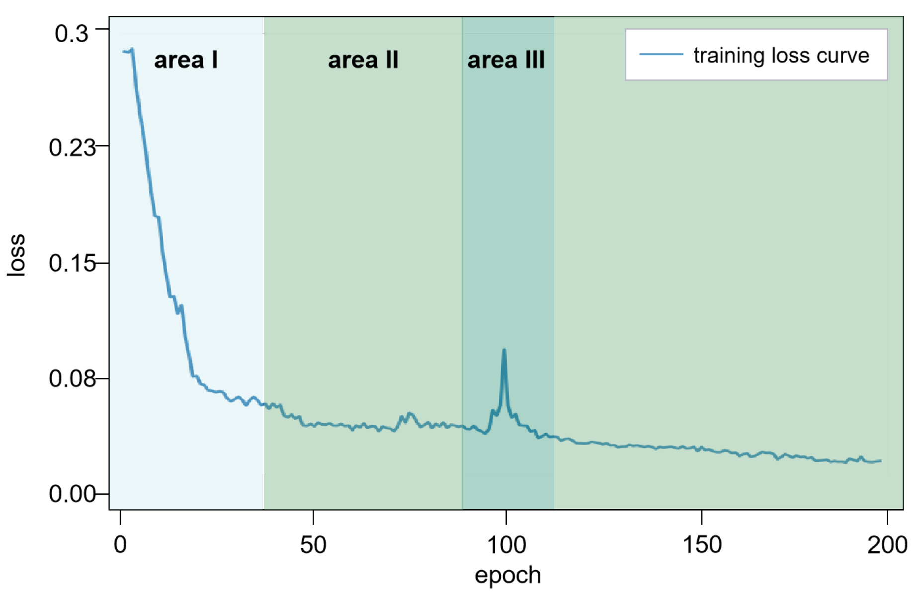
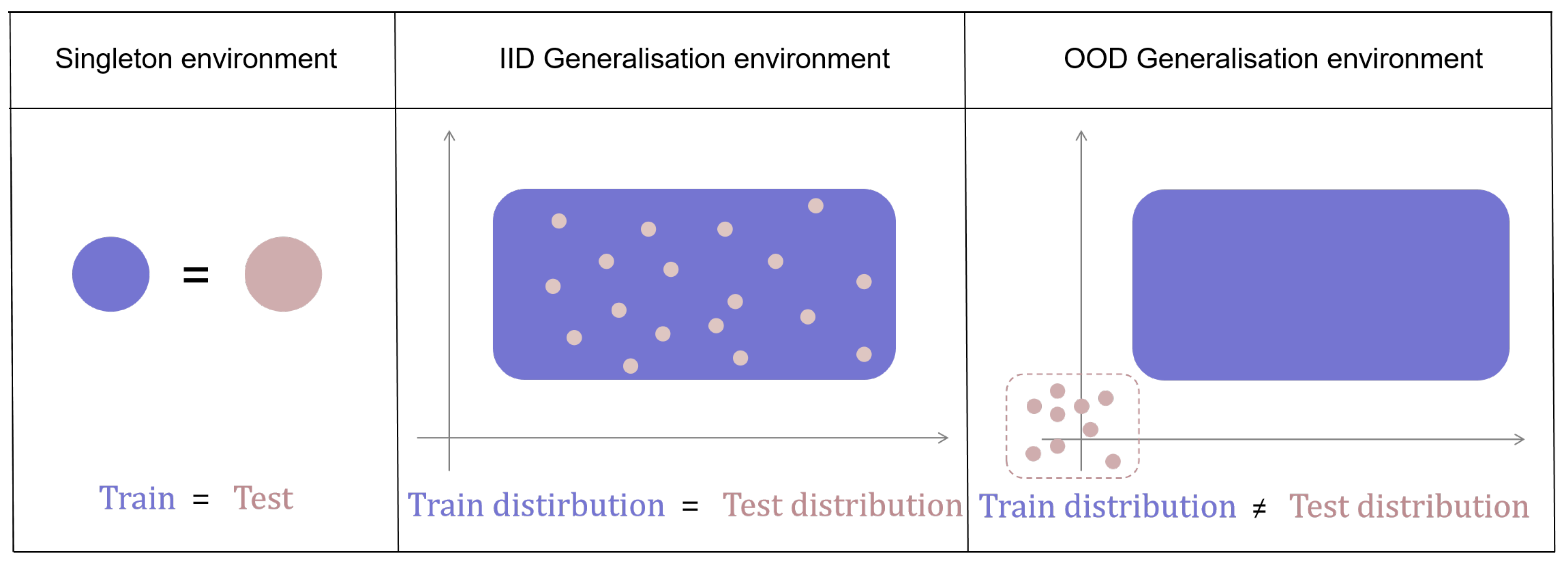
4.4. Performance Assessment under Singleton Environment
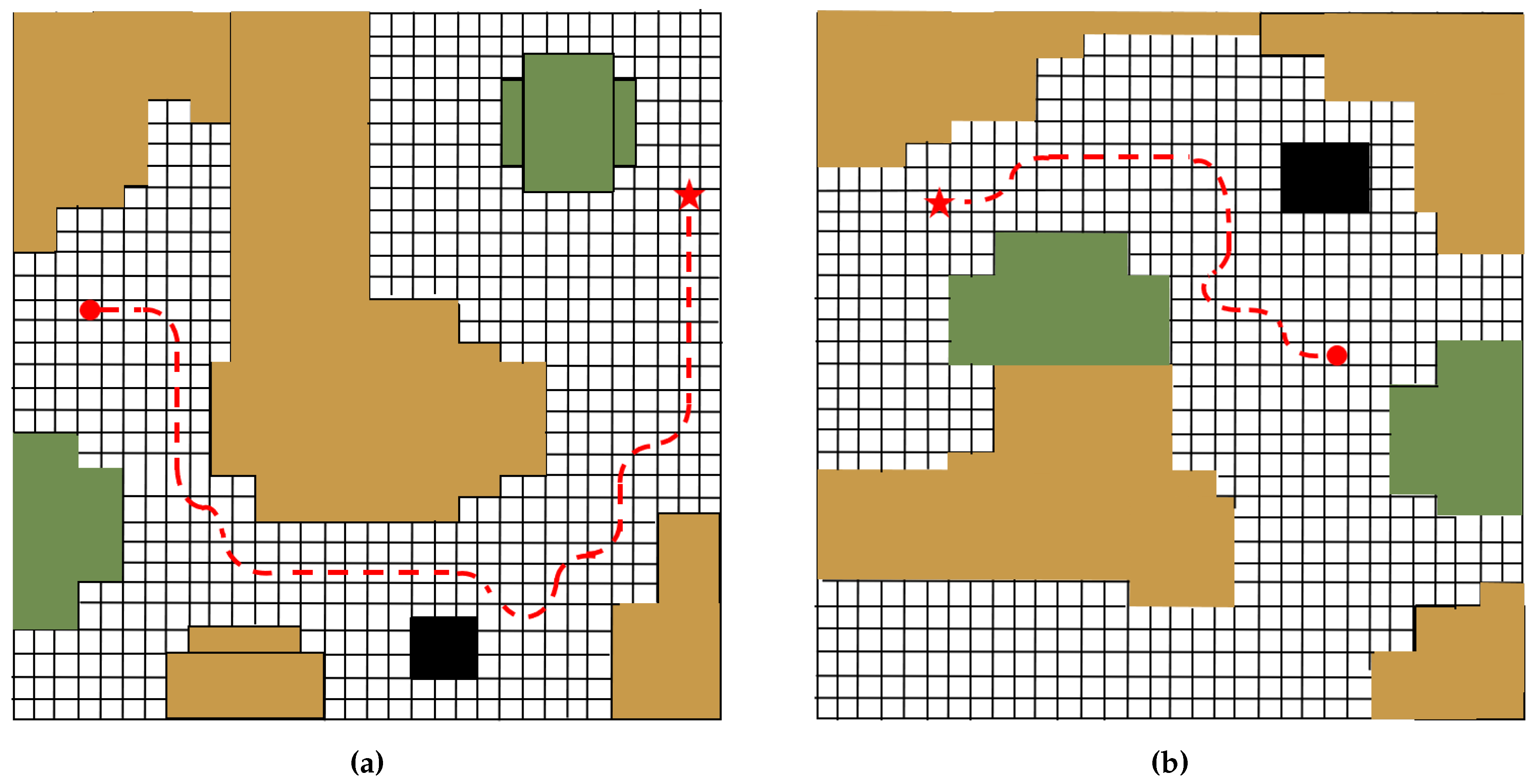
4.5. Performance Assessment under Test Environments
| Environment | S1 | C2 | 3 | 4 |
|---|---|---|---|---|
| (a) | 9.25% | 8.53% | 21.62% | 2.64% |
| (b) | 3.31% | 14.72% | 11.91% | 3.12% |
| (c) | 16.28% | 7.34% | 31.88% | 0.65% |
5. Conclusion
References
- Duchoň, F. Path planning with modified a star algorithm for a mobile robot. Procedia engineering 2014, 96, 59–69. [Google Scholar] [CrossRef]
- Luo, M.; Hou, X.; Yang, J. Surface optimal path planning using an extended Dijkstra algorithm. IEEE Access 2020, 8, 147827–147838. [Google Scholar] [CrossRef]
- Kennedy, J.; Eberhart, R. Particle swarm optimization. Proceedings of international conference on neural networks, Perth, Australia, Nov 27-Dec 1 1995; pp. 1942–1948. [Google Scholar]
- Shi, Y.; Eberhart, R. A modified particle swarm optimizer. Proceedings of IEEE international conference on evolutionary computation, Anchorage, USA, 4-9 May 1998; pp. 69–73. [Google Scholar]
- Grisetti, G.; Kümmerle, R.; Burgard, W. A tutorial on graph-based SLAM. IEEE Intelligent transportation systems magazine 2010, 2, 31–43. [Google Scholar] [CrossRef]
- Zang, S.; Ding, M.; Smith, D. The impact of adverse weather conditions on autonomous vehicles: How rain, snow, fog, and hail affect the performance of a self-driving car. IEEE vehicular technology magazine 2019, 14, 103–111. [Google Scholar] [CrossRef]
- Wang, Y.; Zou, S. Policy gradient method for robust reinforcement learning. Proceedings of the international conference on machine learning 23484–23526.
- Zhang, J.; Koppel, A.; Bedi, A. Variational policy gradient method for reinforcement learning with general utilities. Advances in neural information processing systems 2020, 33, 4572–4583. [Google Scholar]
- Lampert, C.; Nickisch, H.; Harmeling, S. Learning to detect unseen object classes by between-class attribute transfer. In Proceedings of the IEEE conference on computer vision and pattern recognition, Miami, USA, 20-25 June 2009; pp. 951–958. [Google Scholar]
- Wang, W.; Zheng, W.; Han, Y. A survey of zero-shot learning: Settings, methods, and applications. ACM transactions on intelligent systems and technology 2019, 10, 1–37. [Google Scholar] [CrossRef]
- Zhang, L.; Xiang, T.; Gong, S. Learning a Deep embedding model for zero-Shot learning. In Proceedings of the IEEE conference on computer vision and pattern recognition, Hawaii, USA, 21-26 July 2017; pp. 3010–3019. [Google Scholar]
- Zhu, X.; Zhang, R.; He, B. Pointclip v2: Prompting clip and gpt for powerful 3d open-world learning. In Proceedings of the IEEE conference on computer vision and pattern recognition, Vancouver, Canada, 18-22 June 2023; pp. 2639–2650. [Google Scholar]
- Song, Y.; Liang, N.; Guo, Q. MeshCLIP: Efficient cross-modal information processing for 3D mesh data in zero/few-shot learning. Information processing and management 2023, 60, 103497. [Google Scholar] [CrossRef]
- Kirk, R. A survey of zero-shot generalisation in deep reinforcement learning. Journal of artificial intelligence research 2023, 76, 201–264. [Google Scholar] [CrossRef]
- Ball, L.; Parker, H. Augmented world models facilitate zero-shot dynamics generalization from a single offline environment. Proceedings of international conference on machine learning, Graz, Austria, 18-24 July 2021; pp. 619–629. [Google Scholar]
- Chen, Y. UAV path planning using artificial potential field method updated by optimal control theory. International journal of systems science 2016, 47, 1407–1420. [Google Scholar] [CrossRef]
- Botvinick; Michael, M. Michael. Hierarchical reinforcement learning and decision making. Current opinion in neurobiology. Current opinion in neurobiology 2012, 22, 956–962. [Google Scholar] [CrossRef] [PubMed]
- Eppe, M.; Kerzel, C. Intelligent problem-solving as integrated hierarchical reinforcement learning. Nature machine intelligence 2022, 4, 11–20. [Google Scholar] [CrossRef]
- Wöhlke, J.; Schmitt, F.; Van, H. Hierarchies of planning and reinforcement learning for robot navigation. Proceedings of IEEE international conference on robotics and automation, Xi’an, China, May 30-June 6 2021; pp. 10682–10688. [Google Scholar]
- Duan, J.; Eben, S.; Guan, Y. Hierarchical reinforcement learning for self-driving decision-making without reliance on labeled driving data. Intelligent transport systems 2020, 14, 297–305. [Google Scholar] [CrossRef]
- Christen, S.; Jendele, L.; Aksan, E. Learning functionally decomposed hierarchies for continuous control tasks with path planning. IEEE robotics and automation letters 2021, 6, 3623–3630. [Google Scholar] [CrossRef]
- Ye, X.; Yang, Y. Efficient robotic object search via hiem: Hierarchical policy learning with intrinsic-extrinsic modeling. IEEE robotics and automation letters 2021, 6, 4425–4432. [Google Scholar] [CrossRef]
- Lin, B.; Zhu, Y.; Chen, Z. Adapt: Vision-language navigation with modality-aligned action prompts. In Proceedings of the IEEE conference on computer vision and pattern recognition, New Orleans, USA, 18-24 June 2022; pp. 15396–15406. [Google Scholar]
- Kotei, E.; Thirunavukarasu, R. A systematic review of transformer-based pre-trained language models through self-supervised learning. Information 2023, 14, 187. [Google Scholar] [CrossRef]
- Jaiswal, A..; Babu, A.; Zadeh, M. A survey on contrastive self-supervised learning. Technologies 2020, 9, 2. [Google Scholar] [CrossRef]
- Huo, X.; Karimi, H.; Zhao, H. Adaptive-critic design for decentralized event-triggered control of constrained nonlinear interconnected systems within an identifier-critic framework. IEEE transactions on cybernetics 2021, 52, 7478–7491. [Google Scholar] [CrossRef] [PubMed]
- Vaswani, A.; Shazeer, N.; Parmar, N. Attention is all you need. Proceedings of the conference on neural information processing systems 6000–6010.
- Tiwari, R.; Killamsetty, K.; Iyer, R. Gcr: Gradient coreset based replay buffer selection for continual learning. In Proceedings of the IEEE conference on computer vision and pattern recognition, New Orleans, USA, 19-24 June 2022; pp. 99–108. [Google Scholar]
- Marius, C.; Mohamed, O.; Sebastian, R. The cityscapes dataset for semantic urban scene understanding. In Proceedings of the IEEE conference on computer vision and pattern recognition, Las Vegas, USA, 27-30 June 2016; pp. 3213–3223. [Google Scholar]

| Parameter | Value |
|---|---|
| Wheel radius(m) | 0.5 |
| Tread(m) | 1 |
| On-board Camera Resolution | |
| Robot cabinet width(m) | 0.9 |
| Robot cabinet length(m) | 2 |
| Radius of obstacle(m) | 1 |
| Parameter | Value |
|---|---|
| Learning rate (High-level) | 0.002 |
| Learning rate (Low-level) | 0.002 |
| 0.995 | |
| 0.1 | |
| 0.99 | |
| High-level grid size | |
| Low-level grid size | |
| Goal reward | 1000 |
| Max step number | 500 |
| Obstacle reward | -200 |
| Buffer size ascending rate | 0.9 |
| Buffer size ascending threshold | 1.2 |
| Buffer size descending rate | 0.9 |
| Buffer size descending threshold | 1.0 |
| Initialized buffer size | 10000 |
| Initialized batch size | 128 |
| Buffer size (min-max) | |
| Batch size (min-max) |
| Object | Sim() | Sim() | Sim() | Sim() |
| Tree | 0.2607 | 0.4121 | 0.1298 | 0.0736 |
| People | 0.2473 | 0.5223 | 0.2954 | 0.1371 |
| Floor | 0.1849 | 0.0718 | 0.1035 | 0.1302 |
| Sand | 0.3001 | 0.1727 | 0.0931 | 0.1127 |
| Grass | 0.2131 | 0.1981 | 0.1703 | 0.0689 |
Disclaimer/Publisher’s Note: The statements, opinions and data contained in all publications are solely those of the individual author(s) and contributor(s) and not of MDPI and/or the editor(s). MDPI and/or the editor(s) disclaim responsibility for any injury to people or property resulting from any ideas, methods, instructions or products referred to in the content. |
© 2024 by the authors. Licensee MDPI, Basel, Switzerland. This article is an open access article distributed under the terms and conditions of the Creative Commons Attribution (CC BY) license (http://creativecommons.org/licenses/by/4.0/).


