Fisheries Sustainability Eroded by the Loss of Vulnerable Dominant Taxa and Insufficient Compensatory Production in a Coral Reef Seascape

The status of tropical fisheries is poorly known because the existing methodological choices have variable outcomes and recommendations. Therefore, multiple approaches to estimating sustainability were compared, namely fisheries independent stock biomass and recovery rates, fisheries dependent landed catches, balanced harvest and gear use metrics, and fish length measurements. Unfished biomass recovery time series was established by a 45-year stock recovery relationship from 7 fisheries reserves and compared to catch and length-based estimates of sustainability. The logistic production rates (r = 0.10 ± 0.06 95% CI) and maximum equilibrium total biomass (150 ± 30 tons/km²) indicated a broad range of potential maximum sustainable yields but likely ranging from 1.1 to 3.9 (95% CI; mean = 3.8) tons/km²/year. In contrast, mean annual biomass growth rates in reserves was lower but less variable than surplus production estimates, ranging from 2.1 to 3.5 (mean=2.8 tons/km²/year). Realized catches at landing sites was lower still, ranging from 1.43 to 1.52 (mean=1.48± 0.2 tons/km²/y). Differences were largely attributable to changes in taxonomic composition and an imbalance in the proportionality of production potential versus actual capture rates. Differences in the vulnerability of taxa to fishing and a lack of compensatory increased production among fishing resistant taxa could largely account for the lost potential production. Large proportional losses of catch were measured among snappers, unicorn fish, sweetlips, goatfish, and soldierfish, while smaller proportional gains in the catch were found among resident herbivorous rabbitfish, parrotfish, and groupers. Many of these declining taxa had vulnerable schooling life histories likely to require special habitat and reserve characteristics. Evaluations of sustainability from length measurements found 17 or 7% of total and 12% of caught species had a minimum sufficient sample sizes (>30 individuals, 413 catches, 2299 individuals, and 144 species) to evaluate length and spawning metrics of sustainability. Seven of these species met length-based and 3 meet spawning potential ratio thresholds for sustainability. Consequently, length-based evaluations were unable to evaluate the sustainability of the larger community. Recommendations include a management focus on the recovery of “ghost taxa”, species abundant in the oldest reserve but not contributing to fisheries yields.

Keywords:

balanced harvest

;

community biomass

;

fish life histories

;

gear management

;

ghost taxa

;

marine reserve benchmarks

;

surplus production models

Subject:

Biology and Life Sciences - Aquatic Science

Supplementary Material

supplementary.docx (138.81KB )

This preprints belongs to the Topic

Advanced Nanomaterials and Technologies for Sustainable Development

1. Introduction

Sustainable fisheries are one of the major challenges facing humanity [1]. In the tropics, knowing and managing for sustainable fishing has been problematic largely due to limited reliable stock and yield information [2]. Most tropical fisheries assessments are based on landed fish weights and body length information [3,4,5]. Fisheries independent measurements and analytical methods required to improve their status are often expensive and therefore seldom undertaken and reported, especially in tropical fisheries [6]. Therefore, the choice of methods and metrics can hinder understanding of stock status in tropical fisheries. For example, a long-standing disagreements has persisted from different recommendations arising from catch and stock assessments [7]. We therefore ask how some common methodological choices influence estimates of status and the consequences for estimating appropriate levels of fishing effort in a diverse coral reef fishery.

Common assessment methods include a variety stock and catch production estimates. Moreover, the focus of analysis on pooled or individual species and stocks and catch has several consequences. In species-diverse fisheries, such as coral reefs, many species contribute small amounts to the larger community yield. Therefore, a fishery can contain sustainably and unsustainably fished species when community biomass is evaluated [8]. Recommendations arising from sizes-at-capture metrics evaluated for optimal and reproductive sustainability may therefore be influenced by the capacity to sufficiently sample caught species [9]. Moreover, high production of the catch may be promoted by capturing species proportional to their production, or “balanced harvesting” [10]. Because production estimates of all species are seldom available, balanced harvest approaches use proxies including species body lengths or theoretical or empirical body size spectrums [11]. The gear-as-niche model is a related concept that promotes balancing gear use and eliminating gear that captures small or suboptimal sized fish [12].

The study compared several methods used to estimate sustainability in a coral reef fishery. The regional fishery had regular catch monitoring and an unfished stock benchmark in the form of a network of fisheries closures. Therefore, recovery rates of community biomass could be estimated by creating a 45-year space-for-time substitution evaluation. The fisheries ecosystem was within a coral reef island environment of southern Kenya and northern Tanzania, a uniquely large lagoonal environment and species assemblage [13,14,15]. We assessed sustainability by multiple common methods, namely fisheries independent stock biomass and recovery rates, fisheries dependent landed catches, balanced harvest, and fish length methods. We asked if these methods had potential biases, benefits, and blind spots that might be revealed through a comparison. Specifically, we asked a series of related questions, if: 1) recovery rates in fisheries reserves could be used to accurately estimate surplus production of the fisheries, 2) catch taxonomic composition and production rates (fisheries yields) accurately reflected surplus production estimates, 3) proportionality in taxonomic composition in the catch was maintained between the catch and an older unfished reserve, 4) surplus production estimates would match shorter term (i.e. annual) stock and catch production estimates, and 5) common length and spawning metrics were useful measures of sustainability at modest sampling intensity.

2. Materials and Methods

2.1. Study Sites

The southern Kenya- northern Tanzania location is a scattered coral reef island environment located leeward of the emergent larger inhabited islands of Zanzibar and Pemba, which are intersected by the deep Pemba Channel (~750 m) [16] (Figure 1). This marine lagoonal environment is approximately 30-km wide, 200-km long, and runs from the city of Dar es Salaam in the south to Shimoni-Vanga towns in the north. It is characterized by low wave energy and cool water, mildly variable temperatures, but with low acute thermal stress [15]. The lagoon is inhabited by unique coral and fish assemblages that differ from the ocean exposed windward environments [13,14]. Scattered small emergent and submerged reefs create high geomorphological and habitat diversity [17]. We studied fish communities in all 7 fisheries reserves in this lagoon as well as captured fish at 5 shoreline landing sites at the northern end of the lagoon on the Kenyan side of the international border. (Figure 1) The fished ecosystems are shallow nearshore sand, seagrass, coral reefs, and some coastal fringing mangroves.

2.2. Field Methods

2.2.1. Recovery Rate and Surplus Production Estimates from Marine Reserves

Fish stock censuses were undertaken to estimate biomass at the family/functional level and numbers of individuals in preselected families at the species level. Surveys were under water visual belt transects of 500 m² undertaken while snorkeling (<3 m) and SCUBA diving (3-15 m). Sites were a mixture of reef habitats including reef slopes, crests, and back reefs located on calcium carbonate bottom colonized by hard and soft corals, algae, sand, and seagrass being a smaller portion of the bottom cover. During surveys individual fish within the belt were identified to 23 families and sized by standard lengths into 10 cm bins and summed for community weights [18]. Individuals not in these 23 families were placed in an “others” category. Several of the families had few captured species (i.e. Monocanthidae, Diodontidae) and were not compared between the surveys and reserve. Subsequent passes counted and identified fish to the species level.

We evaluated fishable biomass, which we define as the biomass of fish >10 cm in length. Following some precautions, this method is accurate for the larger observable fish captured by fishers [19,20]. Censuses were undertaken at irregular intervals between 1995 and 2023 on reef edges in a permanent national fisheries reserve established in 1978 (Kisite Marine National Park), repeat-sampling in two fisheries reserves in Zanzibar (Chumbe Island closed in 1994) and on Pemba (Misali Island closed in 1998), and four smaller community managed reserves (Wasini, Sii, Kibuyuni and Mji wa Kale). These reserves provided space-for-time replacement to estimate the recovery rate of fish biomass at the family taxonomic level over a 45-year closure sequence. The 7 reserves were a mixture of national, private, and community reserves that varied in size from <1 to 34 km² (Supplementary Table S1a). These reserves represent reefs with various levels of connectivity and are separated by variable distances with a mean of 79.5 ± 33.8 km (± 95% CI) (Supplementary Table S1b). Fished reefs in this region often have similar biomass with values ~250 kg/ha [21]. Uniformity of initial biomass is expected to reduce the variation around the initial biomass conditions when reserves were closed to fishing. An exception was the Chumbe Island reserve that was occupied and protected by the Tanzanian Navy prior to establishment as a reserve in 1994, resulting a higher early closure biomass (Figure 2a).

2.2.2. Estimates of Proportional Taxonomic Composition and Production

In the oldest reserve (Kisite Marine National Park) and in the final year of field sampling, individual fish were counted and identified to the species level. Twelve taxonomic groupings captured at the landing sites overlapped with the marine reserve census. The 12 family/ functional based groupings included the Acanthuridae, Chaetodontidae, Haemulidae, Holocentridae, Labridae, Lethrinidae, Lutjanidae, Mullidae, Pomacanthidae, Serranidae, and Siganidae. We kept the Scarine subfamily separate from the Labrinae due to ecological, functional, and catch targeting differences to evaluate the 12 groups responses to closures. Annual production at the level of these 12 grouping were based on the linear change (i.e. slope) in biomass in the 7 reserves.

2.2.3. Fisheries Catch Production Rates

Comparison of surplus production estimates from the logistic model were tested for potential alignment with short term (i.e. annual) stock catch production in the reserves and catch production estimates at landing sites. Therefore, five fish landing sites were monitored by employed community members and fisheries department observers between February 2020 and June 2023. Data enumerators were chosen based on a previously described exam and scores of a fisheries literacy test [22]. The areas of the 5 landing sites’ fishing grounds were estimated via a previously described collaborative community mapping process [23] (Figure 1). It was established that there were 210 fishing days per year based on interviews and the landing site reports of fishing effort. Therefore, these time and area estimates were used to calculate yields in tons on an annual or 210 fishing day basis.

Landing sites were visited 12.2 ± 0.3 (SEM) days per month by employed community members and 3.0 ± 0.2 days per month by fisheries officers. Observers recorded the numbers of fishers and boats, landed fish were weighed in as octopus and five demersal finfish catch group categories of goatfish, rabbitfish, scavengers, parrotfish, and mixed catch. Each were measured to the nearest 0.1 kg. Mixed catch was a diverse group of reef-associated fish that received a similarly low price. Landing data was entered via cellphones using Atlan Collect software (http://collect.atlan.com/forms/), and data were downloaded into spreadsheets for subsequent analyses. Observers sampled fishers opportunistically during landing times with the instructions and goal of targeting all fishers that landed fish.

2.2.4. Fish Length Estimates of Sustainability

Common length and spawning metrics were evaluated for their potential to estimate sustainability. Therefore, between August 2022 and August 2023 community data recorders sampled caught fish by measuring their total body-lengths (to the nearest centimeter. A total of 413 catches were recorded during which time photos of all species were taken for identification and validation of captured species. A total sample of 2299 individual and 144 unique species of fish were measured, and these data were used to obtain length at first maturity (L_mat), length at optimum yield (L_opt), and spawning potential ratio (SPR) information for the well-sampled (n > 30) species. When catches were small, all fish captured were measured to the nearest millimeter and weighted to the nearest gram. The type of fishing gear and number of fishers and boats were recorded for each landing. When catches were large, a representative proportional sample was taken to measure lengths and weights.

To assist identification, a list of species recorded in Kenya was compiled from Fishbase and unpublished government and non-government institutional sources (Supplementary Table S2), which assisted compilation of list of species found in our studied reserves and catch (Supplementary Table S3). We classified species as either commercial or not based on their presence in the fish trade. The total list for Kenya is based on catch and field observation and 1034 species were recorded in Kenya and 204 in our study. Recorded species were pooled into the family for comparisons of differences between abundance in the catch and reserves.

2.3. Data Analyses

2.3.1. Recovery and Surplus and Annual Production Estimates from Marine Reserves

Fish stock estimates in the 7 reserves were used to produce a space-for-time plot of biomass as a function of recovery time. Adjacent field transect replicates were pooled to sites and year to get a total of 35 site x time reserve replications spanning 1 to 45 years of closure. Replicate transects undertaken in 14 adjacent fished sites were pooled and used to estimate the closure anchor year or the zero-recovery time point. Total surplus and annual production of the total biomass and 12 taxonomic groups based on these replicates were plotted and data fit to logistic and linear models in the R package ‘nlsLM ()’. The reserve age-total biomass data was tested to fit for various common options but fit best to a logistic model, which allowed estimates of r and K (Supplementary Table S4a). Maximum sustained yield was estimated as MSY = rK/4. The 12 taxonomic groupings data fit best to the linear regression and the slope and variance of the best fit model were used to estimate annual production for each taxonomic group (Supplementary Table S4b), thereby allowing a calculation of by-group and the sum or total production. All analyses were run in R version 4.2.1.

2.3.2. Proportional Taxonomic Composition and Production

To test for proportionality, fish counts in the oldest reserve were compared to catches for the 12 grouping and species level. Among the 12 groupings, a total of 192 species were identified of which 109 species were identified in the Kisite field transects (4500 m²) and 83 species in the catch (Supplementary Table S3). There were 69 species unique to the marine reserve, 43 species unique to the catch, and 40 species shared by both marine reserves and landings. Cumulative number of common species as a function of the number of individuals seen in census or captured were compared for the reserve and fish landings. For comparisons, the commercial and noncommercial species were plotted separately to allow fairer comparisons of reserves and catch species richness. Commercial species were those species observed for sale in markets while noncommercial were species that were either not captured or, if captured, used for home consumption. Species-abundance plots used function ‘iNEXT ()’ in iNEXT R package version 3.0.0.

One multivariate analysis of the fish community composition used all the recorded species in the marine reserve and catch. Relative abundances were calculated from the total sample of individuals per marine reserve and catch categories. Reserve and catch species composition were evaluated for significant clustering by gear and landing site by Ward hierarchical clustering. We present a Principial Component Analysis (PCA) with vectors using ‘fviz_pca_biplot()’ package in R. Clustering and PCAs evaluated relative abundance data for clustering and the vectors of gear types and landing sites and the reserve. A second analysis presents the differential relative abundance and production between the reserve and catch for the 12 groupings and the 40 shared species as ((Catch%-Reserve%)/Catch%) x 100. Additionally, metrics of dominance (D=Simpson’s Index), diversity (H=Shannon Index, and evenness (J) of censused and caught fish are presented.

Taxonomic composition analyses compared catch by gear and landing sites. To determine if the differential abundance or proportionality reflected life history characteristics, we compiled their species traits from the FishLife package in R. Weighted life history traits were calculated as the trait frequency multiplied by the relative abundance of the species divided by the number of species [24]. Comparisons were made regarding negative (more species in reserve) and positive (more species in catch) differential categories. Additionally, weighted values for catch by each fishing gear was calculated.

2.3.3. Fisheries Catch Production Rates

Fisheries catch production rates were evaluated for standard fisheries metrics by landing sites and all sites combined. Metrics included days sampled per month, fishing effort (fisher/km²/day), catch per unit effort (CPUE = kg/fisher/day), yield (kg/km²/day), and income (Kenya Shilling (Ksh)/fisher/day). One United States dollar equaled ~120 Ksh in 2022. The same metrics were also presented for the common gears of traps, spearguns, handlines, and gill nets. Additionally, from subsamples we calculated the mean length of all species and the number of species caught per day for each gear. Finally, the same metrics were presented for the weighed catch groups of goatfish, mixed catch, octopus, parrotfish, pelagics, rabbitfish, and scavengers (i.e., Lutjanidae, Lethrinidae, Nemipheridae, Haemulidae). These groupings were used by data collectors as these fit well with prices and were naturally grouped by fishers for sale.

Data presentations are organized from highest to lowest abundance in tables based on the sum of all sites. Tests of significance for categories used Kruskal-Wallis in ‘dplyr’ and post-hoc Dunn’s tests with Bonferroni correction using ‘dunnTest()’. Relationship between a landing sites Yield/MSY and CPUE, trophic level, and the Shannon Diversity Index of the catch were plotted to evaluate the fish catch status.

2.3.4. Length-Based Catch Indicators

We examined length and spawning metrics to determine if they were useful in evaluating sustainability for modest sampling intensity. We considered 3 length metrics, length at maturity (L_mat), mean length (L), and length at optimum yield (L_opt). L_mat represents the total length at which 50% of individuals are mature, L of a species in relation to L_mat is often used to inform about recruitment overfishing (e.g., [25,26], L_opt is derived from growth and mortality parameters or empirical equations [27] to indicate Maximum Sustainable Yield (MSY) is expected to be achieved. Thus, the L of a species in relation to L_opt is an indicator of growth overfishing. For sustainability, the L: Lmat and L:L_opt target would therefore be 1 or greater. L_mat and L_opt values for all species were obtained from FishBase (Fishbase.org 2023). Relying on life-history parameters from global databases is often necessary because these databases (i.e., FishBase) are often the only source for such information, particularly in data-poor contexts such as tropical coral reefs. However, we acknowledge this may not account for species-specific variability or data quality questions, like outdated information or an over-reliance on limited information. We calculated both L: Lmat and L:L_opt for all species in the catch where sample sizes were adequate (n > 30), as well as their 95% confidence intervals.

The final metric evaluated was the spawning potential ratio (SPR). SPR is the proportion of the unfished reproductive potential left at the given fishing pressure [28]. SPR was calculated for the most abundant species in our catch data (n > 30) using a length-based method (LBSPR) that requires the natural mortality to growth rate (M/k) ratio, asymptotic length, length at 50% maturity, and length at 95% maturity. SPR uses a length-per-recruit-structured model that splits the stock into diverse sub-cohorts, or growth-type-groups, to account for length-dependent fish mortality rates [29]. The LBSPR model used life history parameters from FishBase [30] or the FishLife package in R [31,32], which uses a Bayesian modeling approach to predict parameters. The LBSPR method is sensitive to non-equilibrium dynamics, M/k estimation, and the shape of the capture selectivity curve [29]. Our purpose here was to evaluate if this method, as commonly used, would be useful for estimating sustainability. Determining if these assumptions were correct would require more data and long-term analyses. To estimate sustainability, we used the suggestion that SPR values of 40% or greater are considered healthy and risk averse [33]. SPR values between 25-40% indicate the stock may be overfished, and values below 25% indicate the stock is likely overfished.

3. Results

3.1. Production of Fish

3.1.1. Recovery Rate and Surplus Production Estimates from Marine Reserves

Biomass recovery of total reef fish stock determined from the space-for-time substitution found K, B₀, and r were all strongly statistically significant (p<0.008) (Figure 2a; Supplementary Table S4a). The best-fit logistic model had a final equilibrium biomass of 1532 ± 605 (±2SEM or 95%CI) and an initial biomass (B₀) of 298.7 ± 148 and recovery rate, or r, of 0.10 ± 0.06. Consequently, the estimated mean MSY was 3.83 tons/km²/year but could range greatly. In the unlikely case that the highest and lowest biomass and production coincided, the production would range from 1.2 to 15.6 tons/km²/year. In the more likely case that high biomass corresponds to low production and vice versa, the production range would range from 2.7 to 3.9 tons/km²/year.

Recovery fits for the 12 taxonomic groupings indicated considerable variability and largely non-significant fits to the logistic model (Figure 2b; Supplementary Table S4a). Only K values were consistently statistically significant with no significance found for B₀ and r variables among all groupings. Poor fits to the logistic model contrasts with the linear production model that found significant reserve age slopes or annual production rates for the Acanthuridae, Balistidae, Haemulidae, Others, Chaetodontidae, Pomacanthidae, Holocentridae, Labrinae, Lutjanidae, Mullidae, Scarinae, Serranidae, and total biomass (Supplementary Table S4b). The fit to the total biomass and Balistidae were the strongest relationships with time (R² of 0.70 and 0.50), respectively. Consequently, a series of linear but variable fish composition responses produced a logistic pattern for total biomass recovery rather than the sum of a number of smaller logistic responses.

3.1.2. Family/Functional-Level Annual Production

Estimates of total annual production summing the 12 fish family/functional groupings in reserves indicated a total fishable production of 2.8 ± 0.7 tons/km²/year (Figure 3a). Scarinae were the greatest contributor to annual production, followed by Acanthuridae, Serranidae, Lutjanidae, Holocentridae, Mullidae, Labrinae, Haemulidae, Lethrinidae and Siganidae. The Pomacanthidae and Chaetodontidae did not show any significant measurable annual production.

Comparing differences in the relative biomass of the fish groupings between the oldest reserve and the catch indicated a poor match between ranked estimates of production and the differential biomass (Figure 3b). Acanthuridae, Lutjanidae, Mullidae, Labrinae, Haemulidae, and Holocentridae were families with large negative differentials, which indicates significant lost potential production by these families. In contrast, the Chaetodontidae, Serranidae, Scarinae, and Siganidae had smaller positive differentials that suggest little potential compensation in their production by these groupings.

3.1.3. Fisheries Catch Production Rates

Catch sampling among the 210 fishing days per year was undertaken 11.7 ± 0.6 (±2SEM) days per month and the 1.77 ± 0.16 fishers/km² caught 1.80 ± 0.16 kg/day producing an income of 772 ± 64 Ksh/fisher/day or US$6.4 day (Table 1). This effort produced 7.0 ± 0.9 kg/km²/day (1.48± 0.2 tons/km²/y) but high variability was recorded between landing sites and catch metrics. In terms of CPUE, Mkwiro had the highest, Vanga the lowest, and Wasini, Kibuyuni, and Jimbo intermediate daily catch rates. Per area yields showed similar patterns with Mkwiro having nearly twice the average and Vanga and Jimbo nearly half the average yields. Differences between landing sites were also recorded for the catch groups. The importance of the groups by CPUE decreased from scavengers to mixed catch, octopus, rabbitfish, pelagics, parrotfish, and goatfish. Rabbitfish, scavengers, and octopus contributed to most to yields and income, but these landing groups were notably lower in Vanga and Jimbo landing sites. Pelagic fish were the most important portion of the catch in Vanga and octopus in Jimbo.

Among the 12 fish groupings, species accumulation curves indicate similar rates of rise in number of species in the old Kisite marine reserve versus in fish catches pooled for all landing sites up to 2000 individuals (Figure 4). Above 2000 individuals, the marine reserve accumulated more species up to 109 species at 4,978 individuals than the catch. Accumulation of species in landing sites is largely due to commercial species while there is a more balanced mix of commercial and noncommercial species in the marine reserve. At the landing site level, the number of caught species was markedly lower than the sum of all landing sites, rarely exceeding 50 species per 4000 individuals.

3.2. Balanced Harvest Analyses

3.2.1. Balanced Gear Analyses

Multivariate ordination suggests some significant groupings or distinctions in species composition by gear and landing sites (Figure 5). Handline and spears formed a cluster as did traps and nets. Differences among gear (as shown by the vectors) were largely driven by a few species that were more common in the catch of each gear (Figure 5a). For example, handlines captured relatively more Lutjanus fulviflamma and L. kasmira snappers. Traps and nets captured more Siganus sutor rabbitfish and spearguns more Calotomus carolina and Scarus ghobban parrotfishes. The catch composition in the marine reserve and Vanga clustered separated from the Jimbo, Kibuyuni, Wasini and Mkwiro landing sites (Figure 5b). Lutjanus kasmira and L. lutjanus were one of the most common species in the marine reserve while several parrotfish were most common in the fisheries catch. Vanga’s catch was more like the reserve than Jimbo, Kibuyuni, Wasini, and Mkwiro, which may be due to differences in the total number of species caught. Consequently, there were two groups of distinct gear niches, and Vanga was a unique site in capturing many species but with low dominance and yields. Nevertheless, many species were caught by most gear.

The mean lengths of fish were generally small at 22.0 ± 0.2 cm with modest differences among gear (Table 2). Nets captured the smallest (19.0 ± 0.2 cm), following by handlines (21.0 ± 0.5), spearguns (25.0 ± 0.9), and traps captured the largest fish (26.0 ± 0.3). Traps also had the highest CPUE, yields, and incomes. Spearguns and handlines were intermediate and did not differ in CPUE while nets had the lowest CPUE and incomes. Gears had high diversity and evenness of catch but generally declines along a speargun, traps, nets, and handline sequence (Table 3a).

3.2.2. Balanced Taxonomic Composition Analyses

Evaluating the number of individuals in the 12 family/functional groupings and 40 species shared by the catch and reserves indicated large differences in the relative abundance of families and species (Table 4). At the family/functional group level, the largest differences were found among the Acanthuridae, Lutjanidae, Mullidae Labridae, Haemulidae, and Holocentridae with minimal differences for the Lethrinidae and Pomacanthidae. Differences in proportionality were high ranging from -5.6% to -231.3% indicating a great loss in the balance in taxonomic composition between the reserve and catch. Siganidae, Scarinae, Serranidae, and Chaetodontidae were more represented in the catch than the marine reserve census. The range in the relative increases in the catch were smaller, at 24% to 97%, compared to losses.

At the species level, differences in proportionality of individuals were further pronounced with 14 species having large negative differences, ranging between -107% to -1640%, between the reserve and the catch. Only three species had modest differences of -47.5% to -70%. Twenty-three species were caught in higher proportions in the catch than the reserves, but differences were smaller ranging from 2% to 99%. Differences in dominance (Simpson’s Index), Shannon diversity, and evenness between the marine reserve and landing sites were small for this species level of analysis but generally declined in the landing sites near the reserve, or Mkwiro, Wasini, and Kibuyuni (Table 3b).

3.2.3. Balanced Life History Analyses

Weighed life histories indicated many changes expected to arise from fishing effects (Table 5). For example, species underrepresented in the catch relative to the reserve have high trophic levels, maximum lengths, slower growth rates, lower natural mortality, longer life spans, longer generation times, ages at first maturity, length at maturity, and lengths at maximum yield (Table 5a). These differences were most pronounced when all species were evaluated rather than just the shared species.

Comparing life histories by gear indicated that nets captured the most species, followed by traps, handlines and spearguns (Table 5b). Handlines captured the proportionally highest trophic level species, followed by nets, spearguns, and traps. Growth and mortality rates indicated the highest turnover of biomass was for nets followed by traps, spearguns, and handlines.

3.2.4. Catch Production and Weighted Assemblage Composition

Summarizing data by sites provided a range of sustainability from highly overexploited (Vanga and Jimbo) to catches closer to MSY in the villages adjacent the national reserve (Mkwiro, Kibuyini, and Wasini) (Figure 6a). The MSY is likely to be achieved at ~6 kg/fisher/day and an average fishing effort of ~2 fishers/km² but none of the landing sites matched this catch rate. Moreover, the highest yields were associated with species with moderate trophic levels (2.8) with high natural mortality (0.9) and low proportional diversity (Figure 6b,c). Sites with the lowest yields had moderate trophic levels but more modest natural mortality and higher proportional diversity (Table 3b).

3.3. Length-Based Catch Analyses

Seventeen species had adequate sample sizes (n > 30) to be included in the length-based analyses, with the most abundant species being Siganus sutor (n = 360) followed by Lethrinus lentjan (n = 232; Supplementary Table S6). The ratio of L to L_opt (mean) values ranged from a low of 0.34 for Aphareus furca to a high of 1.21 for Lethrinus borbonicus (Figure 7a). Seven of the species had upper limits to their 95% confidence intervals that were above 1. These included Atule mate, Gerres longirostris, Leptoscarus vaigiensis, L. borbonicus, Parupeneus heptacanthus, Scolopsis bimaculata, and Sphyraena obtusata. We found similar trends in the ratio of L to L_mat as well (Figure 7b).

Spawning potential ratio (SPR) values ranged from 0 to 77 (Figure 7c). Approximately 75% of the species had SPR values below the 25, or the threshold where stocks are likely overfished. Only one species, S. bimaculata, had an SPR value within the 25-40 range where stocks might be overfished (SPR = 26). Three species (A. mate, G. longirostris, and L. borbonicus) all had SPR values above 40, or above the threshold where their stocks are healthy.

4. Discussion

Comparisons of stocks, catches, and landing sites over time indicated a highly variable fisheries ecosystem composed of many species, life histories, and selectivity of capture. Fish in the reserve and catch also indicated a considerable divergence between the marine reserve fish community benchmark and the variable catches at the landing sites. There was a modest correspondence between the three estimates of production and capture (logistic surplus, linear annual, and annual catch) that suggest low accuracy for estimates of potential production. The logistic and linear models both used the same data to evaluate recovery in the reserves but variation in estimates was high enough to challenge the certainty of mean production. Comparisons between methods illuminate the problems and possible solutions for estimating and recovering potential fisheries production.

4.1. Recovery Rates and Fisheries Production

Differences in effort, biomass, and yields over time indicated changes in fished ecosystem and the mechanisms that influence estimates of potential versus actual production. The differences between surplus and annual production likely represented a selective loss of taxa and associated production as fishing mortality increases. Consequently, assumptions of taxonomic uniformity inherent in multispecies surplus production models may frequently overestimate sustainability when production and catch proportionality or catchability are mismatched [34]. Species contributing to fishable biomass in the old reserve failed to contribute to production in the catch when their populations were reduced below their production potential. Therefore, variation in population responses of captured species showed a sequence of changes in the taxa’s life histories and production that is not well accounted for by surplus biomass production models. It is likely that this is one of the reasons why some fisheries catch, and production models often over or poorly estimate yields in coral reefs and other multispecies fisheries [35,36]. [35] found better results when pooling fish species with similar characteristics in Hawaii, but we generally found poor fits to surplus production models for our 12 groupings.

The reserve recovery time series illuminated the sources of variability among the 12 taxonomic groupings in reserves. Recovery and total production is a composite variable because biomass is a mixture of taxonomic and functional groups that can reflect complex interactions, recovery, and production behaviors [34,37]. The total biomass and expected production suggest the maximum biomass was reached at around 150 tons/km² after 45 years of no fishing. Yet, the recovery variable r largely determines the community surplus production, which is associated with differences in site conditions, taxa, and reserve age. Therefore, biomass recovery data and associated confidence intervals of r sets a wide interval for the estimated total community surplus production. The average production might be accurate if all taxa contributed proportionally or if losses of production were compensated for by resistant taxa across the fishing effort sequence [38,39,40]. Life history variability is expected to be large and influential enough in species diverse ecosystems to deviate production significantly from community level predictions. The data provided here indicates an average surplus production of around 3.8 tons/km²/y. However, depending on the life history composition of the catch, it could be as low as 1.2 and potentially as high as 15.6 tons/km²/y. Yields may, however, largely depend on aspects of the catch selectivity and associated composition of fishing resistant taxa and to a lesser extent the habitat production potential, connectivity, and spillover rates of taxa.

4.2. Proportionality of the Taxa and Production

Total potential community production is expected to overestimate actual production when catchability varies among taxa. Important slow growing target species are expected to be lost from the fishery due to both passive and active selectivity/catchability of taxa. Vulnerable taxa are expected to be reduced and lead to lost production potential as fishing effort increases. Therefore, the realized maximum production under current weakly selective gear conditions is likely to be closer to the lower estimate of production, or ~1.2 to 2.7 ton/km²/y without restoration of the fishing sensitive taxa. The actual reported yield of 1.5 ± 0.2 tons/km²/y (Table 1) and the sum of the 12 taxonomic groupings annual linear biomass recovery data or 2.8 ± 0.7 tons/km²/y indicate values lower than surplus production (Figure 3a). Consequently, when fishing resistant species fail to compensate for the lost production of vulnerable target species, surplus production estimates will likely overestimate yields. Most productive and economically valuable species, such as N. annulatus, L. kasmira, L. gibbus, M. berndti, M. vanicolensis, and other species were present but failed to contribute proportional to their production potential. We suggest that group living in the day makes them susceptible to capture.

Production will vary as the composition of species and their life histories changes with disturbances. A common perception is that total production will be compensated for as species with slower are replaced by those with faster life histories. However, while life histories in the catch shifted to lower trophic and faster turnover species, this change failed to compensate for the loss of the slower or fishing-sensitive species. Interestingly, aggregation of fish in specific habitats is considered a mechanisms for promoting catch hyperstability [41]. Moreover, Kenyan reef fisheries have not displayed the compensatory high production and nutrient delivery predicted for disturbed fishing communities [42]. These divergent patterns require further investigation.

The high observed variability among landing site catches is likely to reflect the fishing and management efforts of the reefs (Figure 6). The low reef fish production in the Vanga and Jimbo fishing grounds are likely due to the dominance of nets, which captured a diverse community of small fish. Additionally, these fisheries have a history of dynamite fishing, which has eroded the demersal reef habitat (McClanahan, T.R. personal observation). Consequently, pelagic fish and octopus were an important part of the catch and may partially compensate for the low benthic fish catch and associated loss of captured nutrients [39,43]. Landing sites with the highest production were associated with gear-restricted area in the Mpunguti Marine Reserve. Catch production was closer to the estimated community MSY. Here, catches approached MSY, which would appear to be supported by a few mid-level trophic taxa species with high natural mortality.

4.2.1. Fishing Gear as Capture Niches

There was evidence for both overlap and niche separation among gears. All gears captured small fish and most species were captured before optimal lengths. For example, handlines and spears shared many captured species but handlines caught smaller fish and could therefore potentially outcompete spearguns. A study of hook sizes in this fishery found the number of captured species declined with increasing hook size [44]. Therefore, small captured fishes indicated small hook size use. Nevertheless, the numbers of captured species by lines was still lower than traps probably because traps captured herbivores and low trophic level species that do not take bait [45]. Fishing gears are very likely to be competing for many species despite some niche or selectivity separation.

Characteristics of the gear should also influence competition between gears. For example, an experimental study that added a 2-cm escape gap to all traps in a Kenyan fishery found modified traps caught larger fish, but the total catch of other gears increased, presumably as they captured smaller fish that escaped the modified traps [46]. Traps are likely to compete and lose to nets in a capture competition because nets capture smaller fish than traps. The management recommendation of the gear niche model would be to reduce or modify the usage of nets and handlines in these fisheries, such that more species are caught near the optimum length (L_opt). Alternatively, avoiding the current scramble competition to capture ever smaller fish could be achieved by rules and agreements to increase hook sizes, net meshes, and inclusion of escape gates in traps.

4.2.2. Balanced Harvesting Considerations

Balanced harvesting analysis provides a theory for how catch selectivity influences fisheries production [10,47]. Harvesting fish proportional to production has several hypothesized benefits including high production, and a more even size and ecological structure [11]. Models and some empirical proxy results from fisheries support this hypothesis [48,49]. Nevertheless, the science is challenged by incomplete knowledge of biomass and production estimates under various environmental and management conditions. Fish abundance-size spectra have been suggested as a proxy for balanced harvest and are steeper with increased fishing pressure in coral reefs [50,51]. However, spectral slopes change with habitat and recovery, which precludes universal laws as potential proxies for high production [52,53]. Recommendations have therefore focused more on targeting small or productive species [49]. Selective capture of small fishes may however be challenging to implement in reefs using traditional gear where species with variable life histories are captured.

A poor assumption of the balanced harvest hypothesis is that ecological structure and processes remain constant as biomass declines. Coral reef ecosystems exhibit threshold behaviors that prevent proportional changes [54,55]. Ecological threshold points exist and are sensitive to modest losses of fish biomass, even among species not targeted by fishers [56]. Further, benchmarks to act as controls for evaluating the impacts of balanced harvest are often lacking. Finally, the differential value of species to human consumption, ecosystem functions, and human empathy is not well accounted for by management practice [57]. Balanced harvesting can also be poorly articulated, implemented, and differentiated from unselective fishing methods that reduce fishing sensitive in favor of resilient species. Balance harvest does, however, provide a potential fisheries norm or guideline for provoking fisheries management to better align capture and production. The implication of our study is that a considerable loss of potential production was a consequence of variable species production and catch selectivity.

4.3. Body Size Limitations for Estimating Sustainability

Only a few of the common captured species could be evaluated for sustainability by length and spawning metrics. The fisheries ecosystem was overfished, and most species were either missing or rare in the catch. For example, 204 species were observed in all surveys, but only 17 were numerous enough to be evaluated by length measurements. Of these, 7 and 3 species showed evidence for sustainability depending on the length or spawning criteria respectively. Therefore, length data without the larger view of stock biomass and MSY estimates fail to objectively assess community-level sustainability. Nevertheless, some species, such as L. fulviflamma and L. kasmira, may be good indicators of overfishing. The reserve benchmark revealed the proportionality deficit among targeted species such as snappers. The overall status of the fishery was best illuminated from the unfished benchmarks, having both biomass and community composition information.

Single species MSY goals has been criticized for poorly considering species interactions and subsequent management implications [48,58]. However, at the community biomass level many ecological changes in coral reef ecosystems occur close to community surplus production MSY estimates [54,59,60,61]. Here, we found community surplus production revealed differences between potential and actual production likely arising from losses of species. Therefore, the pooled community biomass benchmark provides a useful heuristic if not an accurate predictive model. Community biomass can, for example, quantify important tradeoffs in stocks, production, income, and other ecological and conservation goals.

Actual MSY predictions appear to be sensitive to the methods of evaluation. For example, equilibrium models based on effort and yield estimates consistently overestimated MSY relative to surplus production models in a Kenyan and other reef fishery [36]. Community production values of r and K were needed to calculate more realistic estimates. Knowing r and K requires replicate reserves and the resources to evaluate the recovery of biomass [62,63]. Availability and high costs often prevent stock biomass-based approaches, which results in using available catch data, methodological short-cuts, and other assessments often having various weak assumptions and other limitations [7].

Single taxa or categories of catch based on size-at-entry cutoffs recommendations can suffer from omission and unknowns. For example, fish length information is useful for evaluating a single or a suite of metrics among commonly caught species [9,64]. However, status of the overall fishery will be sensitive to the ability to sample many species in sufficient numbers to determine credible sustainability intervals. Species common under low effort may eventually become rare as effort increases and therefore not possible to evaluate. There are many accounts of fish that historically occupied fished ecosystems that became too rare to be evaluated for sustainability [65,66]. This historical benchmark or baseline problem troubles many estimates of sustainability in coral reefs [67,68]. Nevertheless, there is a need to investigate the value of using specific taxa as indicators or proxies of reef fisheries status.

4.4. Caveats and Conclusions

Our study is highly reliant on the state of the old and high compliance reserves or benchmark. Old and high compliance marine reserve are influenced by their size, connectivity, productivity, and fishing in the broader seascape [69]. High compliance reserves are not pristine baselines but still provide useful benchmarks for fished seascapes [67]. These benchmarks do not, however, represent pristine or wilderness ecosystems. Practically, even though marine reserves do not emulate wilderness most fisheries are not compared to either benchmarks or baselines [70]. A baseline or benchmark is useful, but it should be acknowledged that status is relative to the seascape’s fishing history. Equilibrium biomass (K), production values (r), and therefore stock assessments are expected to change along gradients from fishing to wilderness [36,70].

A key finding of our study is that catches were missing a significant portion of the potentially caught species. Missing taxa affects both surplus production and length-based estimates of sustainability. While species remaining in the catch had faster life histories, this did not clearly compensate for the lost production of species with slower life histories. A common weakness of length and CPUE metrics is that “ghost taxa” are difficult to evaluate without benchmarks even in the presence of replicate marine reserves. Fisheries assessments need to acknowledge these weaknesses and consider their influences on assessments.

Managing the recovery of historically common but currently uncommon species is a potentially useful solution [65]. Specifically, species with large negative differentials between reserves and the catch. Common snappers, unicorn, goatfish, sweetlips, and soldierfish that school on reefs appeared most susceptible to capture and in need of recovery in our study. Consequently, fishing is likely to disrupt their daily movements and social behavior. Therefore, an approach is needed that protects these vulnerable life histories to ensure sufficient area and appropriate habitat in larger marine reserves.

A reserve-based management approach requires a change in vision that acknowledges the value of safe locations for schooling and other vulnerable behaviors. Considerable fisheries reserve science focuses primarily on recovery and spillover of community biomass [71]. However, the protection of life histories, compensatory production, and limits to achieving optimum yields needs further investigation. The findings here indicate that a failure to protect fishing vulnerable populations can result in underperforming fisheries that threatens food security among people highly reliant on natural resource.

Supplementary Materials

The following supporting information can be downloaded at the website of this paper posted on Preprints.org.

Data availability

Data available on September 11, 2024 at this link: https://dataverse.harvard.edu/dataset.xhtml?persistentld= doi:10.7910/DVN/KKCHUV&version=DRAFT.

Acknowledgements

Research was made possible by the Feed the Future Innovation Lab in partnership with the Mississippi State University through an award from USAID (Award No. 7200AA18CA00030). T. R. McClanahan was also supported by the Bloomberg Foundation’s Vibrant Oceans Initiative. The research was approved by the Ethics Board of the Wildlife Conservation Society, Kenya’s Commission for Science, Technology, and Innovation, and Kenya Wildlife Services. We are grateful for the assistance with data by R. Zuercher and fieldwork by C. Abunge, R. Oddenyo, Abdul-Aziz Hemedi, Khadija Dosssa, Ashura Pemba, Mwanamvua Suleiman, Kiruwa M. Ali, Denis Oigara, Roselyne M. Mwakio and fisher communities in Shimoni-Vanga seascape.

References

Cooke, S.J.; Fulton, E.A.; Sauer, W.H.H.; Lynch, A.J.; Link, J.S.; Koning, A.A.; et al. Towards vibrant fish populations and sustainable fisheries that benefit all: learning from the last 30 years to inform the next 30 years. Reviews in Fish Biology and Fisheries. 2023, 33, 317–347. [Google Scholar] [CrossRef] [PubMed]
Worm, B.; Hilborn, R.; Baum, J.K.; Branch, T.A.; Collie, J.S.; Costello, C.; et al. Rebuilding global fisheries. Science. 2009, 325, 578–585. [Google Scholar] [CrossRef] [PubMed]
Dalzell, P. Catch rates, selectivity and yields of reef fishing. In Reef fisheries. Fish and Fisheries 20, First edition ed.; Polunin, N.V.C., Roberts, C.M., Eds.; Chapman & Hall: London, 1996; pp. 161–192. [Google Scholar]
Samoilys, M.A.; Osuka, K.; Maina, G.W.; Obura, D.O. Artisanal fisheries on Kenya’s coral reefs: Decadal trends reveal management needs. Fisheries Research. 2017, 186, 177–191. [Google Scholar] [CrossRef]
Prince, J.; Hordyk, A. What to do when you have almost nothing: A simple quantitative prescription for managing extremely data-poor fisheries. Fish and Fisheries. 2019, 20, 224–238. [Google Scholar] [CrossRef]
Hilborn, R.; Amoroso, R.O.; Anderson, C.M.; Baum, J.K.; Branch, T.A.; Costello, C.; et al. Effective fisheries management instrumental in improving fish stock status. Proceedings of the National Academy of Sciences. 2020, 117, 2218–2224. [Google Scholar] [CrossRef]
Pauly, D.; Hilborn, R.; Branch, T.A. Fisheries: Does catch reflect abundance? Nature. 2013, 494, 303–306. [Google Scholar] [CrossRef]
Collie, J.S.; Gislason, H. Biological reference points for fish stocks in a multispecies context. Canadian Journal of Fisheries and Aquatic Sciences. 2001, 58, 2167–2176. [Google Scholar] [CrossRef]
Medeiros-Leal, W.; Santos, R.; Peixoto, U.I.; Casal-Ribeiro, M.; Novoa-Pabon, A.; Sigler, M.F.; et al. Performance of length-based assessment in predicting small-scale multispecies fishery sustainability. Reviews in Fish Biology and Fisheries. 2023, 33, 819–852. [Google Scholar] [CrossRef]
Jacobsen, N.S.; Gislason, H.; Andersen, K.H. The consequences of balanced harvesting of fish communities. Proceedings of the Royal Society B: Biological Sciences. 2014, 281, 20132701. [Google Scholar] [CrossRef]
Zhou, S.; Kolding, J.; Garcia, S.M.; Plank, M.J.; Bundy, A.; Charles, A.; et al. Balanced harvest: Concept, policies, evidence, and management implications. Reviews in Fish Biology and Fisheries. 2019, 29, 711–733. [Google Scholar] [CrossRef]
McClanahan, T.R.; Mangi, S.C. Gear-based management of a tropical artisanal fishery based on species selectivity and capture size. Fisheries Management and Ecology. 2004, 11, 51–60. [Google Scholar] [CrossRef]
McClanahan, T.R.; Arthur, R. The effect of marine reserves and habitat on populations of East African coral reef fishes. Ecol Appl. 2001, 11, 559–569. [Google Scholar] [CrossRef]
Allen, K.A.; Bruno, J.F.; Chong, F.; Clancy, D.; McClanahan, T.R.; Spencer, M.; et al. Among-site variability in the stochastic dynamics of East African coral reefs. PeerJ. 2017, 5, e3290. [Google Scholar] [CrossRef] [PubMed]
McClanahan, T.R. Coral community life histories and population dynamics driven by seascape bathymetry and temperature variability. In Advances in Marine Biology: Population Dynamics of The Reef Crisis. Advances in Marine Biology. 87, 1st ed.; Reigl, B., Glynn, P.W., Eds.; Academic Press: London, UK, 2020; pp. 291–230. [Google Scholar]
Kent, P.E. The geology and geophysics of coastal Tanzania. Institute of Geological Sciences, Geophysical Papers. 1971, 6, 1–101. [Google Scholar]
Maina, J.M.; Jones, K.R.; Hicks, C.C.; McClanahan, T.R.; Watson, J.E.M.; Tuda, A.O.; et al. Designing climate-resilient marine protected area networks by combining remotely sensed coral reef habitat with coastal multi-use maps. Remote Sensing. 2015, 7, 16571–16587. [Google Scholar] [CrossRef]
McClanahan, T.R.; Kaunda-Arara, B. Fishery recovery in a coral-reef marine park and its effect on the adjacent fishery. Conservation Biology. 1996, 10, 1187–1199. [Google Scholar] [CrossRef]
McClanahan, T.R.; Graham, N.A.J.; Calnan, J.M.; MacNeil, M.A. Toward pristine biomass: reef fish recovery in coral reef marine protected areas in Kenya. Ecol Appl. 2007, 17, 1055–1067. [Google Scholar] [CrossRef]
Emslie, M.J.; Cheal, A.J. Visual census of reef fish. Australian Institute of Marine Science, Townsville, Australia2018.
McClanahan, T.R. Functional communities, diversity, and fisheries status of coral reefs fish in East Africa. Mar Ecol Prog Ser. 2019, 632, 175–191. [Google Scholar] [CrossRef]
McClanahan, T.R.; Oddenyo, R.M.; Kosgei, J.K. Challenges to managing fisheries with high inter-community variability on the Kenya-Tanzania border. Current Research in Environmental Sustainability. 2024, 7, 100244. [Google Scholar] [CrossRef]
McClanahan, T.R.; Kosgei, J.K. Low optimal fisheries yield creates challenges for sustainability in a climate refugia. Conservation Science and Practice. 2023, 5, e13043. [Google Scholar] [CrossRef]
McClanahan, T.R.; Humphries, A.T. Differential and slow life-history responses of fishes to coral reef closures. Mar Ecol Prog Ser. 2012, 469, 121–131. [Google Scholar] [CrossRef]
Lappalainen, A.; Saks, L.; Šuštar, M.; Heikinheimo, O.; Jürgens, K.; Kokkonen, E.; et al. Length at maturity as a potential indicator of fishing pressure effects on coastal pikeperch (Sander lucioperca) stocks in the northern Baltic Sea. Fisheries Research. 2016, 174, 47–57. [Google Scholar] [CrossRef]
Froese, R.; Winker, H.; Coro, G.; Demirel, N.; Tsikliras, A.C.; Dimarchopoulou, D.; et al. A new approach for estimating stock status from length frequency data. ICES Journal of Marine Science. 2018, 75, 2004–2015. [Google Scholar] [CrossRef]
Froese, R.; Binohlan, C. Empirical relationships to estimate asymptotic length, length at first maturity and length at maximum yield per recruit in fishes, with a simple method to evaluate length frequency data. Journal of Fish Biology. 2000, 56, 758–773. [Google Scholar] [CrossRef]
Goodyear, C.P. Spawning stock biomass per recruit in fisheries management: Foundation and current use. In Risk Evaluation and Biological Reference Points for Fisheries Management. Canadian Special Publication of Fisheries and Aquatic Sciences 120; Smith, S.J., Hunt, J.J., Rivard, D., Eds.; National Research Council: Department of Fisheries and Oceans: Canada, 1993; pp. 67–82. [Google Scholar]
Cousido-Rocha, M.; Cerviño, S.; Alonso-Fernández, A.; Gil, J.; Herraiz, I.G.; Rincón, M.M.; et al. Applying length-based assessment methods to fishery resources in the Bay of Biscay and Iberian Coast ecoregion: Stock status and parameter sensitivity. Fisheries Research. 2022, 248, 106197. [Google Scholar] [CrossRef]
Froese, R.; Pauly, D. Comment on “Metabolic scaling is the product of life-history optimization”. Science. 2023, 380, eade6084. [Google Scholar] [CrossRef]
Thorson, J.T.; Munch, S.B.; Cope, J.M.; Gao, J. Predicting life history parameters for all fishes worldwide. Ecol Appl. 2017, 27, 2262–2276. [Google Scholar] [CrossRef]
Thorson, J.T. Predicting recruitment density dependence and intrinsic growth rate for all fishes worldwide using a data-integrated life-history model. Fish and Fisheries. 2020, 21, 237–251. [Google Scholar] [CrossRef]
Clark, M.W.; Connolly, P.L.; Bracken, J.J. Age estimation of the exploited deepwater shark Centrophorus squamosus from the continental slopes of the rockall trough and porcupine bank. Journal of Fish Biology. 2002, 60, 501–514. [Google Scholar] [CrossRef]
Kirkwood, G. Simple models for multispecies fisheries. Theory and management of tropical fisheries 1982, 83–98. [Google Scholar]
Ralston, S.; Polovina, J.J. A multispecies analysis of the commercial deep-sea handline fishery in Hawaii. Fishery Bulletin 1982, 80, 435. [Google Scholar]
McClanahan, T.R.; Azali, M.K. Improving sustainable yield estimates for tropical reef fisheries. Fish and Fisheries. 2020, 21, 683–699. [Google Scholar] [CrossRef]
Lorenzen, K.; Almeida, O.; Arthur, R.; Garaway, C.; Khoa, S.N. Aggregated yield and fishing effort in multispecies fisheries: an empirical analysis. Canadian Journal of Fisheries and Aquatic Sciences. 2006, 63, 1334–1343. [Google Scholar] [CrossRef]
Morais, R.A.; Depczynski, M.; Fulton, C.; Marnane, M.; Narvaez, P.; Huertas, V.; et al. Severe coral loss shifts energetic dynamics on a coral reef. Functional Ecology. 2020. [CrossRef]
Morais, R.A.; Smallhorn-West, P.; Connolly, S.R.; Ngaluafe, P.F.; Malimali, S.; Halafihi, T.; et al. Sustained productivity and the persistence of coral reef fisheries. Nature Sustainability. 2023, 6, 1199–1209. [Google Scholar] [CrossRef]
Zamborain-Mason, J.; Cinner, J.E.; MacNeil, M.A.; Graham, N.A.J.; Hoey, A.S.; Beger, M.; et al. Sustainable reference points for multispecies coral reef fisheries. Nature Communications. 2023, 14, 5368. [Google Scholar] [CrossRef]
Dassow, C.J.; Ross, A.J.; Jensen, O.P.; Sass, G.G.; van Poorten, B.T.; Solomon, C.T.; et al. Experimental demonstration of catch hyperstability from habitat aggregation, not effort sorting, in a recreational fishery. Canadian Journal of Fisheries and Aquatic Sciences. 2020, 77, 762–769. [Google Scholar] [CrossRef]
Galligan, B.P.; McClanahan, T.R. Nutrition contributions of coral reef fisheries not enhanced by capture of small fish. Ocean & Coastal Management. 2024, 249, 107011. [Google Scholar] [CrossRef]
Omukoto, J.O.; Graham, N.A.; Hicks, C.C. Fish markets facilitate nutrition security in coastal Kenya: Empirical evidence for policy leveraging. Marine Policy. 2024, 164, 106179. [Google Scholar] [CrossRef]
Ontomwa, M.B.; Fulanda, B.M.; Kimani, E.N.; Okemwa, G.M. Hook size selectivity in the artisanal handline fishery of Shimoni fishing area, south coast. Western Indian Ocean Journal of Marine Science. 2019, 18, 29–46. [Google Scholar] [CrossRef]
Gomes, I.; Erzini, K.; McClanahan, T.R. Trap modification opens new gates to achieve sustainable coral reef fisheries. Aquatic Conservation: Marine and Freshwater Ecosystems. 2014, 24, 680–695. [Google Scholar] [CrossRef]
McClanahan, T.R.; Kosgei, J.K. Redistribution of benefits but not detection in a fisheries bycatch-reduction management initiative. Conservation Biology. 2018, 32, 159–170. [Google Scholar] [CrossRef] [PubMed]
Rochet, M.J.; Benoit, E. Fishing destabilizes the biomass flow in the marine size spectrum. Proceedings of the Royal Society B: Biological Sciences. 2012, 279, 284–292. [Google Scholar] [CrossRef] [PubMed]
Kolding, J.; van Zwieten, P.A.M. Sustainable fishing of inland waters. Journal of Limnology. 2014, 73, 132–148. [Google Scholar] [CrossRef]
Law, R.; Plank, M.J.; Kolding, J. Balanced exploitation and coexistence of interacting, size-structured, fish species. Fish and Fisheries. 2016, 17, 281–302. [Google Scholar] [CrossRef]
Garcia, S.M.; Kolding, J.; Rice, J.; Rochet, M.J.; Zhou, S.; Arimoto, T.; et al. Reconsidering the consequences of selective fisheries. Science. 2012, 335, 1045–1047. [Google Scholar] [CrossRef]
Graham, N.A.J.; Dulvy, N.K.; Jennings, S.; Polunin, N.V.C. Size-spectra as indicators of the effects of fishing on coral reef fish assemblages. Coral Reefs. 2005, 24, 118–124. [Google Scholar] [CrossRef]
McClanahan, T.R.; Graham, N.A.J. Recovery trajectories of coral reef fish assemblages within Kenyan marine protected areas. Mar Ecol Prog Ser. 2005, 294, 241–248. [Google Scholar] [CrossRef]
Carvalho, P.G.; Setiawan, F.; Fahlevy, K.; Subhan, B.; Madduppa, H.; Zhu, G.; et al. Fishing and habitat condition differentially affect size spectra slopes of coral reef fishes. Ecol Appl. 2021, 31, e02345. [Google Scholar] [CrossRef]
McClanahan, T.R.; Graham, N.A.J.; MacNeil, M.A.; Muthiga, N.A.; Cinner, J.E.; Bruggemann, J.H.; et al. Critical thresholds and tangible targets for ecosystem-based management of coral reef fisheries. Proceedings of the National Academy of Sciences. 2011, 108, 17230–17233. [Google Scholar] [CrossRef]
Karr, K.A.; Fujita, R.; Halpern, B.S.; Kappel, C.V.; Crowder, L.; Selkoe, K.A.; et al. Thresholds in Caribbean coral reefs: Implications for ecosystem-based fishery management. Journal of Applied Ecology. 2015, 52, 402–412. [Google Scholar] [CrossRef]
McClanahan, T.R.; Muthiga, N.A. Environmental variability indicates a climate-adaptive center under threat in northern Mozambique coral reefs. Ecosphere. 2017, 8, e01812–n/a. [Google Scholar] [CrossRef]
Pauly, D.; Froese, R.; Holt, S.J. Balanced harvesting: The institutional incompatibilities. Marine Policy. 2016, 69, 121–123. [Google Scholar] [CrossRef]
Fulton, E.A. Opportunities to improve ecosystem-based fisheries management by recognizing and overcoming path dependency and cognitive bias. Fish and Fisheries. 2021, 22, 428–448. [Google Scholar] [CrossRef]
Graham, N.A.J.; Cinner, J.E.; Holmes, T.H.; Huchery, C.; MacNeil, M.A.; McClanahan, T.R.; et al. Human disruption of coral reef trophic structure. Current Biology. 2017, 27, 231–236. [Google Scholar] [CrossRef]
McClanahan, T.R. Multicriteria estimate of coral reef fishery sustainability. Fish and Fisheries. 2018, 19, 807–820. [Google Scholar] [CrossRef]
McClanahan, T.R. Fisheries yields and species declines in coral reefs. Environmental Research Letters. 2022, 17, 044023. [Google Scholar] [CrossRef]
MacNeil, M.A.; Graham, N.A.; Cinner, J.E.; Wilson, S.K.; Williams, I.D.; Maina, J.; et al. Recovery potential of the world’s coral reef fishes. Nature. 2015, 520, 341–344. [Google Scholar] [CrossRef]
McClanahan, T.R.; Graham, N.A.J. Marine reserve recovery rates towards a baseline are slower for reef fish community life histories than biomass. The Royal Society. 2015, 282, e20151938. [Google Scholar] [CrossRef]
Babcock, E.A.; Tewfik, A.; Burns-Perez, V. Fish community and single-species indicators provide evidence of unsustainable practices in a multi-gear reef fishery. Fisheries Research. 2018, 208, 70–85. [Google Scholar] [CrossRef]
Pitcher, T.J. Fisheries managed to rebuild ecosystems? Reconstructing the past to salvage the future. Ecol Appl. 2001, 11, 601–617. [Google Scholar] [CrossRef]
Buckley, S.M.; McClanahan, T.R.; Morales, E.M.Q.; Mwakha, V.; Nyanapah, J.; Otwoma, L.M.; et al. Identifying species threatened with local extinction in tropical reef fisheries using historical reconstruction of species occurrence. PLoS One. 2019, 14, e0211224. [Google Scholar] [CrossRef] [PubMed]
McClanahan, T.R.; Schroeder, R.E.; Friedlander, A.M.; Vigliola, L.; Wantiez, L.; Caselle, J.E.; et al. Global baselines and benchmarks for fish biomass: Comparing remote and fisheries closures. Mar Ecol Prog Ser. 2019, 612, 167–192. [Google Scholar] [CrossRef]
McClanahan, T.R.; Friedlander, A.M.; Graham, N.A.J.; Chabanet, P.; Bruggemann, J.H. Variability in coral reef fish baseline and benchmark biomass in the central and western Indian Ocean provinces. Aquatic Conservation: Marine and Freshwater Ecosystems. 2021, 31, 28–42. [Google Scholar] [CrossRef]
Edgar, G.J.; Stuart-Smith, R.D.; Willis, T.J.; Kininmonth, S.; Baker, S.C.; Banks, S.; et al. Global conservation outcomes depend on marine protected areas with five key features. Nature. 2014, 506, 216–220. [Google Scholar] [CrossRef]
McClanahan, T.R.; Friedlander, A.M.; Wantiez, L.; Graham, N.A.J.; Bruggemann, J.H.; Chabanet, P.; et al. Best-practice fisheries management associated with reduced stocks and changes in life histories. Fish and Fisheries. 2022, 23, 422–444. [Google Scholar] [CrossRef]
O’Leary, B.C.; Winther-Janson, M.; Bainbridge, J.M.; Aitken, J.; Hawkins, J.P.; Roberts, C.M. Effective coverage targets for ocean protection. Conservation Letters. 2016, 9, 398–404. [Google Scholar] [CrossRef]

Figure 1. Map showing location of fishing communities and their landing sites and fishing grounds, Included are locations of fish stocks and production censuses in fisheries reserves. Insets include the larger marine lagoonal region and the location of two studied fisheries reserves, Misali and Chumbe Island associated with Pemba and Zanzibar islands.

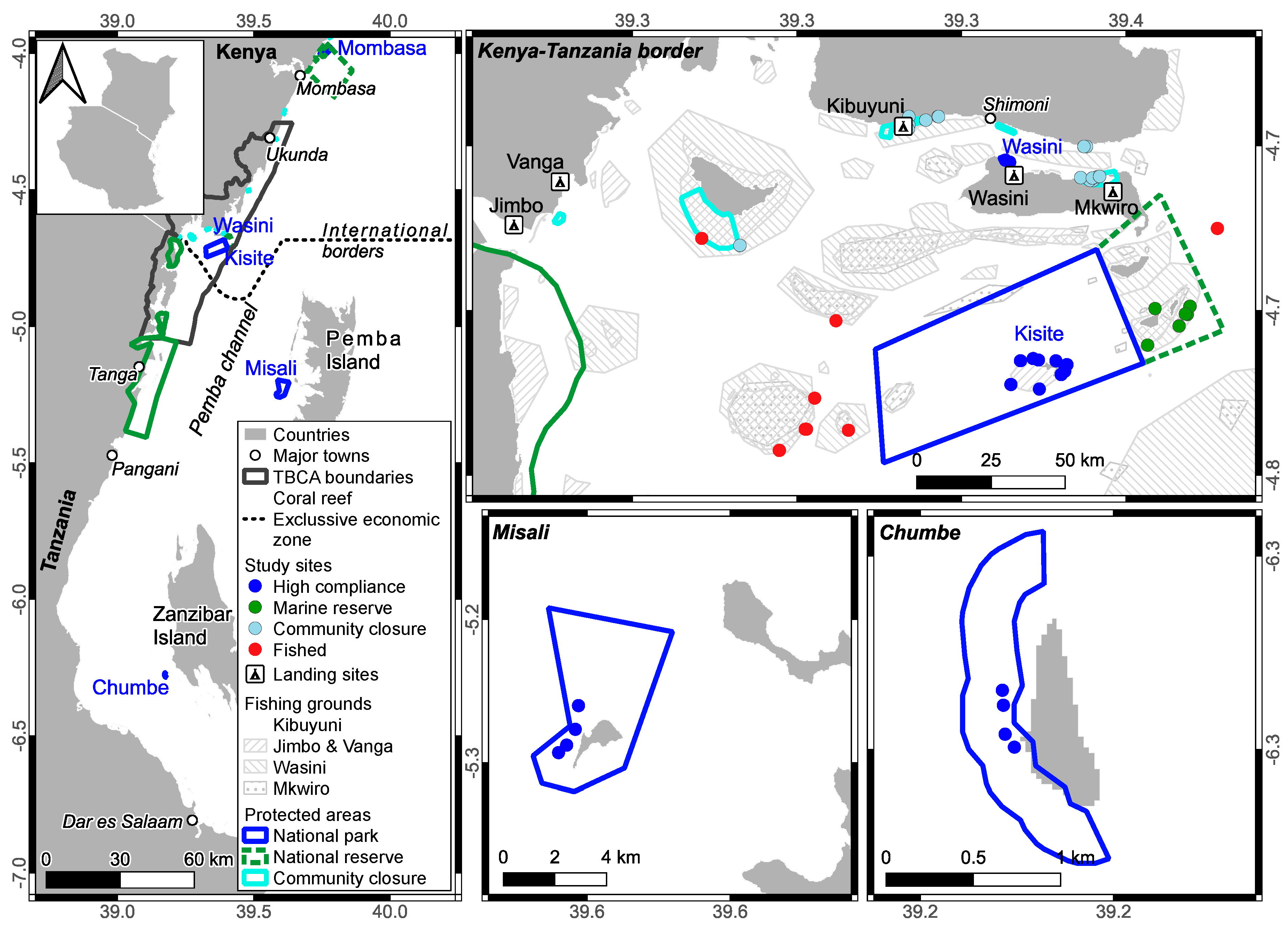
Figure 2. Plot of biomass as a function of time since closure to fishing in the 7 studied marine reserves showing the distribution among (a) marine reserve or fishing closure sites and (b) 12 “family/functional” taxonomic groupings summed to total biomass and presented as stacked bar graphs, pooling data at yearly interval. The zero-recovery time point is based on 14 adjacent fished study sites.

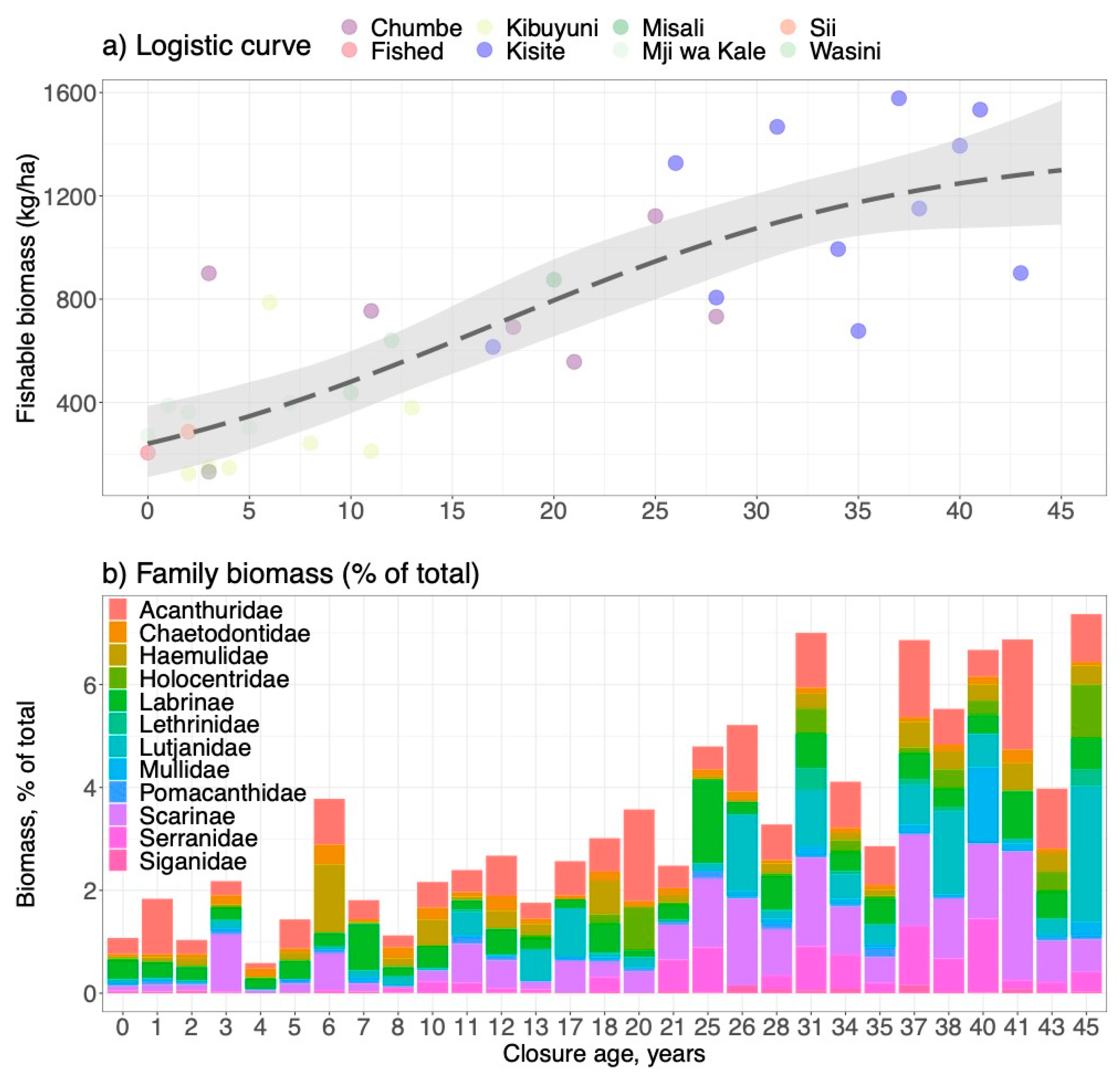
Figure 3. (a) Estimates of production (mean ± 1SEM) of the fish families as determined by the linear slope of the age of biomass recovery in 7 reserves (Supplementary Table S4b). (b) percent differences in biomass between the park and catch in the fisheries for the shared 12 sampled families/functional groups. The zero point represents no difference between park and fisheries biomass while negative values indicate higher biomass in the park than catch.

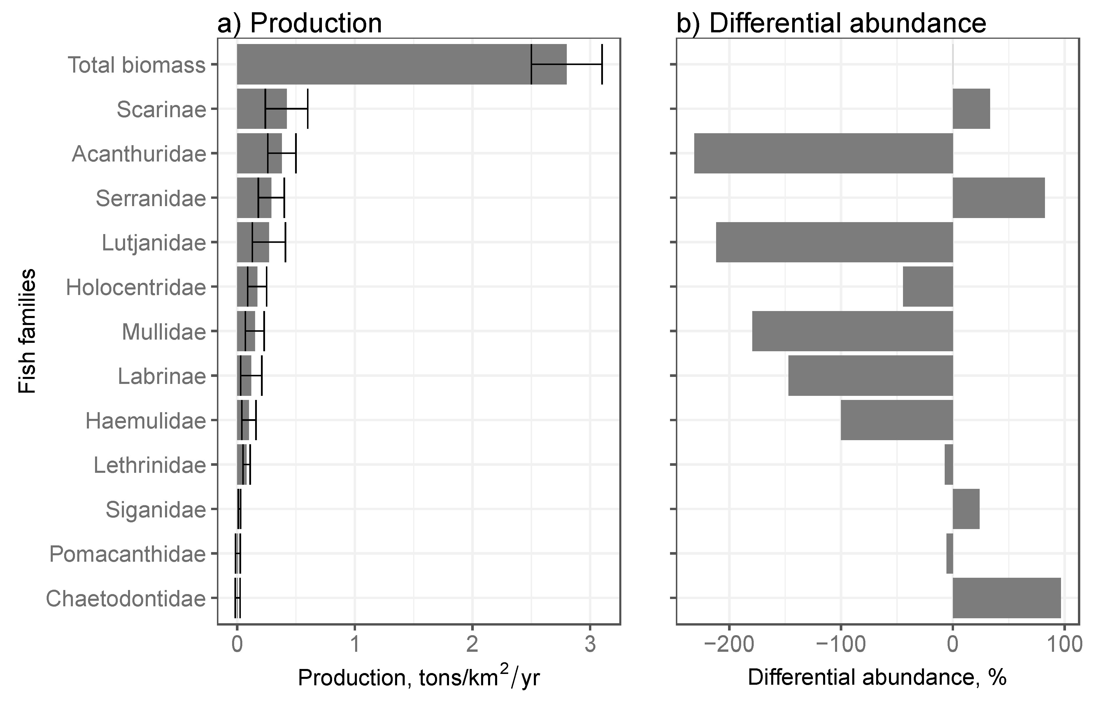
Figure 4. Plot of the cumulative number of species caught as a function of the cumulative number of individuals censused in the Kisite park and observed in each landing sites, marine reserve census and all fish landings (catch). Further, catch (all landing species pooled) and marine reserve species are presented as total, commercial, and home consumption categories. Data presented are based on all species observed or caught in 12 common family/functional groupings shared in the Kisite Marine reserve and fisheries at 5 landings sites respectively.

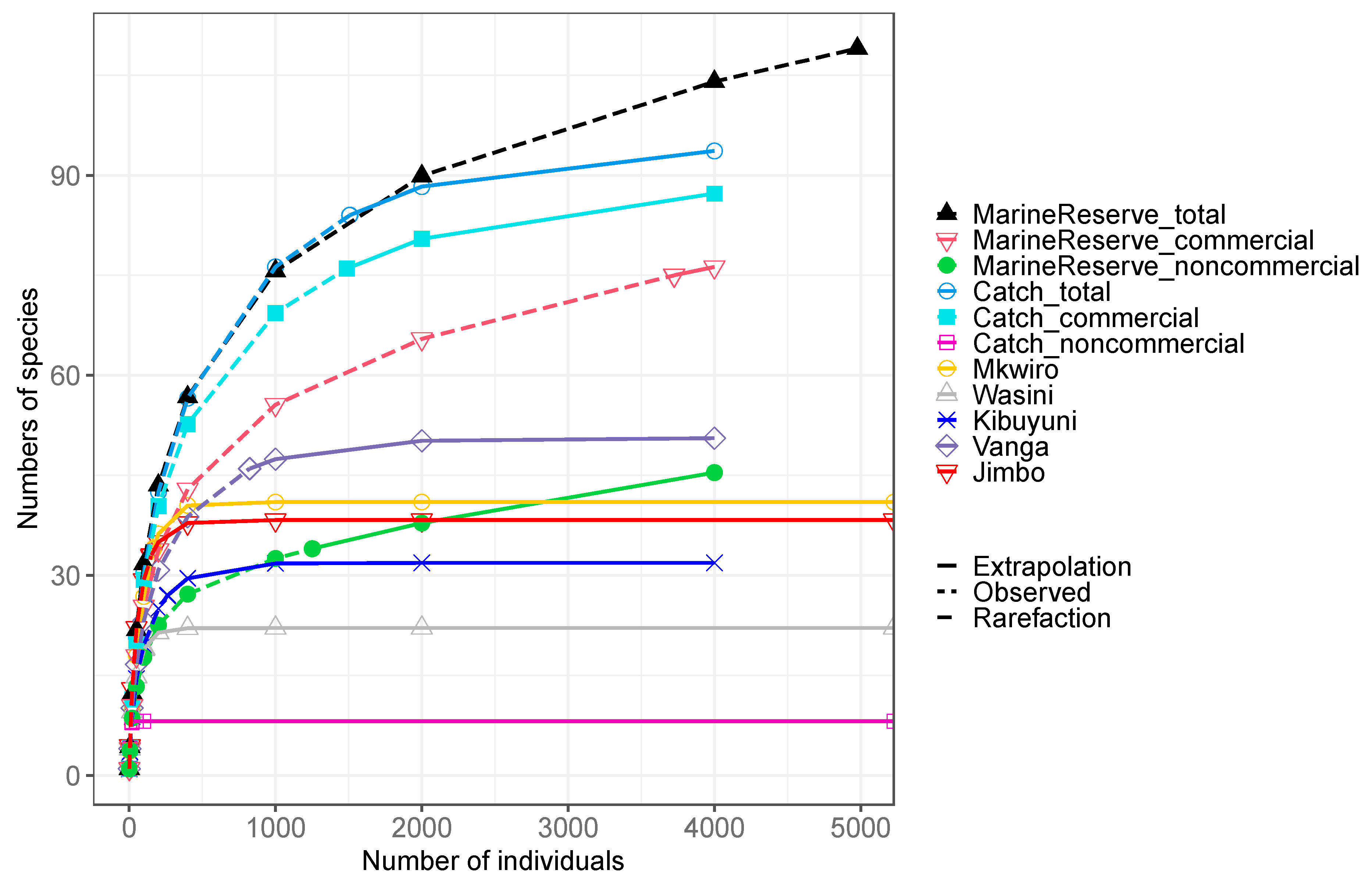
Figure 5. Ward hierarchical clusters of relative abundance of fish for (a) fish catch evaluated for fishing gears and (b) landed fish in the 5 landing sites and censused in the Kisite marine reserve. Multivariate Principal Component Analysis (PCA) with vectors of the relative abundance of fish as (c) catch by fishing gears and (d) landed in the 5 sites and censused in the Kisite marine reserve. Plots based on species contained within the 12 common families. List of species names associated with numbers is presented in Supplementary Table S5.

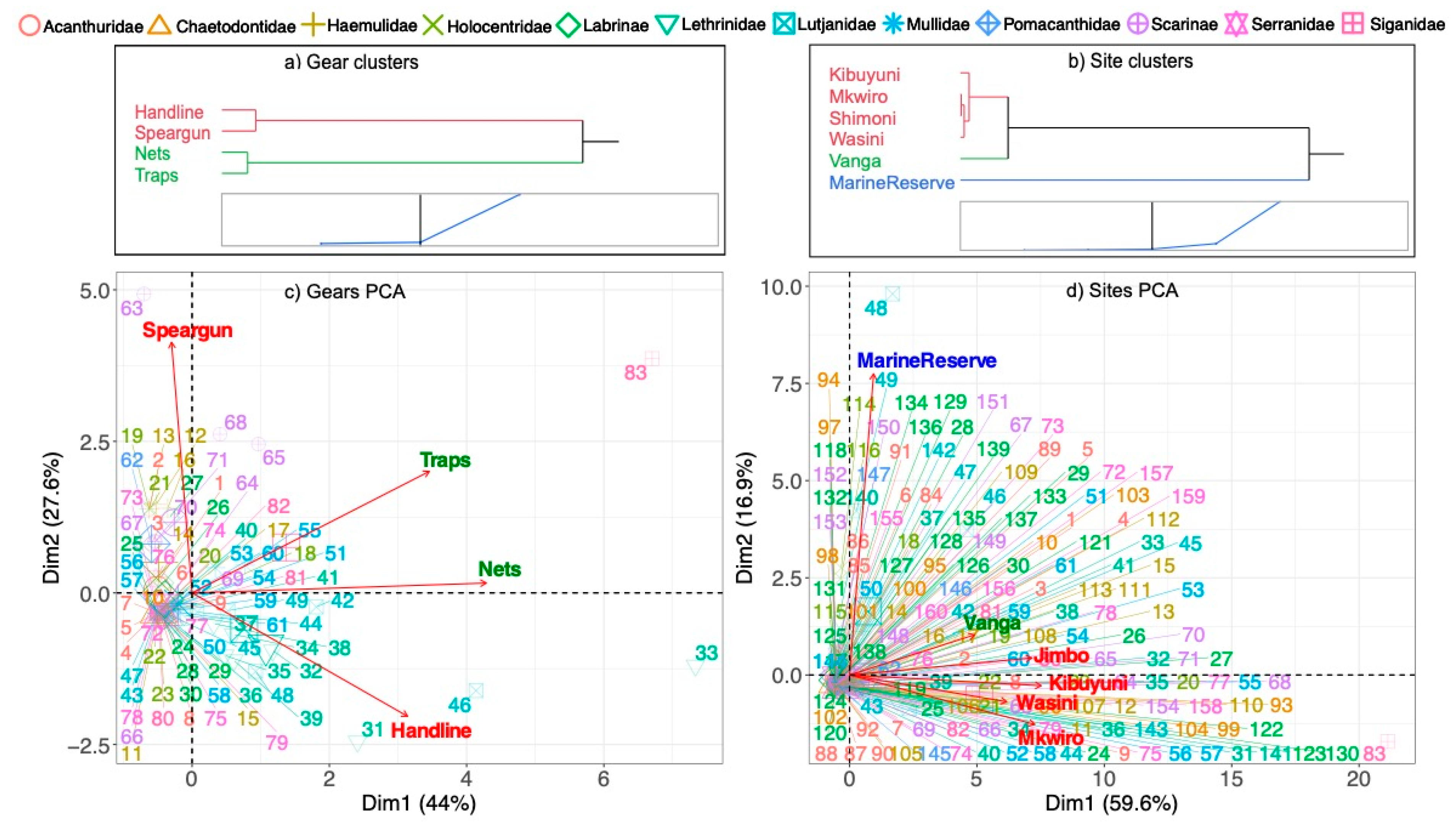
Figure 6. Summary plots of the catch relative to maximum sustained yield (Yield/MSY) at the 5 fishing villages for the relationships with (a) catch per unit effort (CPUE), (b) trophic level and natural mortality metrics, and (c) Shannon diversity indices of the catch.

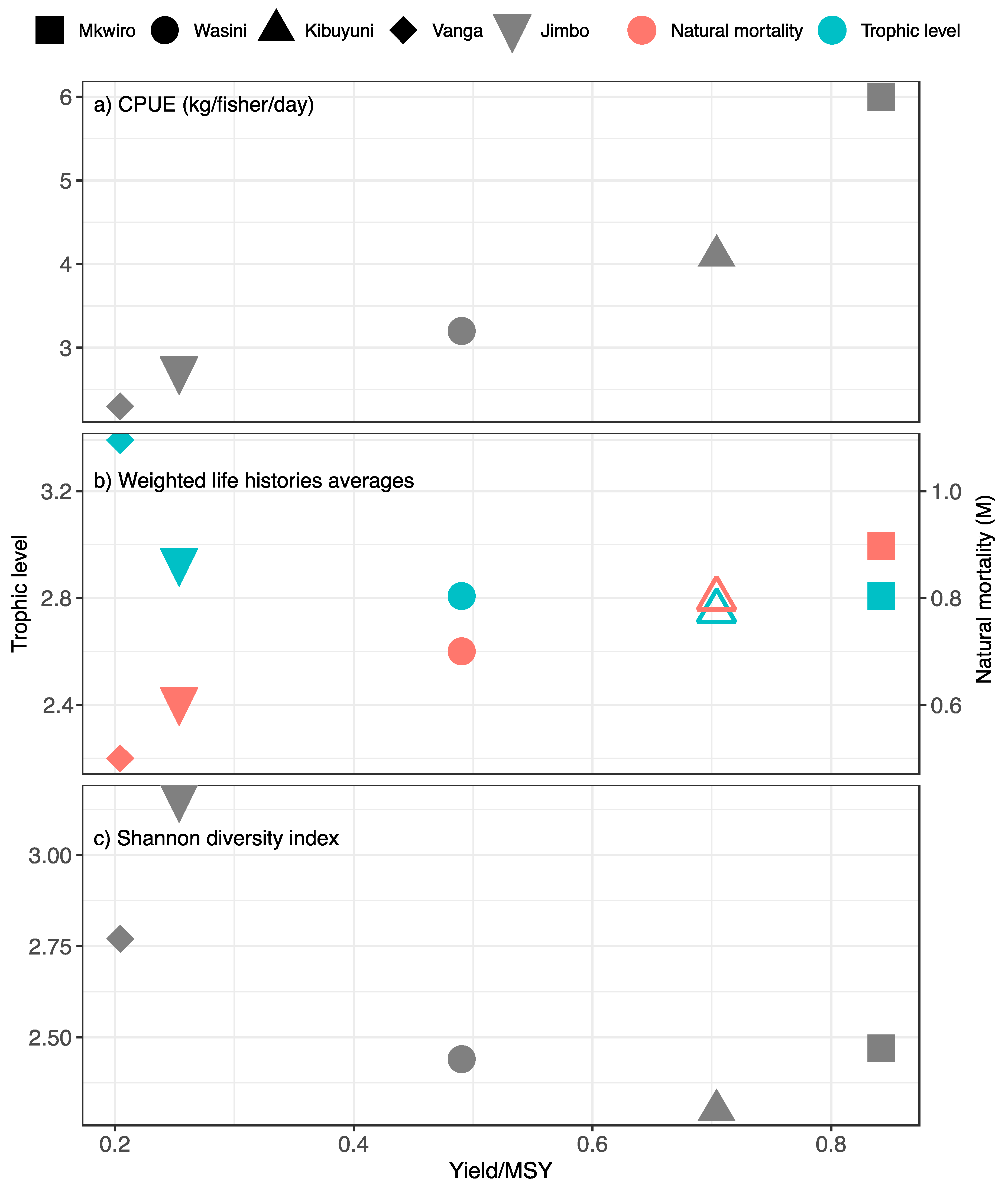
Figure 7. Summary of length and spawning potential based analyses showing species organized by families. Presented as the ratios of (a) length/length opt, (b) length/length mat, and (c) spawning potential ratio.

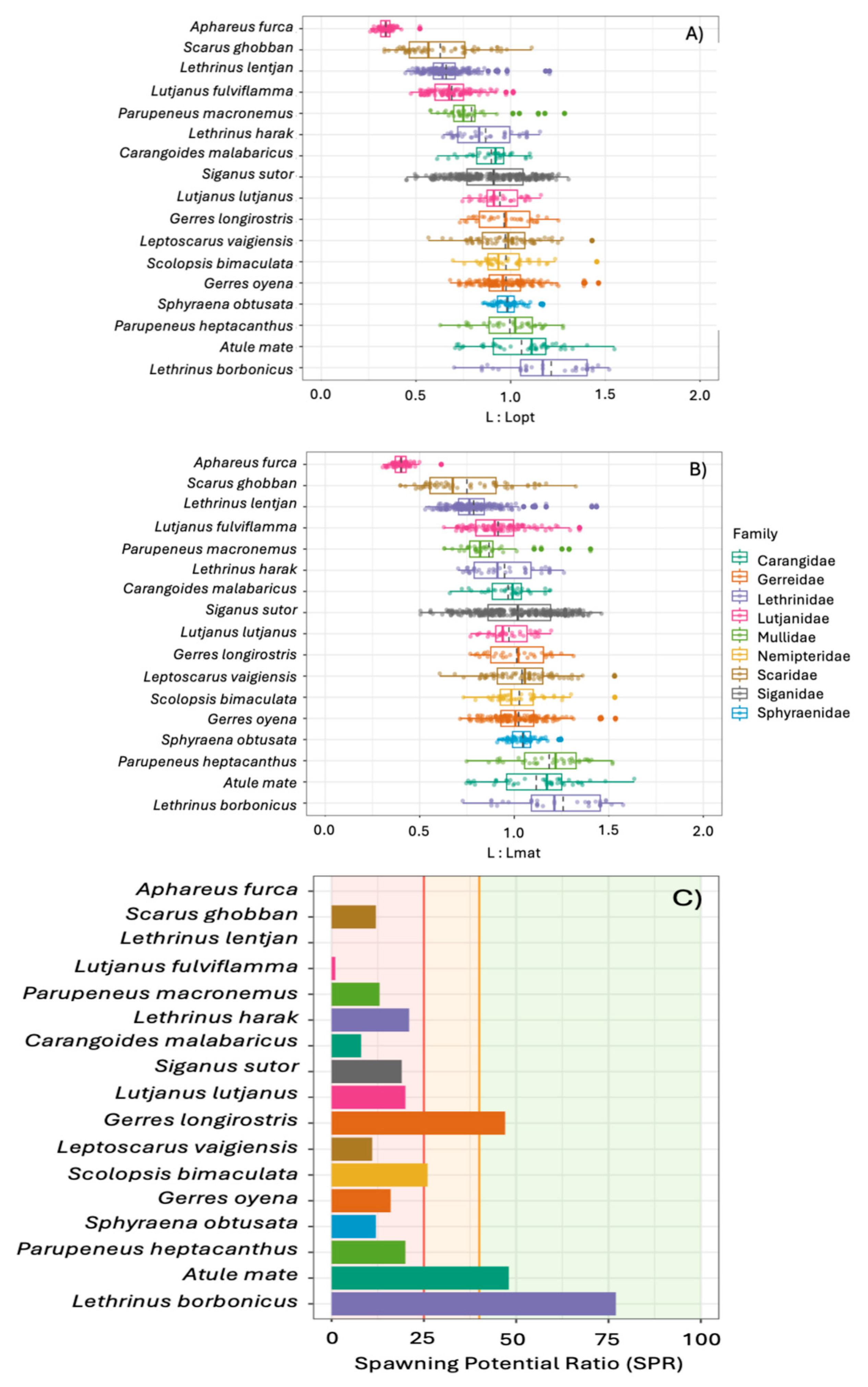
Table 1. Means and standard errors of the mean (± SE) statistics by site and all sites for catch collected over a 30 month-period for (a) sampling; sampled days per month, sample size, fishing effort (fishers/km²/day), catch-per-unit-effort (CPUE, kg/fisher/day), income (Ksh/fisher/day), yield (kg/km²/day), and yield (tons/km²/y). (b) Site and all sites CPUE, yield, and income for dominant fish groups. Kruskal-Wallis and post-hoc Dunn’s tests of significance are presented.

	Category	Mkwiro	Wasini	Kibuyuni	Vanga	Jimbo	ChiSq; Prob>ChiSq	All sites
a) Sampling	Days sampled/month	13.6 ± 0.9^a	11.5 ± 0.7^b	11.9 ± 0.7^b	11.7 ± 0.6^b	10.0 ± 0.6^c	17.1; 0.002	11.7 ± 0.3
	Sample size (n)	366	320	345	318	286		1635
	Effort (Fishers/km²/day)	2.06 ± 0.16^a	1.85 ± 0.1^a	2.56 ± 0.28^b	1.29 ± 0.06^c	1.15 ± 0.08^c	63.6; <0.0001	1.77 ± 0.08
	CPUE (kg/fisher/day)	5.58 ± 0.28^a	3.46 ± 0.24^b	4.11 ± 0.2^b	2.4 ± 0.08^c	3.51 ± 0.21^b	75.0; <0.0001	3.79 ± 0.13
	Income (Ksh/fisher/day)	1214.76 ± 56.06^a	920.43 ± 66.62^b	841.12 ± 40.59^b	374.14 ± 17.58^c	548.89 ± 37.03^c	94.7; <0.0001	772.27 ± 32.03
	Yield (kg/km²/day)	11.95 ± 1.35^a	6.96 ± 0.69^b	9.99 ± 0.91^b	2.9 ± 0.17^c	3.6 ± 0.19^c	90.2; <0.0001	6.99 ± 0.45
	Yield (tons/km²/y)	2.53 ± 0.29^a	1.48 ± 0.15^b	2.12 ± 0.19^b	0.62 ± 0.04	0.76 ± 0.04^c	90.2; <0.0001	1.48 ± 0.10
b) Fish groups
CPUE	Goatfish	0.13 ± 0.01^a	0.06 ± 0.01^b	0.11 ± 0.02^b	0.04 ± 0.01^c	0.01 ± 0.004c	70.4; <0.0001	0.07 ± 0.01^a
	Mixed catch	0.43 ± 0.04^a	0.25 ± 0.02^c	0.19 ± 0.01^c	0.60 ± 0.07^a	0.76 ± 0.09^b	68.7; <0.0001	0.44 ± 0.03^b
	Octopus	0.21 ± 0.03^a	0.22 ± 0.03^a	0.39 ± 0.03^a	0.30 ± 0.03^a	0.97 ± 0.09^b	59.4; <0.0001	0.41 ± 0.03^b
	Parrotfish	0.28 ± 0.02^a	0.20 ± 0.03^b	0.17 ± 0.02^b	0.15 ± 0.03^b	0.10 ± 0.02^b	26.8; <0.0001	0.18 ± 0.01^c
	Pelagics	0.20 ± 0.03^a	0.26 ± 0.04^a	0.17 ± 0.03^a	0.60 ± 0.08^b	0.46 ± 0.08^b	42.3; <0.0001	0.34 ± 0.03^d
	Rabbitfish	0.58 ± 0.07^a	0.40 ± 0.04^b	0.33 ± 0.02^c	0.23 ± 0.04^c	0.33 ± 0.08^c	32.7; <0.0001	0.37 ± 0.03^b
	Scavengers	0.50 ± 0.03^a	0.33 ± 0.03^a	0.22 ± 0.02^b	0.97 ± 0.11^c	0.61 ± 0.09^a	51.3; <0.0001	0.52 ± 0.04^e
Yield	Goatfish	0.11 ± 0.02^a	0.03 ± 0.01^b	0.06 ± 0.01^b	0.01 ± 0.002^c	0.003 ± 0.002^c	88.5; <0.0001	0.04 ± 0.01^a
	Mixed catch	0.42 ± 0.07^a	0.16 ± 0.02^b	0.17 ± 0.03^b	0.32 ± 0.04^c	0.25 ± 0.03^c	22.0; 0.0002	0.27 ± 0.02^b
	Octopus	0.07 ± 0.01^a	0.10 ± 0.02^a	0.38 ± 0.07^b	0.17 ± 0.02^a	0.47 ± 0.05^b	62.9; <0.0001	0.24 ± 0.02^b
	Parrotfish	0.25 ± 0.04^a	0.11 ± 0.02^b	0.15 ± 0.02^b	0.05 ± 0.01^c	0.04 ± 0.01^c	55.5; <0.0001	0.12 ± 0.01^c
	Pelagics	0.09 ± 0.02^a	0.22 ± 0.05^a	0.13 ± 0.04^a	0.34 ± 0.02^b	0.23 ± 0.04^a	42.2; <0.0001	0.20 ± 0.02^d
	Rabbitfish	0.60 ± 0.09^a	0.45 ± 0.07^a	0.54 ± 0.06^a	0.05 ± 0.01^b	0.08 ± 0.02^b	85.3; <0.0001	0.34 ± 0.03^e
	Scavengers	0.52 ± 0.04^a	0.32 ± 0.03^a	0.31 ± 0.06^a	0.12 ± 0.02^b	0.17 ± 0.02^b	50.2; <0.0001	0.29 ± 0.02^b
Income	Goatfish	29.66 ± 3.00^a	17.57 ± 2.80^a	22.75 ± 2.90^a	6.98 ± 2.34^b	1.95 ± 0.81^b	74.1; <0.0001	15.79 ± 1.41^a
	Mixed catch	71.87 ± 7.16^a	51.47 ± 4.83^a	26.65 ± 2.05^b	68.33 ± 7.22^a	81.17 ± 8.89^c	46.9; <0.0001	59.53 ± 3.28^b
	Octopus	49.35 ± 6.65^a	61.73 ± 8.09^b	97.15 ± 7.76^c	72.59 ± 7.82^b	184.25 ± 20.38^d	49.3; <0.0001	92.30 ± 6.37^c
	Parrotfish	49.89 ± 4.77^a	47.00 ± 6.02^a	25.25 ± 2.49^b	23.81 ± 4.90^c	11.45 ± 2.74^c	46.9; <0.0001	31.35 ± 2.30^a
	Pelagics	47.64 ± 7.07^a	69.25 ± 10.44^a	39.00 ± 6.28^a	85.86 ± 12.96^b	77.94 ± 14.69^a	14.4; 0.006	63.93 ± 4.99^b
	Rabbitfish	149.99 ± 19.75^a	114.39 ± 10.77^a	70.18 ± 4.69^b	51.49 ± 10.02^b	64.34 ± 16.48^b	45.1; <0.0001	88.61 ± 6.57^c
	Scavengers	118.19 ± 8.67^a	92.50 ± 8.79^a	44.39 ± 4.87^b	168.2 ± 17.56^c	87.20 ± 12.90^a	48.2; <0.0001	100.84 ± 6.04^c

Table 2. Numbers of unique species caught by gear, site, and totals. Means and standard errors of the mean (± SE) and sample sizes by site, gear, and total for (b) fish length measured nearest to millimeter, (c) catch-per-unit-effort (CPUE, kg/fisher/day), (d) yield (kg/km²/day), and income (Ksh/fisher/day). Kruskal-Wallis and post-hoc Dunn’s tests of significance are presented.

	Category	Mkwiro (n)	Wasini (n)	Kibuyuni (n)	Vanga (n)	Jimbo (n)	ChiSq; Prob>ChiSq	All sites (n)
a) Number of species	Traps	30	16	28	32	22		66
	Speargun	0	5	0	7	20		27
	Handline	8	0	15	9	9		29
	Nets	0	2	6	88	5		93
	All gears	34	21	30	104	43
b) Fish length	Traps	28.0 ± 0.5 (151) ^a	25.0 ± 0.8 (63)^b	27.0 ± 0.4 (178) ^b	22.0 ± 0.4 (226) ^c	28.0 ± 0.8 (100) ^b	120.6; <0.0001	26.0 ± 0.3 (718) ^b
	Speargun		24.0 ± 1.1 (15)^a		23.0 ± 1.0 (11)^a	26.0 ± 1.5 (33)^a	NS	25.0 ± 0.9 (59)^b
	Handline	19.0 ± 0.8 (15)^a	34.0 ± 1.0 (6)^b	20.0 ± 1.0 (58)^a	20.0 ± 0.4 (37)^a	22.0 ± 1.1 (23)^b	18.8; 0.0009	21.0 ± 0.5 (139) ^a
	Nets		19.0 ± 0.2 (20)^a	26.0 ± 0.7 (33)^b	19.0 ± 0.2 (840) ^a	19.0 ± 0.9 (10)^a	27.6; <0.0001	19.0 ± 0.2 (903) ^a
	All gears	28.0 ± 0.5 (166) ^a	24.0 ± 0.6 (104) ^b	25.0 ± 0.4 (269) ^a	20.0 ± 0.2 (1114) ^c	26.0 ± 0.6 166) ^a	292.5; <0.0001	22.0 ± 0.2 (1819)
c) CPUE	Traps	5.45 ± 0.33^a	3.41 ± 0.27^b	4.47 ± 0.23^a	6.94 ± 0.51^c	4.85 ± 0.37^a	46.1; <0.0001	5.05 ± 0.19^a
	Speargun	3.93 ± 0.37^a	3.28 ± 0.23^a	3.34 ± 0.18^a	3.41 ± 0.23^a	3.73 ± 0.21^a	NS	3.51 ± 0.11^b
	Handline	5.1 ± 0.31^a	2.82 ± 0.27^a	3.48 ± 0.24^a	3.38 ± 0.34^a	2.84 ± 0.17^b	35.9; <0.0001	3.52 ± 0.14^b
	Nets	3.25 ± 0.46^a	4.08 ± 0.3^b	4.16 ± 0.4^c	3.18 ± 0.24^b	2.88 ± 0.26^c	16.9; 0.002	3.48 ± 0.14^c
	All gears	4.64 ± 0.2^a	3.61 ± 0.17^b	3.82 ± 0.15^b	3.8 ± 0.19^b	3.37 ± 0.15^b	33.7; <0.0001	3.77 ± 0.08
d) Yield	Traps	6.93 ± 1.07^a	3.35 ± 0.43^b	4.92 ± 0.49^c	0.67 ± 0.05^d	1.09 ± 0.14^d	87.6; <0.0001	3.39 ± 0.32^a
	Speargun	1.05 ± 0.1^a	0.99 ± 0.09^a	2.74 ± 0.33^b	1.37 ± 0.13^a	1.5 ± 0.15^a	26.5; <0.0001	1.59 ± 0.1^c
	Handline	3.71 ± 0.44^a	1.17 ± 0.15^b	2.2 ± 0.39^c	0.29 ± 0.04^d	0.62 ± 0.06^d	69.6; <0.0001	1.68 ± 0.17^b
	Nets	1.08 ± 0.13^a	2.66 ± 0.23^b	3.25 ± 0.48^b	1.08 ± 0.06^a	1.55 ± 0.14^a	51.7; <0.0001	1.87 ± 0.1^c
	All gears	3.52 ± 0.42^a	2.16 ± 0.15^b	3.21 ± 0.22^a	0.99 ± 0.04^c	1.3 ± 0.08^c	130.6; <0.0001	2.04 ± 0.08
e) Income	Traps	1215.04 ± 68.75^a	916.15 ± 77.57^b	873.11 ± 46.77^b	1030.59 ± 68.24^b	715.65 ± 64.23^c	29.1; <0.0001	955.8 ± 32.25^a
	Speargun	924.93 ± 88.34^a	892.86 ± 66.6^a	718.03 ± 36.75^a	746.13 ± 45.79^a	692.56 ± 47.84^a	NS	790.39 ± 26.45^c
	Handline	1093.29 ± 63.82^a	736.76 ± 72.45^b	674.35 ± 47.23^b	605.34 ± 90.25^b	366.21 ± 20.29^c	58.9; <0.0001	697.55 ± 33.7^b
	Nets	686.99 ± 109.17^a	1056.5⁴ ± 80.74^b	822.24 ± 85.34^b	491.23 ± 44.39^a	436.81 ± 49.46^a	70.8; <0.0001	678.73 ± 34.34^d
	All gears	1033.58 ± 43.59^a	950.76 ± 44.63^a	769.32 ± 29.64^b	622.49 ± 33.58^c	529.5 ± 28.53^c	126.5; <0.0001	757.29 ± 17.91

Table 3. Simpson’s, Shannon-Weiner, and Evenness diversity indices for (a) dominant gears, and (b) study sites. Gears summaries were compiled from all species identified in 12 common families in catch landing data. Sites summaries were compiled from all species identified in 12 common families during both catch and field sampling.

a) Gears	Simpson’s index	Shannon index	Evenness
Speargun	0.93	2.86	1.0
Traps	0.82	2.67	0.93
Nets	0.88	2.61	0.91
Handline	0.90	2.55	0.89
b) Sites
Marine reserve	0.92	3.27	1.0
Jimbo	0.94	3.15	0.97
Vanga	0.88	2.77	0.85
Mkwiro	0.81	2.47	0.76
Wasini	0.87	2.44	0.75
Kibuyuni	0.79	2.30	0.70

Table 4. Summaries of common (a) families and (b) species abundance (mean ± standard deviation, SD) and sample size (n) of fish landing sampling at 5 sites (catch landing) and field sampling using discrete group sampling (DGS) transects in Marine National Park (MNP). Species are based on the 40 species in common in the census and fish landing data. Percentages of total and coefficients of variations (COV, %) for catch landing and field sampling are presented as well as percentage differential abundance between catch and field sampling of the unfished Kisite marine reserve [(catch%-reserve%)/catch%*100]. Simpson’s dominance, Shannon diversity, and Evenness indices are presented for family and species. Table ordered from most negative to most positive differential abundances.

	Fish landing sampling			Field sampling (DGS)
a) Family	Numbers/fishing group/day ± SD (n)	Percentage of total	COV, %	Numbers/500m² ± SD (n)	Percentage of total	COV, %	Differential abundance, %
Acanthuridae	0.01 ± 0.11 (12)	1.6	1928.8	3.38 ± 7.62 (152)	5.3	225.7	-231.3
Lutjanidae	0.03 ± 0.40 (13)	1.7	1277.2	17.11 ± 19.59 (154)	5.3	114.5	-211.8
Mullidae	0.09 ± 0.65 (192)	25.5	699.9	45.56 ± 133.93 (2050)	71.2	294	-179.2
Labrinae	0.01 ± 0.13 (13)	1.7	1622	3.33 ± 12.41 (120)	4.2	372.4	-147.1
Haemulidae	0.005 ± 0.10 (2)	0.3	2032.2	2.0 ± 1.8 (18)	0.6	90.1	-100
Holocentridae	0.01 ± 0.13 (7)	0.9	1588	2.11 ± 3.63 (38)	1.3	171.9	-44.4
Lethrinidae	0.01 ± 0.10 (20)	2.7	1419.3	1.33 ± 2.37 (84)	2.9	177.7	-7.4
Pomacanthidae	0.02 ± 0.25 (27)	3.6	1169.5	4.07 ± 7.98 (110)	3.8	195.8	-5.6
Siganidae	0.01 ± 0.01 (16)	2.1	100	1.0 ± 1.57 (45)	1.6	156.7	23.8
Scarinae	0.005 ± 0.07 (2)	0.3	1435.3	0.56 ± 0.73 (5)	0.2	130.8	33.3
Serranidae	0.04 ± 0.37 (89)	11.8	865.4	1.33 ± 1.82 (60)	2.1	136.6	82.2
Chaetodontidae	0.87 ± 2.04 (360)	47.8	234.3	5.0 ± 11.63 (45)	1.6	232.6	96.7
Simpson’s index	0.69			0.48
Shannon index	1.53			1.16
Evenness	1			0.76
b) Species
Gomphosus caeruleus	0.049 ± 0.002 (1)	0.1	4.9	5.6 ± 3.5 (50)	1.74	63.7	-1640
Lutjanus kasmira	0.46 ± 0.05 (20)	2.7	10.5	124.2 ± 250.7 (1118)	38.81	201.8	-1337.4
Lutjanus gibbus	0.049 ± 0.002 (1)	0.1	4.9	4.3 ± 8.9 (39)	1.35	205.1	-1250
Naso annulatus	0.098 ± 0.005 (2)	0.3	4.9	12.4 ± 13.8 (112)	3.89	110.6	-1196.7
Myripristis berndti	0.139 ± 0.01 (4)	0.5	7	11.7 ± 23.8 (105)	3.64	203.8	-628
Mulloidichthys vanicolensis	0.148 ± 0.01 (3)	0.4	4.9	6.8 ± 13.3 (61)	2.12	195.7	-430
Ctenochaetus striatus	0.049 ± 0.002 (1)	0.1	4.9	1.4 ± 1.7 (13)	0.45	120.5	-350
Aethaloperca rogaa	0.049 ± 0.002 (1)	0.1	4.9	1.2 ± 1.4 (11)	0.38	114.1	-280
Lutjanus lutjanus	0.462 ± 0.08 (35)	4.6	18.3	53.3 ± 138.9 (480)	16.66	260.5	-262.2
Cephalopholis argus	0.098 ± 0.005 (2)	0.3	4.9	3.2 ± 1.8 (29)	1.01	55.5	-236.7
Lethrinus obsoletus	0.402 ± 0.03 (13)	1.7	7.8	17.1 ± 19.6 (154)	5.35	114.5	-214.7
Scarus frenatus	0.07 ± 0.005 (2)	0.3	7	2.4 ± 2.0 (22)	0.76	82.1	-153.3
Plectorhinchus gaterinus	0.12 ± 0.01 (4)	0.5	8.1	4.0 ± 4.4 (36)	1.25	111.1	-150
Chaetodon auriga	0.098 ± 0 (2)	0.3	4.9	2.0 ± 1.8 (18)	0.62	90.1	-106.7
Thalassoma lunare	0.049 ± 0 (1)	0.1	4.9	0.6 ± 0.7 (5)	0.17	130.8	-70
Halichoeres hortulanus	0.085 ± 0.01 (3)	0.4	8.5	2.1 ± 1.7 (19)	0.66	80.1	-65
Acanthurus leucosternon	0.148 ± 0.01 (3)	0.4	4.9	1.9 ± 2.9 (17)	0.59	155.4	-47.5
Parupeneus barberinus	0.322 ± 0.03 (13)	1.7	9.8	5.3 ± 1.7 (48)	1.67	32.5	1.8
Lutjanus fulviflamma	0.824 ± 0.28 (116)	15.4	34.1	45.8 ± 71.9 (412)	14.3	157.1	7.1
Acanthurus nigricauda	0.07 ± 0.005 (2)	0.3	7	0.8 ± 1.0 (7)	0.24	124.9	20
Sargocentron caudimaculatum	0.098 ± 0.005 (2)	0.3	4.9	0.8 ± 1.6 (7)	0.24	201	20
Scarus psittacus	0.13 ± 0.01 (5)	0.7	9.3	1.7 ± 1.8 (15)	0.52	108.2	25.7
Pomacanthus imperator	0.07 ± 0.005 (2)	0.3	7	0.6 ± 0.7 (5)	0.17	130.8	43.3
Myripristis murdjan	0.148 ± 0.01 (3)	0.4	4.9	0.4 ± 1.0 (4)	0.14	228.1	65
Calotomus carolinus	0.36 ± 0.04 (16)	2.1	10.8	2.1 ± 2.2 (19)	0.66	104.4	68.6
Anampses caeruleopunctatus	0.049 ± 0.002 (1)	0.1	4.9	0.1 ± 0.3 (1)	0.03	300	70
Bodianus bilunulatus	0.049 ± 0.002 (1)	0.1	4.9	0.1 ± 0.3 (1)	0.03	300	70
Epinephelus spilotoceps	0.049 ± 0.002 (1)	0.1	4.9	0.1 ± 0.3 (1)	0.03	300	70
Cheilinus trilobatus	0.098 ± 0.01 (4)	0.5	9.9	0.4 ± 0.5 (4)	0.14	118.6	72
Sargocentron diadema	0.12 ± 0.01 (4)	0.5	8.1	0.4 ± 1.0 (4)	0.14	228.1	72
Acanthurus dussumieri	0.155 ± 0.01 (4)	0.5	6.2	0.3 ± 0.7 (3)	0.1	212.1	80
Plectorhinchus flavomaculatus	0.148 ± 0.01 (3)	0.4	4.9	0.2 ± 0.4 (2)	0.07	198.4	82.5
Cheilio inermis	0.202 ± 0.02 (9)	1.2	10.8	0.4 ± 0.7 (4)	0.14	163.5	88.3
Epinephelus merra	0.07 ± 0.005 (2)	0.3	7	0.1 ± 0.3 (1)	0.03	300	90
Cephalopholis boenak	0.26 ± 0.02 (10)	1.3	9.3	0.3 ± 0.5 (3)	0.1	150	92.3
Scarus rubroviolaceus	0.109 ± 0.01 (5)	0.7	11.1	0.1 ± 0.3 (1)	0.03	300	95.7
Siganus sutor	2.042 ± 0.87 (360)	47.8	42.7	5.0 ± 11.6 (45)	1.56	232.6	96.7
Parupeneus cyclostomus	0.264 ± 0.03 (11)	1.5	10.1	0.1 ± 0.3 (1)	0.03	300	98
Scarus ghobban	0.721 ± 0.15 (61)	8.1	20.5	0.3 ± 1.0 (3)	0.1	300	98.8
Lutjanus argentimaculatus	0.984 ± 0.05 (20)	2.7	4.9	0.1 ± 0.3 (1)	0.03	300	98.9
Simpson’s index	0.74			0.79
Shannon index	2.09			2.16
Evenness	0.96			1.0

Table 5. Weighted averages of life history traits for negative and positive differential abundance based on species in the categories of (a) sampling groups namely catch, marine reserve, shared common species and all species and (b) fishing gears.

a) Sampling group	Differential Category	Number of species	Trophic level	Growth rate (K/year)	Natural mortality (M)	Life span	Generation time	Age at first maturity ™	Length at maturity (Lmat)	Length at MSY (Lopt)	Maximum length (Lmax)
Catch	Negative	32	3.6	0.6	0.4	7.6	2.3	1.8	25.0	28.1	55.1
	Positive	11	2.3	1.1	1.2	5.9	1.7	1.4	21.8	23.4	39.7
Marine reserve	Negative	45	2.3	0.5	0.8	7.8	2.4	2.0	16.0	16.5	27.5
	Positive	24	2.9	1.0	1.2	4.3	1.5	1.2	15.2	13.5	29.3
Species shared in common	Negative	28	3.8	0.4	0.6	9.2	2.7	2.3	21.2	23	42.8
	Positive	12	2.5	0.6	1.0	5.6	1.7	1.4	27.1	30.6	48.8
All species	Negative	105	3.2	0.5	0.6	8.2	2.5	2	20.7	22.5	41.8
	Positive	47	1.7	0.7	0.8	3.4	1.1	0.9	12.4	12.3	23
b) Fishing gears	Nets	90	3.1	0.7	1.1	5.8	1.8	1.4	25.9	29.8	54.7
	Traps	65	2.8	0.6	0.8	6.7	2.0	1.6	25.2	28.1	48.0
	Handline	29	3.7	0.5	0.5	8.0	2.3	1.9	22.7	25.2	49.6
	Speargun	27	2.6	0.4	0.7	8.4	2.5	2.0	28.1	32.0	52.3
	All gears	211	3.05	0.55	0.78	7.3	2.15	1.73	25.48	28.78	51.2

Disclaimer/Publisher’s Note: The statements, opinions and data contained in all publications are solely those of the individual author(s) and contributor(s) and not of MDPI and/or the editor(s). MDPI and/or the editor(s) disclaim responsibility for any injury to people or property resulting from any ideas, methods, instructions or products referred to in the content.

© 2024 by the authors. Licensee MDPI, Basel, Switzerland. This article is an open access article distributed under the terms and conditions of the Creative Commons Attribution (CC BY) license (http://creativecommons.org/licenses/by/4.0/).

Copyright: This open access article is published under a Creative Commons CC BY 4.0 license, which permit the free download, distribution, and reuse, provided that the author and preprint are cited in any reuse.

Downloads

126

Views

Comments

Subscription

Notify me about updates to this article or when a peer-reviewed version is published.

MDPI Initiatives

Important Links

Choose an area of interest and we will send you notifications of new preprints at your preferred frequency.

Disclaimer