Preliminary Exploration on Short-Term Prediction of Local Geomagnetically Induced Currents Using Hybrid Neural Networks

Preprint

Article

Preliminary Exploration on Short-Term Prediction of Local Geomagnetically Induced Currents Using Hybrid Neural Networks

This version is not peer-reviewed.

Yihao Fang,

Jin Liu^*

,Haiyang Jiang,Wenhao Chen

Yihao Fang,

Jin Liu^*

,Haiyang Jiang,Wenhao Chen

This version is not peer-reviewed.

Altmetrics

Downloads

Views

Comments

Submitted:

31 October 2024

Posted:

01 November 2024

You are already at the latest version

A peer-reviewed article of this preprint also exists.

Abstract

During extreme space weather events, transient geomagnetic disturbances initiated by solar eruptive activities can induce geomagnetically induced currents (GICs), which have severe impacts on power grid systems and oil/gas pipelines. Observations indicate that GICs in power grids are characterized by large fluctuation amplitudes, broad frequency ranges, and significant randomness. Their behavior is influenced by several factors, including the sources of space weather disturbance, Earth's electrical conductivity distribution, the structural integrity and performance of power grid equipment, and so on. Consequently, predicting local grid GICs has been a highly challenging task. This paper presents a hybrid prediction approach using actual GIC data from power grids and deep learning techniques. We employ various technical methods, including Complete Ensemble Empirical Mode Decomposition with Adaptive Noise (CEEMDAN), Convolutional Neural Networks (CNN), Long Short-Term Memory Networks (LSTM), and Attention mechanisms, to investigate short-term prediction methods for local grid GICs. The study uses GIC monitoring samples from November 8th to November 10th, 2004, for model training and testing. The results are evaluated using the coefficient of determination R^2 , root mean square error (RMSE), and mean absolute error (MAE). Preliminary research suggests that the CEEMDAN-CNN-LSTM-Attention combined model significantly improves prediction accuracy and reduces the time delay in GIC prediction during geomagnetic storms compared to using LSTM neural networks alone.

Keywords:

Subject:

Environmental and Earth Sciences - Geophysics and Geology

1. Introduction

Eruptions of intense solar activity result in the ejection of hundreds of millions of tons of ultra-high temperature plasma from coronal active regions. This plasma disperses with the solar wind, forming coronal mass ejections (CMEs) [1]. When a CME approaches near-Earth space and interacts with the Earth’s magnetosphere, it induces a significant global disturbance in the geomagnetic field, known as a geomagnetic storm. The resulting magnetic field perturbation generates an induced electric field in the Earth’s crust, which in turn drives geomagnetically induced currents (GICs) in artificial conductive systems [2]. These GICs pose substantial threats to large artificial conductive technical infrastructure, such as power grids and oil- or gas- pipelines.

Following the Quebec incident in Canada in 1989 [3], the potential threat of extreme space weather to high-latitude power grids has been widely concerned. After the Halloween geomagnetic storm events in 2003 [4], power grids in mid- and low- latitude countries, including China, Australia, New Zealand, and Brazil, reported significant GIC phenomena. Notably, during the intense geomagnetic storm in November 2004, studies indicated that the GIC risk at the grounded neutral point of some transformers at the Lingao Nuclear Power Station in China reached 75.5A [6]. This current amplitude significantly exceeds the operational stability threshold for transformers, warranting the attention of power grid authorities.

Early theoretical research on geomagnetically induced currents (GICs) is exemplified by the plane wave model developed by Pirjola et al. [7] and the complex image method by Boteler et al. [8]. Expanding upon these foundational works, Viljanen et al. [9] introduced a suite of rapid calculation methods for space currents, aligning with the equivalent current system theory. Ngwira et al. [10] improved the traditional plane wave algorithm by incorporating a layered geoelectric conductivity model, subsequently applying this refined model to investigate GICs within the South African power grid. Simultaneously, empirical GIC prediction models have been formulated, utilizing local satellite observations of the interplanetary solar wind at 1 AU, along with solar wind parameters and geomagnetic field data as inputs [11]. These models have enabled comprehensive statistical analyses, examining the relationships between GIC intensity, frequency, site latitudes, voltage levels, and line orientations.

For a long time, due to the lack of direct observation of GIC in the power grid, the disturbances of local geomagnetic horizontal component is often studied as a substitute for GIC. Taking the observations of interplanetary magnetic field and plasma in adjacent solar wind at 1AU as input, the global magnetohydrodynamic (MHD) model could be realized based on the Space Weather Modeling Framework (SWMF)[12]. Zhang, J. J.[13] et al simulated the possible power grid response of the geomagnetic storm on July 23, 2012, by combining the geoelectric conductivity model of the southeastern coast of China and the low-latitude power grid model, then evaluated the risk of GIC as high as 400A in the 500kV power grid in Guangdong during this geomagnetic storm.

The rapid advancement of artificial intelligence has led to the increasing adoption of deep learning methodologies in space weather forecasting, with some empirical models being supplanted. Notably, Long-Short-Term Memory (LSTM) networks, a type of multi-parameter time recurrent neural network, excel in forecasting instantaneous temporal fluctuations within time series data. In 2018, Tan et al. [14] leveraged solar wind and interplanetary magnetic field observations from the ACE satellite to develop an LSTM-based model for predicting the Kp index. Gruet et al. [15] further enhanced forecasting capabilities by integrating LSTM with Gaussian processes (GP) to predict the geomagnetic index Dst for the subsequent six-hour period.

Recent studies indicate that neural network models, with Long-Short-Term Memory (LSTM) as the core, are valuable tools for investigating geomagnetic disturbances and the instantaneous fluctuations of power grid GICs during storms. However, these models still face challenges, such as significant time delays and absolute errors. Zhang et al. [16] demonstrated that applying empirical mode decomposition (EMD) to LSTM modeling can enhance the accuracy of LSTM-based forecasts. Armando et al. [17] integrated LSTM with Convolutional Neural Networks (CNNs) to achieve a two-hour advance prediction of geomagnetic indices (SYM-H and ASY-H). Bailey et al. [18] used the LSTM for direct (utilizing GIC monitoring data as input) and indirect (employing the geomagnetically induced electric field calculated by the plane wave model as input) prediction studies initially on local power grid GICs.

The existing theoretical frameworks and indirect methodologies for forecasting geomagnetically induced currents (GIC) in power grids already have been relatively matured. Nonetheless, the GIC impact on local power grids is predominantly influenced by three variables: the amplitude and temporal variations of geomagnetic disturbances, local geoelectrical conductivity, and the structural characteristics of the power system, which includes numerous uncertainties. To develop a more precise and robust GIC prediction model, reliance on actual power grid monitoring data is imperative. Consequently, this paper endeavors to employ deep learning techniques for the direct prediction of short-term GIC in local power grids. Furthermore, considering the non-stationary, nonlinear, and multi-scale attributes of GIC measurement data, this study introduces a hybrid modeling approach that integrates empirical mode decomposition, convolutional neural networks, and LSTM neural networks with an attention mechanism. The subsequent sections will be presented in detail: the data processing and prediction methodologies, model training and validation, as well as results and discussions.

2. Methodology

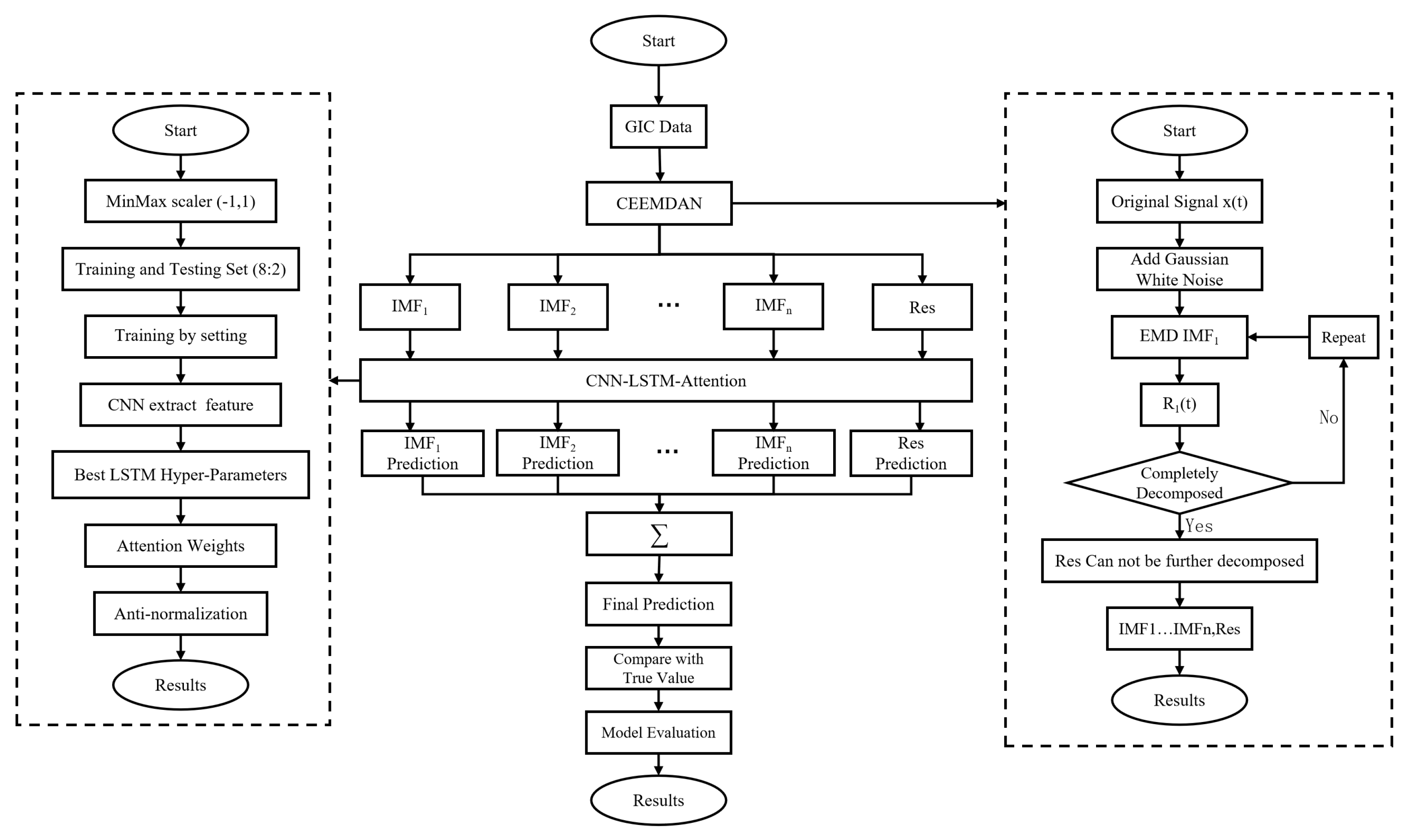
The primary modeling approach presented in this paper is outlined as follows: Initially, the GIC data are decomposed adaptively into a series of Intrinsic Mode Functions (IMFs) and residuals (R) using the Complete Ensemble Empirical Mode Decomposition with Adaptive Noise (CEEMDAN). Subsequently, a CNN is employed to efficiently extract features from these IMFs, which are then fed into a LSTM network for training. This process can deeply derive the information from various time scales within the time series signal. An attention mechanism is subsequently applied to assign weights to salient features, thereby enhancing model learning efficiency. Ultimately, the predicted sequences from all IMFs and R are aggregated to derive the final prediction outcome. The model’s performance is subsequently assessed using several standard quantitative metrics. The subsequent sections will provide a concise overview of the principal analysis methodologies.

2.1. CEEMDAN

EMD represents an adaptive time-frequency analysis technique, fundamentally facilitating the stationary processing of signals [19]. Zhaohua Wu and Huang proposed the Ensemble Empirical Mode Decomposition (EEMD) [20], which improved significantly the mode mixing issue in EMD by incorporating white noise into the signal to be decomposed and subsequently averaging the resultant decompositions. Further enhancing these methods, TORRES et al. [21] developed the CEEMDAN algorithm, it not only mitigated the mode mixing prevalent in EMD but also effectively eliminates the residual Gaussian white noise associated with the EEMD process.

The processing procedure of CEEMDAN is as follows:

Add Gaussian white noise to the original signal:

$x_{i} (t) = x (t) + ω_{0} ε_{i} (t) i \in 1, \dots, N$

(1)

In the formula, $x (t)$ is the original signal, $ε_{i} (t)$ is the adaptive Gaussian white noise added in the $i^{t h}$ processing, $ω_{0}$ is the signal-to-noise ratio between the noise and the original signal, $x_{i} (t)$ is the new signal generated after adding white noise for the $i^{t h}$ time, and N is the number of integrations.
After decomposition of $x_{i} (t)$ , multiple intrinsic mode sequences and residuals are obtained:

$C_{i} (t) = \frac{1}{N} \sum_{i = 1}^{N} C_{1}^{i} (t)$

(2)

$R_{1} (t) = x (t) - C_{1} (t)$

(3)

In the formula, N is the number of components, $C_{1} (t)$ is the first IMF component obtained by CEEMDAN decomposition, $C_{i} (t)$ is the $i^{t h}$ intrinsic mode obtained after decomposition, $R_{1} (t)$ is the residual obtained after the first decomposition.
Add adaptive Gaussian white noise to $R_{1} (t)$ to obtain a new signal. Repeat the above steps to obtain other intrinsic modes and residuals:

$C_{k} (t) = \frac{1}{N} \sum_{i = 1}^{N} E_{1} [r_{k - 1} + ω_{k - 1} E_{k - 1} ε_{i} (t)]$

(4)

$R_{k} (t) = x (t) - \frac{1}{N} - \sum_{i = 1}^{k} C_{k} (t)$

(5)

In the formula, $C_{k} (t)$ is the th component obtained by CEEMDAN decomposition, $R_{k} (t)$ is the residual signal at the $k^{t h}$ stage, $E_{k - 1}$ is the ${(k - 1)}^{t h}$ component after decomposition, $ω_{k - 1} E_{k - 1} E_{k - 1}$ is the signal-to-noise ratio added in the ${(k - 1)}^{t h}$ stage, k is the total number of modes.
Repeat the above steps until R cannot be decomposed anymore. The decomposition result of the original signal $x (t)$ by CEEMDAN can be expressed as:

$x (t) = \sum_{i = 1}^{k} C_{k}^{(} t) + R_{k} (t)$

(6)

2.2. CNN

CNNs are among the most prevalent models in deep learning [22]. They comprise principal components such as convolutional layers, pooling layers, and fully connected layers. CNNs utilize convolutional and pooling layers to extract diverse feature vectors from input data using convolution kernels. The "ReLU" activation function is then applied for dimensionality reduction by diminishing the influence of less significant features. As a specialized form of deep feedforward network, CNNs are extensively employed for processing time series, images, and audio. Two-dimensional CNNs (Conv2D) are particularly prevalent in image recognition and processing, while one-dimensional CNNs (Conv1D) are more suitable for time series prediction tasks. Consequently, this study employs Conv1D to extract features from data, which are subsequently integrated with LSTM for training. The local receptive fields and weight sharing characteristics of CNNs diminish the complexity of the input matrices and the computational load of the model, thereby enhancing the training efficiency and predictive accuracy of the LSTM.

The structure of the CNN neural network is shown in Figure 1. The lower boxes in the figure from left to right represent: input layer, convolution kernel, convolution layer, pooling layer, fully connected layer, and output layer. The calculation method of convolution is as follows:

C_{i} = f_{c} (y_{i} * W_{i} + B_{c})

(7)

In the formula,

C_{i}

is the output result of convolution,

f_{c}

is the Relu activation function of this convolution layer;

y_{i}

is the input of the

i^{t h}

convolution layer;

W_{i}

is the weight of this convolution kernel connected to the

i^{t h}

feature;

B_{c}

is the bias matrix of this convolution layer.

2.3. LSTM

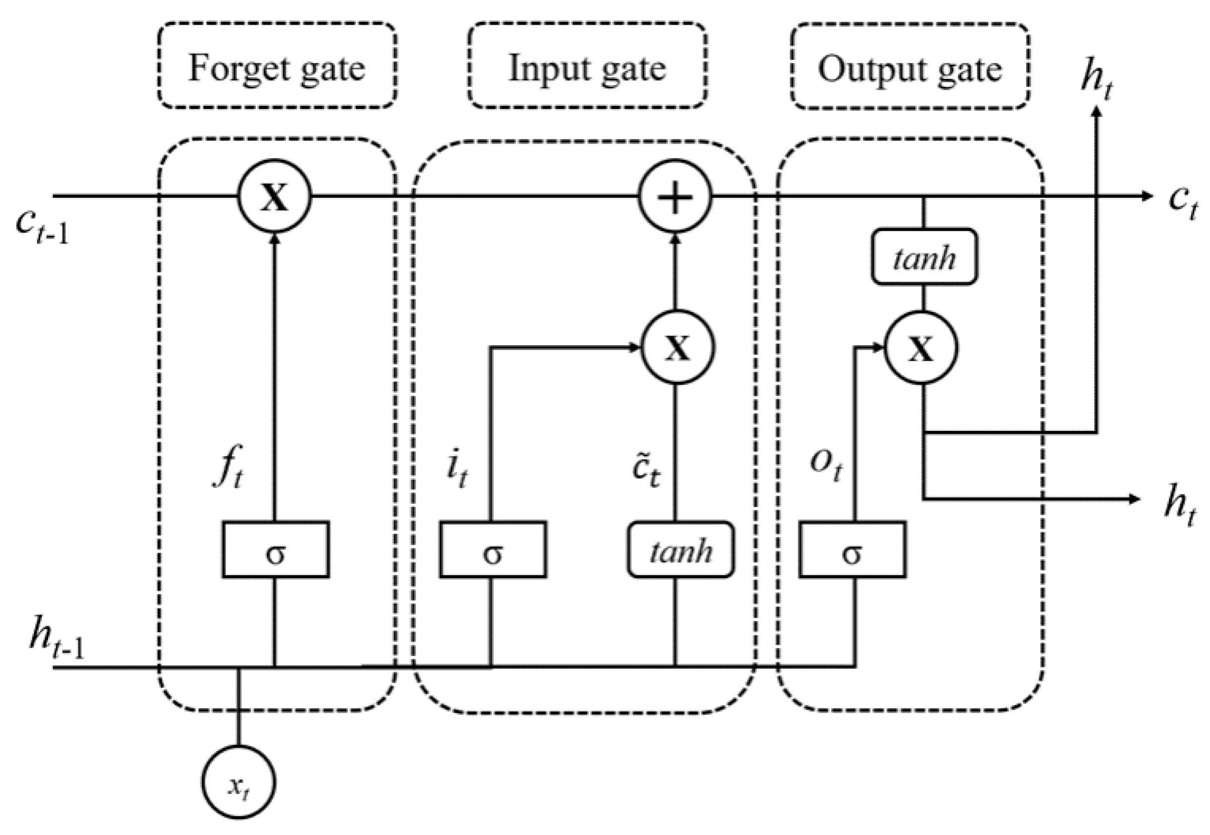
The LSTM network is a variant of the RNN engineered to address the challenges of gradient explosion and vanishing gradients that commonly afflict RNNs [18]. LSTM incorporates a "memory cell" along with three regulatory gate mechanisms—an input gate, a forget gate, and an output gate—which collectively govern the flow of information within the network. This architecture enhances the prediction of time series data, making LSTM extensively utilized in such predictive tasks. Specifically, the input gate ascertains whether new input information should be integrated into the memory cell; the forget gate evaluates which information should be erased from the memory cell; and the output gate manages the transfer of information from the memory cell to the subsequent layer or the network’s output.

The structure of the LSTM neural network is shown in Figure 2. Use

x_{t}

to represent the GIC input data.

i_{t}

represents the input data in t.

f_{c}

is the forgotten data in t.

o_{t}

is the output data in t.

h_{t - 1}

and

c_{t - 1}

are the hidden state and cell state in

t - 1

, where nonlinearity is added in the form of

s i g m o i d

and activation functions[14].

Forgetting Gate Function:

f_{t} = σ (W_{f} \cdot [h_{t - 1}, X_{t}] + b_{f})

(8)

Input gate function:

i_{t} = σ (W_{i} \cdot [h_{t - 1}, X_{t}] + b_{i})

(9)

{\bar{c}}_{t} = t a n h (W_{c} \cdot [h_{t - 1}, X_{t}] + b_{c})

(10)

Unit Status:

C_{t} = f_{i} * c_{t - 1} + i_{t} * {\bar{c}}_{t}

(11)

Output gate function:

o_{i} = σ (W_{0} \cdot [h_{t - 1}, X_{t}] + b_{0})

(12)

Unit hidden layer output:

h_{t} = o_{t} * t a n h (C_{t})

(13)

Sigmoid Function:

σ (x) = \frac{1}{1 + e^{- x}}

(14)

tanh:

t a n h (x) = \frac{e^{x} - e^{- x}}{e^{x} + e^{- x}}

(15)

In each of the above functions,

W_{f}

W_{i}

W_{c}

and

W_{o}

are the corresponding weight matrices of the forget gate, input gate, memory cell, and output gate respectively.

b_{f}

b_{i}

b_{c}

and

b_{o}

respectively represent the bias terms of the forget gate, input gate, memory cell, and output gate. * represents the Hadamard product of matrices.

2.4. Attention Mechanism

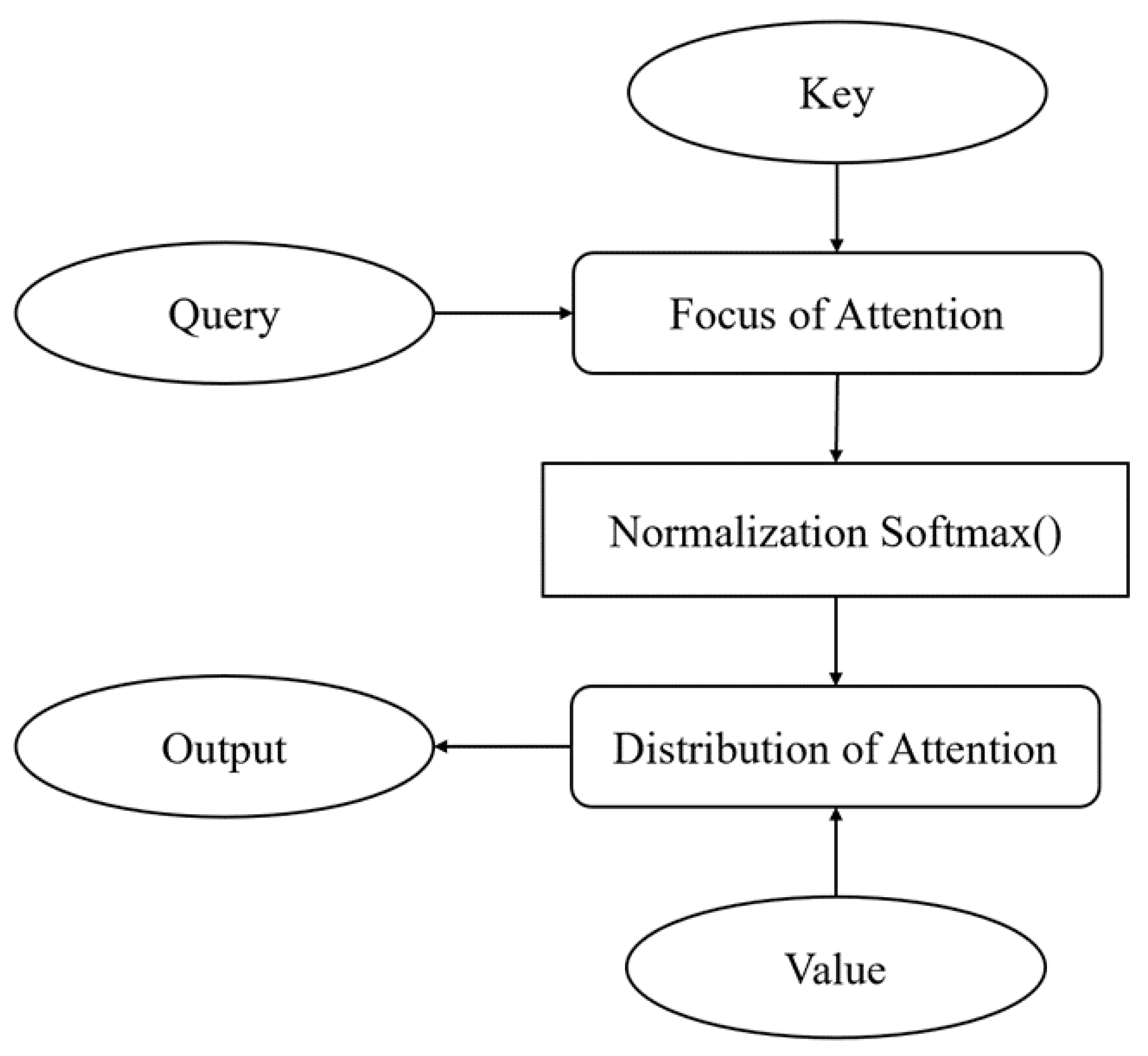
The attention mechanism emulates human attentive processes, enabling models to discern salient from less relevant components within data by assigning weight coefficients. This mechanism leverages the intrinsic information contained within data features for attentional interactions, facilitating the allocation of limited resources to pertinent input segments while disregarding irrelevant interference. Consequently, it enhances the operational efficiency and predictive accuracy of machine learning models [23].

The attention mechanism structure is shown in Figure 3. Firstly, the correlation between the query vector Q (Query) and the key vector K (Key) matrix is calculated through the attention convergence function F. The correlation is normalized to -1 1 by the Softmax function. Finally, the attention score is multiplied by the V (Value) matrix to redistribute the values in the V matrix [23].

Q = X \cdot W_{q}

(16)

K = Y \cdot W_{k}

(17)

V = Z \cdot W_{v}

(18)

W_{q}

W_{k}

W_{v}

is the corresponding weight parameter

A t t e n t i o n (Q, K, V) = S o f t m a x (\frac{Q \cdot K^{T}}{\sqrt{d_{k}}})

(19)

In the formula,

d_{k}

is the dimension of K and has a scaling effect on the value after the dot product of Q and K.

3. Training and Testing

3.1. Procedure

This paper proposes a short-term GIC prediction method based on the CEEMDAN-CNN-LSTM-Attention network. The model structure is shown in Figure 4. Specifically, it includes the following steps:

Decompose the GIC data by CEEMDAN to obtain the intrinsic modes $I M F_{1}$ , $I M F_{2}$ ... $I M F_{n}$ and the R;
The intrinsic modes and residual are respectively normalized by MinMax to the interval (-1, 1), and the data sets are divided according to 8:2 for both;
The training set is input into the CNN to further extract features, and then the training set after feature extraction enters the LSTM layer for training, and then enters the Attention layer to adjust the training weights. During the training process, different hyperparameters are input, and the grid search method (Grid SeaschCV) is used to find the best hyperparameters;
Obtain the final inverse-normalized training result with the best hyperparameters. Then accumulate the prediction results of different intrinsic modes and compare them with the observed data, and conduct a comprehensive evaluation of the prediction model.

The CPU used for training the model is 12th Gen Intel(R) Core(TM) i5-12500H at 2.50 GHz, and the RAM is 16.0 GB. The neural network model constructed using python3.8.3 in this paper involves seven libraries: numpy 1.23.4, pandas 1.5.3, matplotlib 3.7.1, sklearn 1.1.3, tensorflow-cpu 2.4.1, and keras 2.4.3. Among them, numpy and pandas are used for data preprocessing. The plt function in matplotlib is used to draw images. The MinMaxScaler function in sklearn is used for normalization. The tensorflow and keras libraries are used to build CNN, LSTM, and Attention models.

3.2. Evaluation

In order to facilitate the comparison of the prediction performance of each group of models, this paper uses the coefficient of determination (

R^{2}

), root mean squared error (RMSE), and mean absolute error (MAE) to evaluate the algorithm model[17]. Specific as follows:

R^{2} = 1 - \frac{R M S E}{V a r}

(20)

R M S E = \sqrt{\frac{1}{n} \sum_{k = 1}^{n} {(t_{k} - y_{k})}^{2}}

(21)

M A E = \frac{1}{n} \sum_{k = 1}^{n} |t_{k} - y_{k}|

(22)

In equations (21) and (22), n represents the number of predicted values participating,

y_{k}

represents the predicted value of the model,

t_{k}

represents the true value of the site, and

V a r

represents the variance of the predicted value. Among them,

R^{2}

represents the fitting degree of the model. The closer the value of

R^{2}

is to 1, the better the model prediction effect; the closer the values of the two indicators RMSE and MAE are to 0, the better the model prediction effect and the smaller the error.

4. Results

4.1. Data

The GIC data employed in this study were obtained from the direct current (DC) monitoring at the neutral point of a transformer within the Lingao Nuclear Power Station in Guangdong. The station is situated at a geographic coordinate of 22.6° N latitude and 114.6° E longitude. The data collection spanned two periods: from 10:30 UT on November 7, 2004 to 12:30 UT on November 8, 2004, and from 18:30 UT on November 9, 2004 to 22:30 UT on November 10, 2004. To aviod redundancy, the text presents results solely for the interval between the 7th and 8th. Data and outcomes for the 9th to the 10th are provided as supplementary material. The sampling interval for the original signal was 1 second. The corresponding relative variation geomagnetic field data were derived from the X, Y, and Z components recorded at the Zhaoqing Geomagnetic Station in Guangdong, which is located at 23.1° N latitude and 112.3° E longitude.The geomagnetic disturbance index SYM-H is taken from OMNI in the Coordinated Data Analysis Web(https://cdaweb.gsfc.nasa.gov/index.html).

4.2. Events

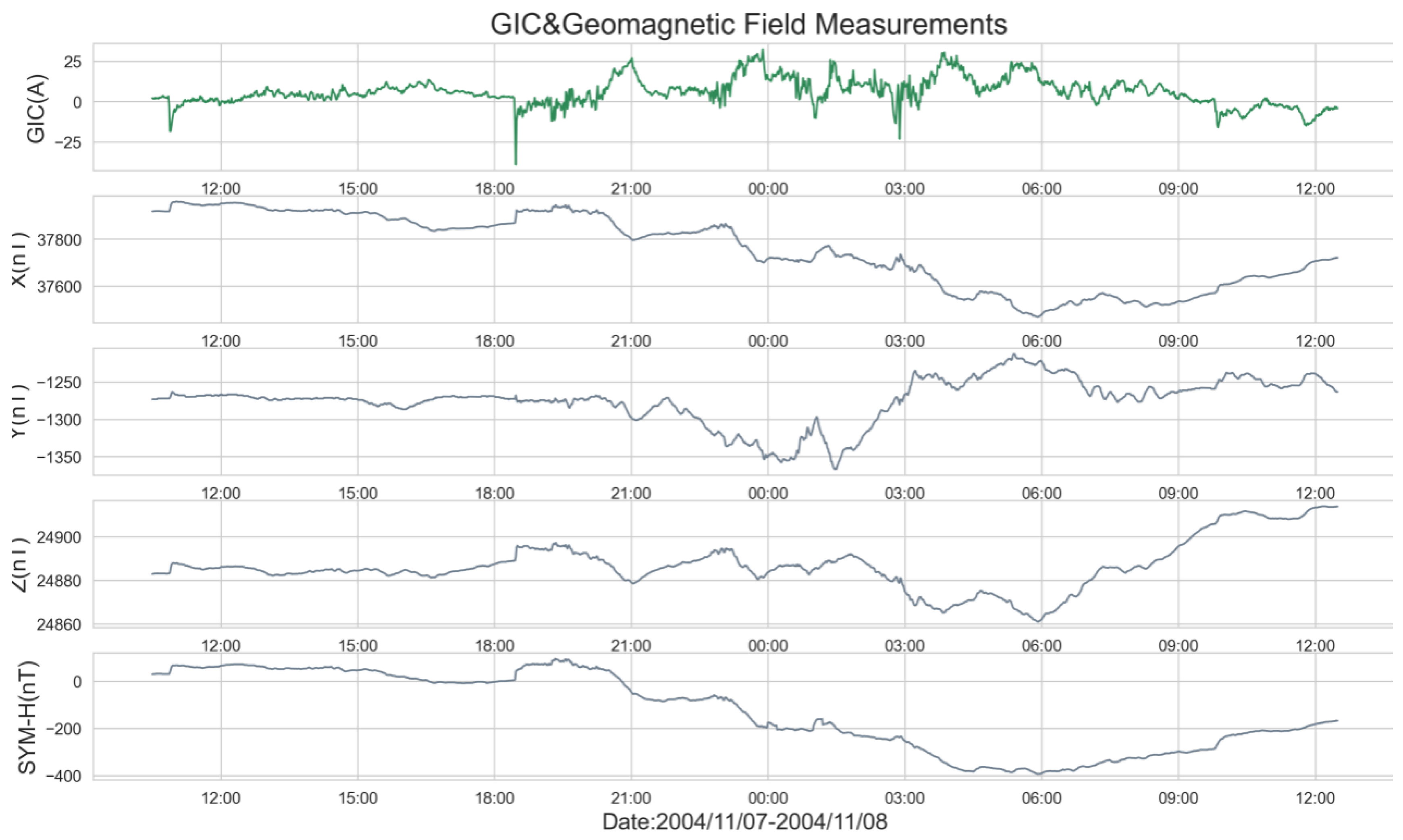
The waveform diagrams of the original GIC signals, the three components of the geomagnetic field, and the geomagnetic disturbance index are depicted in Figure 5. The time span covers from 10:30 UT on November 7, 2004, to 12:30 UT on November 8, 2004, totaling 26 hours. The GIC and the three geomagnetic field components are sampled at a rate of 1 second, whereas the geomagnetic disturbance index is sampled at a rate of 1 minute. Consequently, the GIC and geomagnetic field components’ sampling rate is downscaled to 1 minute using a sliding average method, resulting in a dataset comprising 1560 entries.

The green solid line depicted in the figure represents the GIC observation data from the Lingao Nuclear Power Station. The descending gray solid lines represent the north (X), east (Y), and vertical (Z) components of the geomagnetic field as observed by the Zhaoqing Geomagnetic Station, along with the geomagnetic disturbance index (SYM-H). The data evolution curve illustrates that the GIC observation data exhibit characteristics of instability and substantial fluctuations. Throughout the geomagnetic storm, all three components of the geomagnetic field—X, Y, and Z—demonstrate notable instantaneous disturbance traits. The amplitude variation of the X component during the principal phase of the storm is approximately -500 nT. The GIC intensity peaks at approximately -40 A at 18:28 on November 7, coinciding with a SYM-H value as low as -394 nT.

The division of GIC data into training and testing sets is illustrated in Figure 6. The portion represented by the green solid line in Figure 6 serves as the GIC training set, comprising a total of 74,880 data samples. Inclusion of the GIC peak value within the training set significantly enhances the model’s predictive performance. Conversely, the red solid line denotes the prediction set, which consists of 18,720 data samples.

4.3. CEEMDAN of GIC Sequences

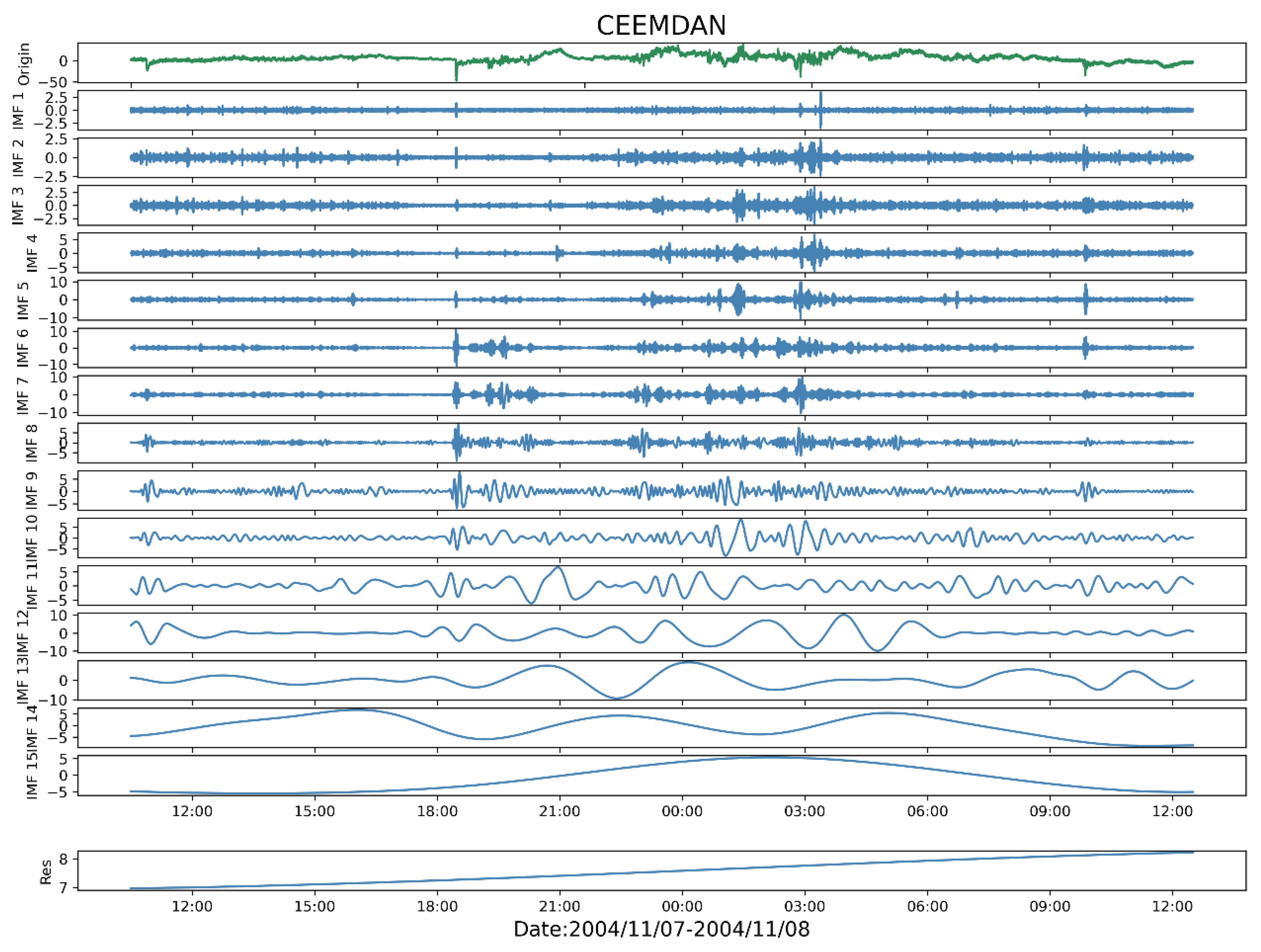
The GIC signal diagram obtained by decomposing the GIC prediction analysis sample by CEEMDAN is shown in Figure 7. The green solid line is the observed time series of GIC, and the blue solid line is the intrinsic modes

I M F_{s}

and R obtained by decomposing by the CEEMDAN method. Through the adaptive CEEMDAN process, the GIC time series is decomposed into 15 intrinsic modes and residuals.

4.4. IMFs Prediction

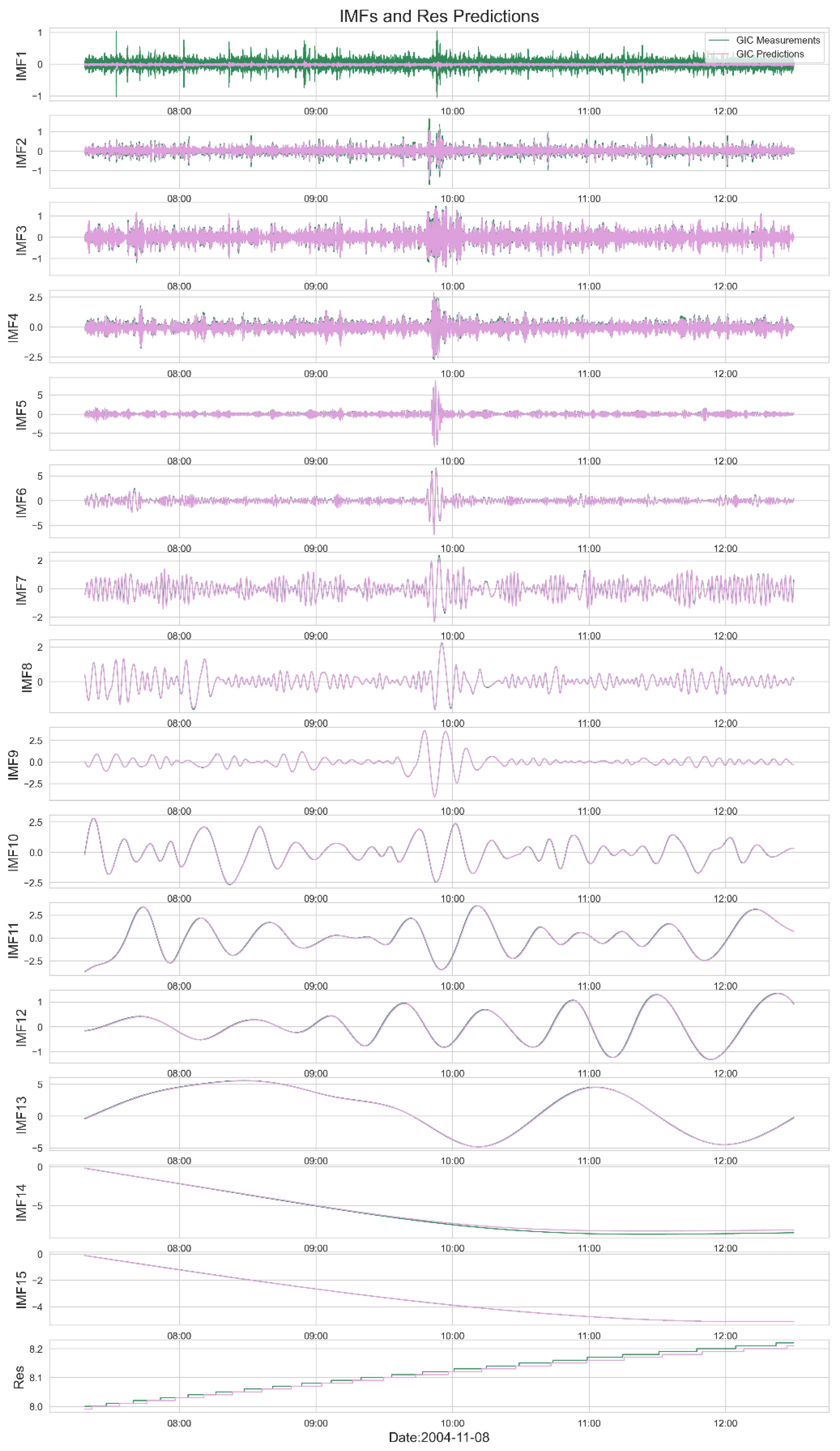
The 15 intrinsic modes IMF and residual R obtained by CEEMDAN decomposition are respectively input into the CNN-LSTM-Attention model for prediction. The results are shown in Figure 8.

The figure presents the prediction outcomes of the intrinsic modes (IMF1 to IMF15) and residuals (R) derived from the CEEMDAN decomposition of the GIC test sample, arranged from top to bottom. The green solid line represents the original observed values, whereas the pink solid line signifies the predicted values. As depicted in Figure 8, the prediction accuracy for the IMF1 component is notably deficient. This analysis suggests that the white noise introduced by the CEEMDAN method impedes the machine learning model’s ability to make precise predictions, which is identified as the primary source of error in the composite model’s GIC predictions within this study.

4.5. GIC Prediction

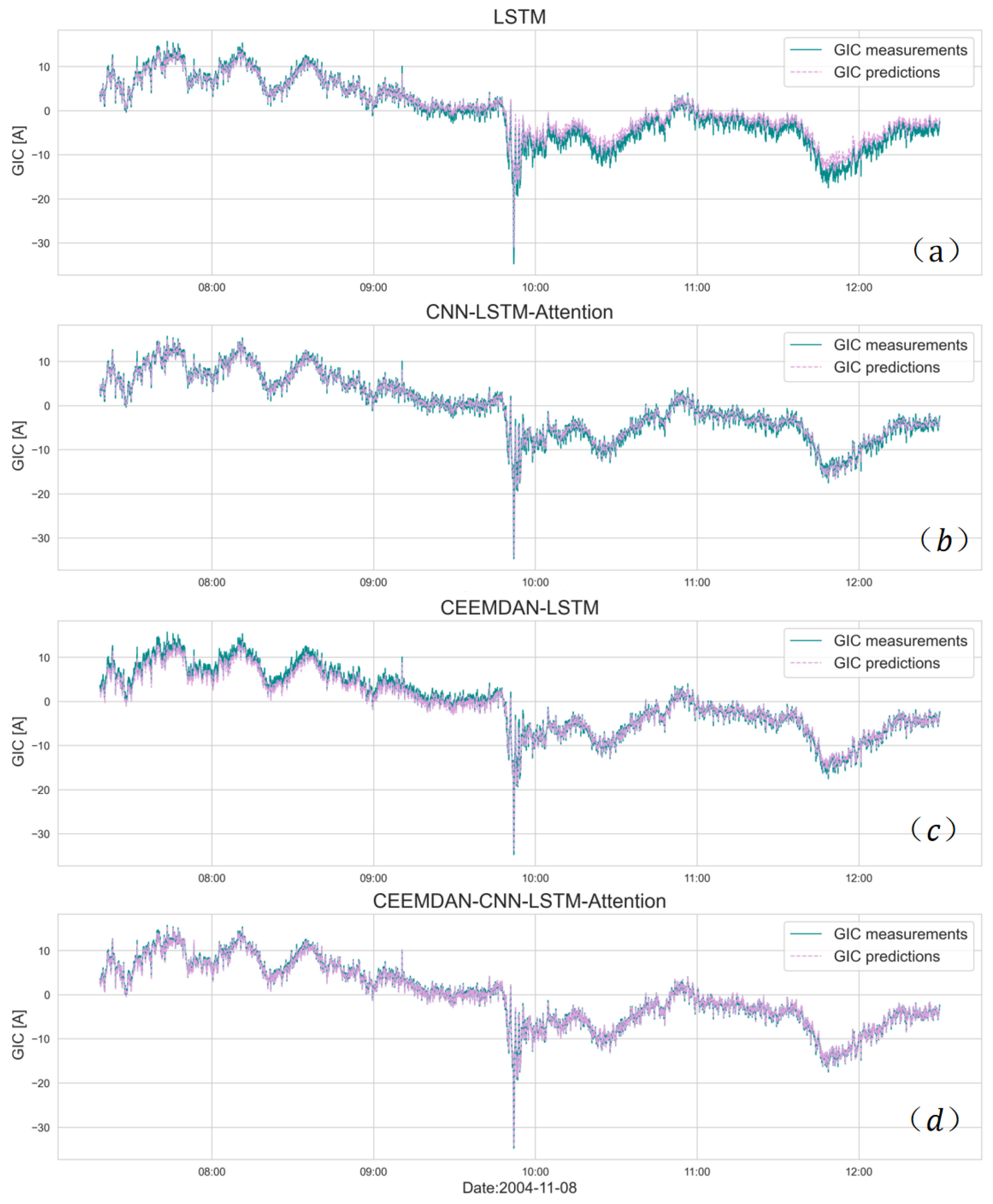
Figure 9 illustrates the prediction results derived from various neural network combination methods over the entire time span from 07:18 to 12:30 on November 8, 2004. Arranged from top to bottom, the panels (a), (b), (c), and (d) represent the predictive performance of the LSTM model, the CNN-LSTM-Attention model, the CEEMDAN-LSTM model, and the CEEMDAN-CNN-LSTM-Attention model, respectively. The green solid line within the figure denotes the GIC measurement values, while the pink dotted line indicates the GIC prediction values. An assessment of the overall prediction efficacy reveals that the LSTM model overestimates the actual values by approximately two hours post-storm; however, the integration of CNN and Attention mechanisms enhances the predictive accuracy. Although the CEEMDAN-LSTM model exhibits deficiencies in forecasting two hours prior to the storm, the CEEMDAN-CNN-LSTM-Attention model demonstrates significant improvements in overall predictive performance.

The comparative evaluation metrics for various combined models are presented in Table 1. The LSTM model exhibits the lowest coefficient of determination (R²) for GIC prediction, with the highest root mean square error (RMSE) and mean absolute error (MAE), suggesting that the predictive performance of this standalone model is somewhat inadequate relative to hybrid models. The CEEMDAN-CNN-LSTM-Attention model achieves an R² of 99.4%, with an RMSE of merely 0.54 and an MAE as low as 0.41. When contrasted with the LSTM, CNN-LSTM-Attention, and CEEMDAN-LSTM models, the CEEMDAN-CNN-LSTM-Attention model has enhanced the R² by 3.1%, 1.4%, and 1.3%, respectively. It has also decreased the RMSE by 0.82 A, 0.47 A, and 0.45 A, respectively, and the MAE by 0.63 A, 0.30 A, and 0.37 A, respectively. Overall, while the LSTM model’s predictive efficacy is adequate for most scenarios, employing the CEEMDAN-CNN-LSTM-Attention model yields more precise outcomes.

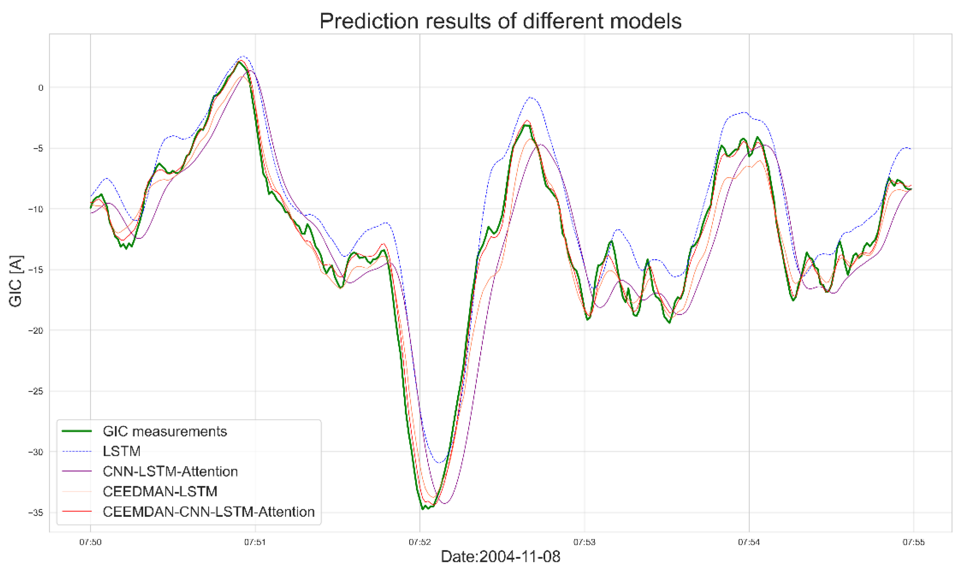
Figure 10 displays the GIC prediction results during the storm period, utilizing various neural network combination methods between 07:50 and 07:55 on November 8, 2004. Within the figure, the green bold solid line represents the measured GIC values, the blue dotted line signifies the GIC predictions from the LSTM model, the purple solid line indicates those from the CNN-LSTM-Attention model, the orange solid line denotes the predictions from the CEEMDAN-LSTM model, and the red solid line represents the CEEMDAN-CNN-LSTM-Attention model’s predictions.

As can be seen from Figure 10:

The GIC value predicted by the LSTM model is larger than the real value. After adding CNN and Attention, the predicted value of the CNN-LSTM-Attention model is closer to the real value.
The GIC response speed of the LSTM model and the CNN-LSTM-Attention model has a delay of about 3 seconds. This delay phenomenon has also been observed in other studies using LSTM for prediction[24]. One possible reason: The LSTM model algorithm uses fixed time window samples for training and learning. In order to minimize the error, using the value at t as the predicted value at $t + 1$ not only requires no additional operations but also has a small error, resulting in a delay in the final prediction.
The CEEMDAN-LSTM model and the CEEMDAN-CNN-LSTM-Attention model can reduce the time delay of the GIC response during geomagnetic storms by about 3 seconds by decomposing and predicting GIC data and then accumulating.
In terms of overall prediction performance, the CNN-LSTM-Attention model and the CEEMDAN-LSTM model are close in prediction performance. However, in the response during geomagnetic storms, the CEEMDAN-LSTM model is significantly better than the CNN-LSTM-Attention model. This shows that adding the CEEMDAN method can effectively reduce prediction delay and thus improve prediction performance.

The evaluation indexes of GIC during geomagnetic storms of the four models are shown in Table 1. It can be seen that:

For the LSTM model, R2 is the lowest at 0.830, and RMSE and MAE are the highest, at 3.00A and 2.45A respectively.
The CNN-LSTM-Attention model adds CNN and Attention to improve the prediction effect. R2, RMSE and MAE are 0.850, 2.82A and 2.22A respectively.
The CEEMDAN-LSTM model after adding the CEEMDAN method has a reduced degree of delay. And since it is decomposed into IMFn and R, which reduces the difficulty of machine learning, the prediction effect is greatly improved. R2, RMSE and MAE are 0.949, 1.63A and 1.26A respectively.
The CEEMDAN-CNN-LSTM-Attention model has the highest R2 at 0.992, and the lowest RMSE and MAE at 0.64A and 0.50A respectively, verifying that the CEEMDAN-CNN-LSTM-Attention model proposed in this paper shows good prediction performance when predicting GIC during geomagnetic storms.

5. Discussion

This study utilizes GIC data collected during the November 2004 geomagnetic storm. Employing a suite of technical methodologies, including CEEMDAN, CNN, LSTM, and Attention mechanisms, we conducted a comprehensive analysis and testing of the predictive performance of hybrid neural network models in comparison to individual neural networks. This approach offers a more robust technical framework for the development of GIC early warning and predictive systems. Leveraging local power grid observation data, the paper presents a thorough comparative analysis of various combinations of these technical methods. This analysis assesses the accuracy and error of model predictions against actual measurements. The findings of the research are as follows:

This paper addresses the inherent instability and nonlinearity of GIC data observed during geomagnetic storms by employing the CEEMDAN method for data preprocessing. This approach decomposes the GIC data into intrinsic mode signals across multiple time scales, thereby enhancing data stability. The integration of CEEMDAN with LSTM yields a significant enhancement in predictive accuracy compared to the use of LSTM alone. Moreover, the CEEMDAN-LSTM model effectively mitigates the time delay issues associated with responses to geomagnetic storms, leading to improved overall prediction performance.
The predictive performance of the CNN-LSTM-Attention model, which incorporates both CNN and Attention mechanisms, surpasses that of the LSTM model alone. This enhancement suggests that the CNN effectively captures instantaneous features from the data, while the Attention mechanism refines the model’s accuracy by dynamically adjusting the weights assigned to different features.

Based on the above results, the limitations existing in this study are explained and discussed as follows:

Due to the general scarcity of continuous GIC monitoring in actual power grid research, this paper is constrained to a limited number of storm samples for training and testing the predictive model. Consequently, the hybrid model, trained on this modest historical dataset, currently lacks the practical predictive capability for GIC. This limitation also extends to its generalizability and universal applicability to a certain extent.
The hybrid neural network prediction model presented in this study employs GIC data for single-step forecasting. Given that CEEMDAN is capable of executing only single-sequence decomposition per iteration, the temporal efficiency of sequentially decomposing multiple input parameters merits consideration when developing a multi-parameter GIC prediction model. Concurrently, the intrinsic modes derived from CEEMDAN decomposition are collectively processed using a CNN-LSTM-Attention architecture, which functions as a multi-input and multi-output system. Naturally, variations exist in the number of intrinsic modes fed into the modeling process, and the resulting trained models exhibit minor discrepancies.

Despite the numerous limitations inherent in the local short-term GIC prediction approach outlined in this paper, these constraints do not preclude a discussion on the viability of deep learning within the realm of GIC research from a technical integration standpoint. With the advent of more advanced conditions, such as the acquisition of a sufficient dataset of power grid GIC during geomagnetic storms and the development of a comprehensive sample repository, it becomes feasible to integrate local solar wind parameters and geomagnetic field data. This integration aims to develop a dynamic, composite neural network model designed for practical application in GIC forecasting.

Author Contributions

Investigation, Wenhao Chen. Data curation, Haiyang Jiang. Funding acquisition, Jin Liu. All authors have read and agreed to the published version of the manuscript.

Funding

This work was supported by the National Nature Science Foundation of China (grants No. 41664008 and 42464010)

Data Availability Statement

The geomagnetic disturbance index SYM-H is taken from OMNI in the Coordinated Data Analysis Web. The website is as follows:https://cdaweb.gsfc.nasa.gov/index.html.

Conflicts of Interest

The authors declare that they have no known competing financial interests or personal relationships that could have appeared to influence the work reported in this paper.

References

F. R ,N. A ,N. L , et al. Investigating the Magnetic Structure of Interplanetary Coronal Mass Ejections Using Simultaneous Multispacecraft In Situ Measurements. The Astrophysical Journal 2023, 957, 1. [Google Scholar] [CrossRef]
Rajkumar, H. Intense, Long-Duration Geomagnetically Induced Currents (GICs) Caused by Intense Substorm Clusters. Space Weather 2022, 20, 3. [Google Scholar] [CrossRef]
XinW ,LiuC ,WangG , et al. Vibration characteristics of a single-phase four-column auto-transformer core excited by geomagnetically induced currents. IET Electric Power Applications 2024, 18, 766–778. [Google Scholar] [CrossRef]
David O ,Pitambar J. Power system harmonic analysis with real geomagnetically induced current from the 2003 halloween storm. Scientific African 2024, 22. [Google Scholar] [CrossRef]
Zan-ming C ,Chun-ming L ,An-qi L , et al. Modeling Calculation and Influencing Factors of Geomagnetically Induced Current in Sanhua Power Grid. Journal of Physics: Conference Series 2023, 2564, 1. [Google Scholar] [CrossRef]
Liu C ,Liu L ,Pirjola R , et al. Calculation of geomagnetically induced currents in mid- to low-latitude power grids based on the plane wave method: A preliminary case study. Space Weather 2024, 7, 4. [Google Scholar] [CrossRef]
Pirjola, R. and Viljanen, A. Complex image method for calculating electric and magnetic fields produced by an auroral electrojet of a finite length. Annales Geophysicae 1998, 16, 1434–1444. [Google Scholar] [CrossRef]
Boteler, D.H. and Pirjola, R.J. The complex-image method for calculating the magnetic and electric fields at the surface of the Earth by the auroral electrojet. Geophysical JournalInternational 1998, 132, 31–40. [Google Scholar] [CrossRef]
A. V ,A. P ,O. A , et al. Fast computation of the geoelectric field using the method of elementary current systems and planar Earth models. Annales Geophysicae 2024, 22, 101–113. [Google Scholar] [CrossRef]
Ngwira M C ,McKinnell L ,Cilliers J P , et al. Limitations of the modeling of geomagnetically induced currents in the South African power network. Space Weather 2009, 7, 10. [Google Scholar] [CrossRef]
Wintoft, P. , er al. Study of the solar wind coupling to the time difference horizontal geomagnetic field. Annales Geophysicae 2005, 23, 1949–1957. [Google Scholar] [CrossRef]
V. P ,O. K ,M. H , et al. Is the Global MHD Modeling of the Magnetosphere Adequate for GIC Prediction: the May 27–28, 2017 Storm. Cosmic Research 2023, 61, 120–132. [Google Scholar] [CrossRef]
Zhang J J ,Yu Q Y ,Wang C , et al. Measurements and Simulations of the Geomagnetically Induced Currents in Low-Latitude Power Networks During Geomagnetic Storms. Space Weather 2020, 18, 8. [Google Scholar] [CrossRef]
Tan, Y. , Hu, Q., Wang, Z., Zhong, Q. Geomagnetic index Kp forecasting with LSTM. IET Electric Power Applications 2018, 16, 406–416. [Google Scholar] [CrossRef]
Camporeale S C G A M. Multiple-Hour-Ahead Forecast of the Dst Index Using a Combination of Long Short-Term Memory Neural Network and Gaussian Process. Space Weather 2018, 18, 1882–1896. [Google Scholar] [CrossRef]
Zhang, H. , Xu, H. R., Peng, G. S., Qian, Y. D., Zhang, X. X., Yang, G. L., et al. A prediction model of relativistic electrons at geostationary orbit using the EMD-LSTM network and geomagnetic indices. Space Weather 2022, 20, 1029. [Google Scholar] [CrossRef]
Cid M C A. Deep Neural Networks With Convolutional and LSTM Layers for SYM-H and ASY-H Forecasting. Space Weather 2021, 19, 6. [Google Scholar] [CrossRef]
Bailey, R. L. , Leonhardt, R., Möstl, C., Beggan, C., Reiss, M. A., Bhaskar, A., Weiss, A. J. Forecasting GICs and geoelectric fields from solar wind data using LSTMs: Application in Austria. Space Weather 2022, 20. [Google Scholar] [CrossRef]
Huang, N.E. , Shen, Z., Long, S.R., et al. The empirical mode decomposition and the Hilbert spectrum for nonlinear and non-stationary time series analysis. Proceedings of the Royal Society of London Series A: mathematical, physical and engineering sciences 1998, 454, 903–995. [Google Scholar] [CrossRef]
Wu, Z. , Huang, N.E. Ensemble empirical mode decomposition: a noise-assisted data analysis method. Advances in adaptive data analysis 2009, 1, 1–41. [Google Scholar] [CrossRef]
Torres, M.E. , Colominas, M.A., Schlotthauer, G., et al. A complete ensemble empirical mode decomposition with adaptive noise. IEEE, 2011. [Google Scholar] [CrossRef]
Rio F ,Matthew B H ,Maria C , et al. Facial expression recognition using bidirectional LSTM-CNN. Procedia Computer Science 2023, 47, 21639. [Google Scholar]
Yuan G ,Chengkuan F ,Yingjun R. A novel model for the prediction of long-term building energy demand: LSTM with Attention layer. IOP Conference Series: Earth and Environmental Science 2019, 18294012033, 012033. [Google Scholar] [CrossRef]
Jianxian C ,Xun D ,Li H , et al. An Air Quality Prediction Model Based on a Noise Reduction Self-Coding Deep Network. Mathematical Problems in Engineering 2020, 2020. [Google Scholar] [CrossRef]

Figure 1. This is structure of convolutional neural network.

Figure 2. Structure of Long-Short-Term Memory Neural Network.

Figure 3. Structure of Long-Short-Term Memory Neural Network.

Figure 4. Structure of Long-Short-Term Memory Neural Network.

Figure 5. Curve of near-Earth space data over time during the magnetic storm period from November 7 to 8, 2004.

Figure 6. Partition of GIC training and testing sets.

Figure 7. GIC decomposition results based on CEEMDAN.

Figure 8. CEEMDAN decomposition of the predicted values of each IMF component and R component compared with the original data.

Figure 9. GIC prediction results based on different models.

Figure 10. Prediction results of GIC during storms under different models.

Table 1. This is a table caption. Tables should be placed in the main text near to the first time they are cited.

Model	R²	RMSE/A	MAE/A
LSTM	0.963	1.36	1.04
CNN-LSTM-Attention	0.980	1.01	0.71
CEEMDAN-LSTM	0.981	0.99	0.78
CEEMDAN-CNN-LSTM-Attention	0.994	0.54	0.41

Table 2. This is a table caption. Tables should be placed in the main text near to the first time they are cited.

Model	R²	RMSE/A	MAE/A
LSTM	0.830	3.00	2.45
CNN-LSTM-Attention	0.850	2.82	2.22
CEEMDAN-LSTM	0.949	1.63	1.26
CEEMDAN-CNN-LSTM-Attention	0.992	0.64	0.50

Disclaimer/Publisher’s Note: The statements, opinions and data contained in all publications are solely those of the individual author(s) and contributor(s) and not of MDPI and/or the editor(s). MDPI and/or the editor(s) disclaim responsibility for any injury to people or property resulting from any ideas, methods, instructions or products referred to in the content.

© 2024 by the authors. Licensee MDPI, Basel, Switzerland. This article is an open access article distributed under the terms and conditions of the Creative Commons Attribution (CC BY) license (http://creativecommons.org/licenses/by/4.0/).

Copyright: This open access article is published under a Creative Commons CC BY 4.0 license, which permit the free download, distribution, and reuse, provided that the author and preprint are cited in any reuse.

Alerts

MDPI Initiatives

Important Links

Choose an area of interest and we will send you notifications of new preprints at your preferred frequency.

Disclaimer

Preliminary Exploration on Short-Term Prediction of Local Geomagnetically Induced Currents Using Hybrid Neural Networks

Abstract

Keywords:

Subject:

1. Introduction

2. Methodology

2.1. CEEMDAN

2.2. CNN

2.3. LSTM

2.4. Attention Mechanism

3. Training and Testing

3.1. Procedure

3.2. Evaluation

4. Results

4.1. Data

4.2. Events

4.3. CEEMDAN of GIC Sequences

4.4. IMFs Prediction

4.5. GIC Prediction

5. Discussion

Author Contributions

Funding

Data Availability Statement

Conflicts of Interest

References

MDPI Initiatives

Important Links

Subscribe