Submitted:
30 October 2024
Posted:
31 October 2024
You are already at the latest version
Abstract
The instability of double-diffusive convection of an Oldroyd-B fluid in a vertical porous layer caused by temperature and solute concentration differences with the Soret effect is studied using a modified Darcy–Brinkman–Oldroyd model. Under the Oberbeck-Boussinesq approximation, the validity of Squire's theorem is demonstrated, allowing for considering only the two-dimensional linear instability. Based upon perturbation theory, an Orr-Sommerfeld eigenvalue problem is derived and numerically simulated using the Chebyshev collocation method. We examine the effects of the relevant dimensionless parameters on the neutral stability curves. It is discovered that PrD and λ1 have dual effects on the instability, respectively. When PrDc1 < PrD < PrDc2, PrD boosts flow stability. The impact of λ1 on fluid stability is influenced by PrD. Furthermore, Le and η have dual effects on the instability. When η< 0.8, it promotes flow instability. Le enhances the flow in-stability when Le < 0.7 and inhibits the instability when Le > 0.7. In addition, the magnitude of Le influences the role of Sr. There exists a critical value for Le. When Le < Lec2, Sr strengthens the in-stability of the flow, and when Le> Lec2, Sr plays an inhibiting role. Finally, the relaxation pa-rameter λ2 promotes flow stability.
Keywords:
Soret effect
; Oldroyd-B fluid
; Brinkman porous layer
; double-diffusive convection
; instability
1. Introduction
A solid with micropores are called porous media, and these micropores are often interconnected and usually filled with fluid. Porous media encompasses natural substances, such as biological tissues, wood, zeolites, soils, and rocks. Due to its numerous fundamental and industrial applications, double diffusive convection (DDC) in porous media is a phenomenon that occurs in a variety of systems and has attracted a lot of attention in recent decades. These applications include producing high-quality crystals, storing liquid gases, migrating moisture in fiber insulation, transporting contaminants in saturated soils, solidifying molten alloys, and heating lakes and magmas through geothermal processes. Ingham and Pop [1], Nield and Bejan [2], and Vafai [3] have provided comprehensive reviews on this subject.
The stability or instability of fluid flow is a crucial aspect of fluid mechanics in porous media. Research on how buoyancy and shearing forces affect fluid flow stability in a vertical layer of porous media has received significant attention. Gill [4] performed an initial analysis of the stability of natural convection in a vertical porous layer whose boundary is impermeable at different temperatures, using Darcy's law as a framework. He concluded that the system always maintains linear stability. Subsequently, Rees [5] added a temporal derivative of the velocity to the momentum equation and determined that the flow remains linearly stable, which is the same as Gill's conclusion. For porous media with high porosity, Lundgren [6] experimentally confirmed that the extension of Darcy's law by Brinkman is more valid. Shankar et al. [7] investigated the effect of inertial terms on the stability of natural convection in a vertical layer of a porous medium at different temperatures using the Brinkman model. Using the classical linear stability theory, they discovered that instability is caused by the inertia effect.
Viscoelastic fluids naturally exhibit convection when flowing through porous media, which has important implications for reservoir engineering, bioengineering and geophysics. Gözüm and Arpaci [8] initially investigated the stability of natural convection in a vertical layer at various temperatures for a viscoelastic Maxwell fluid. Takashima [9] investigated the same problem with Oldroyd-B fluid. Khuzhayorov et al. [10] proposed a revised Darcy's law for analyzing the viscoelastic properties of saturated porous materials. Using the homogenization method, they discovered a general filtration law that describes the flow of a linear viscoelastic fluid in a porous material. Kim et al. [11] used a modified Darcy model to analyze thermal instability in a horizontal porous layer with saturated Oldroyd-B fluid. The conventional linear stability theory provided the critical conditions for the initiation of convective motion. Using a modified Darcy-Brinkman-Oldroyd model, Zhang et al. [12] investigated the convection of saturated Oldroyd-B fluid in a horizontal porous layer heated from below. They calculated the critical number of stationary and oscillating convection. Sun et al. [13] studied the lower horizontal plate that was heated in a time-periodic pattern. The system changed from a steady convection to a periodic or chaotic state. Barletta and Alves [14] investigated the Gill stability problem for power-law fluids and discovered that Gill's findings are also applicable to the power-law fluid. The Gill problem for Oldroyd-B fluid was addressed by Shankar and Shivakumara [15]. In contrast to the results for Newtonian and power-law fluids, the flow of Oldroyd-B fluid is unstable.
Besides, they [16] considered the situation of local thermal non-equilibrium (LTNE) and instability that existed as well. Then, Shanker and Shivakumara [17] considered the case of a porous layer containing an internal heat source. He established that internal heating and relaxation parameters contribute to system instability. Newtonian fluids flow steady, while Oldroyd-B fluids flow unstable. For double-diffusive convection instead of thermal convection, Wang and Tan [18] used a modified Darcy model to study the stability of Maxwell fluids in porous media with two parallel planes.
Malashetty and Biradar [19] investigated the cross-diffusion effect on DDC. They conducted linear and weakly nonlinear stability analyses using a modified Darcy model with a time derivative term as the momentum equation and found the critical Rayleigh number. Malashetty et al. [20,21] then studied the stability of the Oldroyd-B fluid and the formation of DDC saturated isotropic and anisotropic horizontal porous layers, respectively. As a result, the thermal anisotropy parameter has a dual role in the stability of the flow. Kumar and Bhadauria [22] explored the situation of LTNE, adding a time derivative term to the momentum equation. They discovered that when the interphase heat transfer coefficient was big or small, the system behaved similarly to the local thermal equilibrium (LTE) model. Subsequently, Malashetty et al. [23] investigated the situation of an anisotropic rotating porous layer with LTE and found that the thermal anisotropy parameter has the opposite effect on the onset of convection compared with the no-rotation condition. The onset of DDC in a horizontal porous layer was recently studied by Swamy et al. [24] based on the Darcy-Brinkman-Oldroyd model.
Due to numerous applications in geothermal systems, energy storage devices, thermal insulation, drying technologies, catalytic reactors, and nuclear waste repositories, theoretical and experimental research has focused on heat and mass transmission in porous systems. Density gradients in fluid-saturated media can cause heat and mass transmission to be coupled because of heat and mass inhomogeneities when examining heat and mass transfer processes in porous media channels. The cross-diffusion effect is simultaneously brought on by mass and heat fluxes. The Soret effect transfers mass via a temperature gradient, while the Dufour effect transfers heat via a concentration gradient. The Dufour coefficient has a negligible energy flux in liquids and is an order of magnitude smaller than the Soret coefficient (see Straughan and Hutter [25]). Therefore, while discussing liquid flow, we can ignore the Dufour term. The majority of recent research on DDC in porous layers that takes the Soret effect into account has concentrated on horizontal porous layers. With the Darcy model, Bahloul et al. [26] examined the beginning of natural convection in a horizontal porous layer. They calculated the critical values of finite amplitude, oscillatory, and monotonic convective instability for DDC and Soret convection using linear stability analysis. Subsequently, the case of anisotropic horizontal porous layer based on the previous paper was studied by Gaikwad et al. [27] Using linear and nonlinear stability analysis, they analyzed the critical Rayleigh number, wave number, and oscillation frequency of steady and oscillatory modes. Utilizing linear and weakly nonlinear stability studies, Gaikwad and Dhanraj [28] initially used the Darcy-Brinkman model to study the DDC with the Soret effect in a binary viscoelastic fluid-saturated horizontally porous layer. They discovered that whereas a positive Soret value accelerates the onset of DDC in stationary mode and has the opposite impact in oscillatory and finite amplitude modes, a negative Soret parameter increases system stability. Bouachir et al. [29] investigated DDC flow in a vertical porous chamber filled with a binary mixture exhibiting Soret and Dufour effects. The Darcy-Brinkman model and the Oberbeck-Boussinesq approximation are used to study the impact of the Soret and Dufour effects on convective stability. Overall, the thresholds of oscillatory, overstable, and stationary convection were greatly impacted by the Soret and Dufour effects.
Due to the significant differences in molecular diffusivity, DDC leads to complex flow structures and, consequently, the transport of heat and solute concentrations with different time and length scales. The majority of prior investigations used pure DDC for natural convection in a vertical porous material influenced by horizontal heat and solute concentration differences. Therefore, the Soret effect is introduced in this paper to describe the mass flux induced by the temperature gradient. Until now, there has been no study on the instability of the Soret effect on DDC in a saturated vertical porous layer of Oldroyd-B fluid. Therefore, the present work aims to investigate the linear stability of DDC of Oldroyd-B fluid in a vertical porous layer with the Soret effect. The manuscript is structured as follows. Section 2 presents the mathematical model that outlines the governing equations. The linear stability analysis and numerical procedures are given in Section 3 and Section 4, respectively. In Section 5, we present the results and discussion, while the last section contains the conclusions that we have drawn.
2. Mathematical Model
2.1. Mathematical Description of the Model
Figure 1 depicts an infinitely extended vertical porous layer surrounded by two impermeable plates and saturated with Oldroyd-B fluid in the region −d ≤ x ≤ d, with vertically downward gravity acting on it. The vertical limits of the porous layer are maintained at constant but distinct temperatures T1 and T2 (> T1) and solute concentrations S1 and S2 (>S1). We begin with a Cartesian coordinate frame, in which the z-axis points vertically and the x-axis extends horizontally over the breadth.
Given a temperature T and a solute concentration S, the density ρ of the mixture fluid is expected to change linearly in the following form:
The volumetric thermal expansion coefficient α and volumetric solutal expansion coefficient β of the fluid are represented by the variables ρ0 at T0=(T1+T2)/2 and S0=(S1+S2)/2.
It is assumed that the fluid and medium have constant properties and that few chemical reactions occur in the homogeneous, isotropic media. Furthermore, the porous media exhibits a local thermal equilibrium. After adopting the modified Darcy-Brinkman-Oldroyd model [24], which incorporates the Oberbeck-Boussinesq approximation and a time derivative term, the system governing equations are as follows
where t*, p*, and T* stand for time, pressure, and temperature in the porous media, respectively, and u*= (u*, v*, w*) is the velocity vector. The symbols for dynamic viscosity and effective viscosity are μ and μe. The medium's porosity and permeability are represented by K and ε. The strain retardation time is represented by λ2*, the stress relaxation time by λ1*, and the gravity acceleration vector is given by g= (0, 0, -g). κST is the Soret coefficient expressed as a constant, and κT and κS stand for thermal and solute diffusivity, respectively. The ratio of specific heats is represented by γ=(ρc)m /(ρc)f, where (ρc)f represents the volumetric heat capacity of the fluid and (ρc)m =ε(ρc)f + (1-ε)(ρc)s represents the saturated medium's overall volumetric heat capacity. The subscripts f and s stand for the fluid and solid matrix of the porous medium.
The boundaries are impermeable, and the applicable boundary conditions are
Dimensionless quantities are introduced through the scaling
to non-dimensionalize Eqs. (2) -(7) in the form,
here, PrD=εγd2v/κTK is the Darcy–Prandtl number, RaT=αg∆TdK/vκT is the Darcy–Rayleigh number, RaS=βg∆SdK/vκT is solute Rayleigh number, Le=κT/κS is the Lewis number and η=ε/γ is normalized porosity. Da=μeK/μd2 is the modified Darcy number. Sr=κST∆T /κT∆S is the Soret parameter. There are two possible values for the Soret parameter Sr: positive and negative. The solute diffuses toward the cooler plate when the Soret parameter is positive; the opposite is true when the parameter is negative.
The boundary conditions are
2.2. Basic Flow
It is assumed that the base flow is stable, unidirectional, and fully developed. In this condition, the physical variables are provided by
Applying the preceding assumptions to the governing equations (9)-(14) reduces the system of ordinary differential equations and easily obtains the basic flow equations:
where D=d/dx and the suffix b serves to denote the basic flow. The associated boundary conditions are
The solution to the basic flow is found to be
RaT, RaS, and Da all have an impact on the fundamental velocity profile. When RaS →0, it is possible to quickly verify that the basic solution provided by Eqs. (21a, b) coincides with that of Shankar et al. [31]. The base flow velocity profiles are shown in Figure 2(a)–(c). Figure 2(a) shows scaled basic velocity profiles wb(x) for various Da values. The no-slip condition on the wall and the buoyant term's acceleration of the fluid near the border cause a point of inflection in the velocity profile, as seen in the image. With decreasing Da, it is found that the point of inflection moves closer to the walls. The appearance of an inflection point indicates a potential basis for flow instability. RaT and RaS have different effects on the base flow, as seen in Figure 2(b) and (c), respectively. As RaT or RaS rises, the velocity value rises as well. The velocity profiles are significantly asymmetric when compared to the vertical line at x = 0.
3. Linear Stability Analysis
In order to examine linear stability, we must first develop the perturbation equations for the infinitesimal disturbance. Small-amplitude disturbances of the following form are applied to the basic state:
where the primed amounts denote the perturbations field across the basic state.
The three-dimensional governing linear stability equations are obtained by applying Eq. (22) in Eqs. (9)-(14) and by following the standard process of linear stability theory [30]:
The boundary conditions are
To construct linear stability for arbitrary infinitesimal disturbances, superpose normal modes in the following manner:
where a and b represent the wave numbers in the z and y directions, respectively, and c=cr+ici is the complex parameter whose real part expresses the wave speed and whose imaginary part yields the disturbance growth rate. The basic solution threshold for stability and instability is as follows: if ci < 0, the system is stable; if ci > 0, the system is unstable; and if ci = 0, the system is neutrally stable. When we replace Eq. (30) with Eqs. (23)-(29), we get
We exclusively examine two-dimensional flows due to the validity of Squire's theorem [31]. Thus, employing Squire's transformation in its extended form
replacing Eq. (38) into Eqs. (31)-(37) yields:
Equations (39)-(44) are two-dimensional equations with the same mathematical structure as Eqs. (31)-(37), when v=b=0 (i.e., two-dimensional equations). When b≠0, andare smaller than RaT and RaS, respectively. Therefore, it is sufficient to consider only the two-dimensional equations, as two-dimensional perturbations are less favorable for stabilizing the base flow than three-dimensional perturbations. Then, introduce the stream function (x, z, t) such that
the following is how the normal mode analysis approach is used:
eliminating the pressure term by cross differentiation and subtracting the resulting equations, we obtain (on dropping the wave symbols)
The boundary conditions are
4. Numerical Procedure
In general, stability analysis of eigenvalue problems uses numerical methods. Equations (47)-(50) are solved via the Chebyshev collocation method. The following gives the Chebyshev polynomial of k-th order:
The following gives the Chebyshev collocation points:
where j=0 and j=N represent the left and right wall limits, respectively, and N can be any positive number. The field variables , , and are approximated using Chebyshev polynomials:
The values of ψj, Tj, and Sj are constants. Discretizing equations (47)-(50) in terms of Chebyshev polynomials yields:
Where
with
A generalized eigenvalue problem can be obtained from the discretization equation:
where A0, A1, and A2 are square matrices, c and X represent the complex eigenvalue and eigenfunction, respectively. The linear stability boundary of the fundamental flow is typically described by the eigenvalue issue. We designate the mode with the biggest imaginary portion c of the eigenvalue as the most growing mode among the eigenvalue and eigenfunction. This mode also happens to be the least decaying. The eigenvalues and eigenfunctions of the generalized eigenvalue problem are found using a QZ method. This algorithm is accessible as a built-in function called polyeig in the MatLab software package.
5. Results and Discussion
With the use of the Chebyshev collocation method, the linear stability of the Soret impact on DDC in a vertical layer of Darcy-Brinkman porous media is numerically explored. The Darcy-Rayleigh number RaT, the solute Darcy-Rayleigh number RaS, the Lewis number Le, the relaxation parameter λ1, the retardation parameter λ2, the Soret parameter Sr, the Darcy-Prandtl number PrD, the Darcy number Da, and the normalized porosity of the porous medium η are some of the significant non-dimensional parameters that control the flow.
Firstly, the parameter ranges are discussed based on the works by Shanker et al. [7] and Swamy et al. [24] The value of λ1 must be greater than that of λ2 (Bird et al. [32]; Hirata et al. [33]). The range of values for the Soret parameter is −1 < Sr < 1 (Bouachir et al. [29]). In fact, the Darcy-Prandtl number PrD can be expressed by Prandtl number, Darcy number, porosity, and specific heat ratio, i.e., PrD=γεPr/Da. PrD depends on the properties of the fluid and the porous matrix. For a sparse porous media, Da ranges from 0.001 to 1, γ changes from 0 to 1, ε is around 0.5, and the typical Prandtl number for viscoelastic fluids is 10. Therefore, PrD varies from 5 to 5000.
Table 1 provides a convergence analysis for numerical calculations by altering the order of the Chebyshev polynomials. Employing 30 to 45 configuration points in Eq. (50), it is found that the value of aci is independent of the polynomial order N between 35 and 45 and achieves 4-digit point precision. Therefore, all numerical results given subsequently are obtained by taking N = 40 in the Chebyshev expansion.
Figure 3(a)–3(d) show the growth rate for the Soret parameter as well as the neutral stability curves. In the neutral stability plot, it is stable outside of the tongue-shaped region and unstable within it. The minimum value of the neutral stability curve indicates the critical condition for the flow changing from a stable to an unstable state. In this paper, the corner symbol c represents the critical value, and the value of RaTc is the critical value of the flow between stable and unstable; when RaT> RaTc, it means that the flow is unstable, and when RaT < RaTc, it means that the flow is stable. Figure 3(a) depicts the effect of different Soret parameters Sr on the neutral stability curve when Le = 1. When Sr increases, the minimum value of RaTc moves towards the large value of wave number a, indicating that Sr reduces the width of the cell. In addition, Sr =0 denotes the neutral stability curve without the Soret effect. For Sr <0, we find that the minimum value of RaTc decreases with the increase of the negative Soret parameter, which indicates that it weakens the stability of the system. For Sr >0, the minimum value of RaTc increases with the increase of the positive Soret parameter, which indicates that it enhances flow instability. It shows that positive Sr results in a more stable flow, and negative Sr has the opposite effect. Figure 3(b) shows the growth rate curve for RaT = 1750, i.e., the growth rate case at the dotted line in Figure 3(a). In Figure 3(b), the growth rate is plotted using the same parameters. The larger the positive Sr is, the smaller the growth rate is, indicating that the positive Sr increases the stability of the system; the more significant the negative Sr is, the larger the growth rate is, indicating that the negative Sr weakens the stability of the system, and the same conclusion as Figure 3(a) is obtained. Figure 3(c) shows the neutral stability curve when Le=2.
We find that for Sr<0, the minimum value of RaTc increases with the increase of the negative Soret parameter, which indicates that it improves stability. For Sr >0, the minimum value of RaTc decreases with the rise of the positive Soret parameter, which suggests that it reduces stability. It shows that the positive Sr parameter has an unstable effect, and the negative Sr parameter has a stabilizing effect. It is opposite to the conclusion for Le =1. Figure 3(d) shows the growth rate curve when RaT=1750 and Le=2. The larger the positive Sr is, the bigger the growth rate is; the larger the negative Sr is, the smaller the growth rate is, indicating that the negative Sr enhances the stability, and the same conclusion as that of Figure 3(c) is obtained. In summary, we find that the positive and negative values of Sr have different effects on the instability, and the size of Le affects the impact of Sr on the instability of the flow.
Figure 4(a)-(d) illustrate the neutral stability curves and growth rate curves for different Lewis numbers Le. Figure 4(a) depicts that the minimum value of RaTc decreases with increasing Le for Le <0.5, indicating that Le promotes flow instability at this point. Figure 4(b) shows the growth rate curve when RaT = 1750 under the parameters of Figure 4(a). We find that the larger Le is, the larger the growth rate is and the more unstable the flow is. It indicates that Le plays a weakening effect on the stability of the flow when Le <0.5. Figure 4(c) suggests that Le promotes the stability of the flow when Le > 1. Under this parameter, Figure 4(d) depicts the growth rate when RaT = 1750, i.e., the growth rate corresponding to the neutral stabilization point intersecting the dashed line in Figure 4(c), and the growth rate is found to decrease with increasing Le. In summary, we find that Le has a dual effect on the instability of the flow.
Table 2 shows the values of Lec1 for different Sr. According to the table, Lec1 decreases with increasing Sr and remains around 0.7. Therefore, Le enhances the flow instability when Le < 0.7 and inhibits the flow instability when Le > 0.7.
Figure 5 illustrates the neutral stability curves of RaTc as Le varies for different Soret parameters Sr. As Le increases from zero, the value of RaTc first decreases and then increases. This suggests that there is a critical value Lec1. This indicates that Le has both promoting and inhibiting effects on the instability of the flow. The minimum value of RaTc corresponds to a critical Le value Lec1, which promotes the instability of the flow when Le < Lec1 and inhibits the instability of the flow when Le > Lec1. According to the graph, it is found that there is also a critical value of Le, Lec2=1.5735, when Le < Lec2, Sr contributes to the instability of the flow, and when Le > Lec2, Sr inhibits the instability of the flow. Thus, we find that Le and Sr have a dual role in the stability of the flow and that the magnitude of Le influences the role of Sr.
Figure 6(a)-(d) illustrate the neutral stability curves and growth rate curves for different normalized porosity η. Figure 6(a) shows that η promotes flow instability at this point. Figure 6(b) shows the growth rate profile when RaT = 1130 under the parameters of Figure 6(a). We find that the larger η is, the larger the growth rate is and the more unstable the flow is. It indicates that η plays a weakening effect on the stability of the flow when 0.2< η < 0.6. Figure 6(c) depicts that the minimum value of RaTc increases with η when 0.8< η < 0.88, indicating that η promotes the stability of the flow. In Figure 6(d), the growth rate decreases with increasing η. In summary, η acts differently on the instability of the flow at different values.
Figure 7(a) demonstrates the neutral stability curve of RaTc as η varies for different relaxation parameters λ2. As η increases from zero, the value of RaTc decreases and then increases. This suggests that η has a dual effect on the instability. The minimum value of RaTc corresponds to a critical value ηc, which enhances the instability when η < ηc and inhibits the instability when η > ηc. In addition, the minimum value of RaTc increases with λ2, indicating that λ2 promotes flow stability. Figure 7(b) shows the growth rate when RaT = 1400 for the parameters of Figure 7(a). It shows that when λ2 increases, the growth rate is smaller, and the flow is more stable.
According to Table 3, ηc increases with increasing λ2 and stays around 0.8. Thus, we conclude that η enhances the instability of the flow when η<0.8 and suppresses the instability of the flow when η>0.8.
The neutral stability curves for various parameters λ1 when PrD = 50 are shown in Figure 8(a). When λ1 is larger, the minimum value of RaTc is smaller, showing that the flow is more stable. In Figure 8(b), for PrD =200, it is found that the minimum value of RaTc increases for larger λ1, indicating a more unstable flow. When PrD =600, λ1 promotes the stability of the flow in Figure 8(c). In order to explore the effect of PrD on the role of λ1, the neutral stability curve of (PrD, RaTc) is plotted, i.e., Figure 8(d). As PrD increases, the value of RaTc decreases, then increases and decreases continuously. This indicates that PrD has a dual effect on the stability of the flow. According to the images, we can find the critical values of PrD, PrDc1 and PrDc2. When PrD < PrDc1 or PrD > PrDc2, PrD has an inhibiting effect on the instability, and when PrDc1 < PrD < PrDc2, PrD has a facilitating effect on the instability. According to Figure 8(d), when λ1 = 0.65, the specific critical values PrDc1 is 50.2 and PrDc2 is 398.8. Moreover, the magnitude of PrD affects the stability of λ1. When PrD < 110.8 or PrD > PrDc2, the larger λ1 is, the smaller RaTc is, indicating that λ1 inhibits the stability. Interestingly, when 110.8 < PrD < PrDc2, λ1 suppresses the flow instability. This suggests that λ1 also has a dual effect on the flow stability and is influenced by the size of PrD.
6. Conclusions
The study examines the instability of the Soret Effect on the DDC of an Oldroyd-B fluid in a vertical porous layer. Based on the Darcy-Brinkman-Oldroyd model, an Orr-Sommerfeld eigenvalue problem is obtained using perturbation theory and the Oberbeck-Boussinesq approximation, which is numerically simulated employing the Chebyshev collocation method. Then, the neutral stability curves, as well as growth rates, are obtained. As a result, PrD has a dual effect on instability, and it has two critical values, PrDc1 and PrDc2, which depend on the other parameters. When PrDc1 < PrD < PrDc2, PrD boosts flow stability; when PrD < PrDc1 or PrD > PrDc2, PrD enhances the instability. The impact of λ1 on the instability depends on the value of PrD. When 110.8< PrD < 398.8, λ1 suppresses the flow instability. However, when taking other values of PrD, λ1 promotes flow instability. In addition, it is obtained that Le has a dual effect on stability, and a critical value exists for Le. Le enhances the flow instability when Le < 0.7 and inhibits the flow instability when Le > 0.7. At the same time, Sr has a dual role in the stability of the flow. According to the positive and negative values of Sr, Sr has different effects on the instability of the flow. Positive Sr have stable effects and negative Sr parameters have unstable effects. The magnitude of Le influences the role of Sr. When Le < Lec2, Sr boosts the instability, and when Le> Lec2, Sr plays an inhibiting role. Furthermore, there is a critical value for η. When η < 0.8, η enhances the instability; when η >0.8, it makes the flow more stable. Finally, the relaxation parameter λ2 promotes flow stability. In conclusion, PrD, λ1, Le, Sr, and η have a dual impact on the instability.
Author Contributions
Conceptualization, Y.R. and Y.J.; Methodology, Y.R. and Y.J.; Software, Y.R.; Validation, Y.R.; Formal Analysis, Y.R.; Investigation, Y.R.; Resources, Y.R.; Data Curation, Y.R.; Writing – Original Draft Preparation, Y.R.; Writing – Review & Editing, Y.R. and Y.J.; Visualization, Y.R. and Y.J.; Supervision, Y.J.; Project Administration, Y.J.; Funding Acquisition, Y.J. All authors have read and agreed to the published version of the manuscript.
Funding
The authors acknowledge financial support provided by the National Natural Science Foundation of China (Grant No.12262026), the Natural Science Foundation of the Inner Mongolia Autonomous Region of China (Grant No. 2021MS01007), the Program for Innovative Research Team in Universities of Inner Mongolia Autonomous Region (Grant No. NMGIRT2323), and the Fundamental Research Funds for the Central Universities (Grant Nos. 2232022G-13, 2232023G-13, 2232024G-13).
Conflicts of Interest
The authors declare no conflicts of interest.
References
- Ingham, D.B.; Pop, I. Transport phenomena in porous media; Elsevier: 1998.
- Nield, D.A.; Bejan, A. Convection in porous media; Springer: 2006; Vol.3.
- Vafai, K. Handbook of porous media; Crc Press: 2015.
- Gill, A. A proof that convection in a porous vertical slab is stable. J. Fluid Mech. 1969, 35, 545–547. [Google Scholar] [CrossRef]
- Rees, D.A.S. The stability of Prandtl-Darcy convection in a vertical porous layer. Int. J. Heat Mass Transfer 1998, 31, 1529–1534. [Google Scholar] [CrossRef]
- Lundgren, T.S. Slow flow through stationary random beds and suspensions of spheres. J. Fluid Mech. 1972, 51, 273–299. [Google Scholar] [CrossRef]
- Shankar, B.; Kumar, J.; Shivakumara, I. Stability of natural convection in a vertical layer of Brinkman porous medium. Acta Mech. 2017, 228, 1–19. [Google Scholar] [CrossRef]
- Gözüm, D.; Arpaci, V. Natural convection of viscoelastic fluids in a vertical slot. J. Fluid Mech. 1974, 64, 439–448. [Google Scholar] [CrossRef]
- Takashima, M. The stability of natural convection in a vertical layer of viscoelastic liquid. Fluid Dyn. Res. 1993, 11, 139. [Google Scholar] [CrossRef]
- Khuzhayorov, B.; Auriault, J.L.; Royer, P. Derivation of macroscopic filtration law for transient linear viscoelastic fluid flow in porous media. Int. J. Eng. Sci. 2000, 38, 487–504. [Google Scholar] [CrossRef]
- Kim, M.C.; Lee, S.B.; Kim, S.; Chung, B.J. Thermal instability of viscoelastic fluids in porous media. Int. J. Heat Mass Transfer. 2003, 46, 5065–5072. [Google Scholar] [CrossRef]
- Zhang, Z.; Fu, C.; Tan, W. Linear and nonlinear stability analyses of thermal convection for Oldroyd-B fluids in porous media heated from below. Phys. Fluids. 2008, 20. [Google Scholar] [CrossRef]
- Sun, Q.; Wang, S.; Zhao, M.; Yin, C.; Zhang, Q. Weak nonlinear analysis of Darcy-Brinkman convection in Oldroyd-B fluid saturated porous media under temperature modulation. Int. J. Heat Mass Transfer. 2019, 138, 244–256. [Google Scholar] [CrossRef]
- Barletta, A.; Alves, L.B. On Gill’s stability problem for non-Newtonian Darcy’s flow. Int. J. Heat Mass Transfer. 2014, 79, 759–768. [Google Scholar] [CrossRef]
- Shankar, B.; Shivakumara, I. On the stability of natural convection in a porous vertical slab saturated with an Oldroyd-B fluid. Theor. Comput. Fluid Dyn. 2017, 31, 221–231. [Google Scholar] [CrossRef]
- Shankar, B.; Shivakumara, I. Effect of local thermal nonequilibrium on the stability of natural convection in an Oldroyd-B fluid saturated vertical porous layer. J. Heat Transfer. 2017, 139, 044503. [Google Scholar] [CrossRef]
- Shankar, B.; Shivakumara, I. Stability of penetrative natural convection in a non-Newtonian fluid-saturated vertical porous layer. Transp. Porous Med. 2018, 124, 395–411. [Google Scholar] [CrossRef]
- Wang, S.; Tan, W. Stability analysis of double-diffusive convection of Maxwell fluid in a porous medium heated from below. Phys. Lett. 2008, 372, 3046–3050. [Google Scholar] [CrossRef]
- Malashetty, M.; Biradar, B.S. The onset of double diffusive convection in a binary Maxwell fluid saturated porous layer with cross-diffusion effects. Phys. Fluids. 2011, 23. [Google Scholar] [CrossRef]
- Malashetty, M.; Swamy, M.; Heera, R. The onset of convection in a binary viscoelastic fluid saturated porous layer. Z. Angew. Math. Mech. 2009, 89, 356–369. [Google Scholar] [CrossRef]
- Malashetty, M.; Tan, W.; Swamy, M. The onset of double diffusive convection in a binary viscoelastic fluid saturated anisotropic porous layer. Phys. Fluids. 2009, 21. [Google Scholar] [CrossRef]
- Kumar, A.; Bhadauria, B. Double diffusive convection in a porous layer saturated with viscoelastic fluid using a thermal non-equilibrium model. Phys. Fluids. 2011, 23. [Google Scholar] [CrossRef]
- Malashetty, M.; Swamy, M.; Sidram, W. Double diffusive convection in a rotating anisotropic porous layer saturated with viscoelastic fluid. Int. J. Therm Sci. 2011, 50, 1757–1769. [Google Scholar] [CrossRef]
- Swamy, M.S.; Naduvinamani, N.; Sidram, W. Onset of Darcy–Brinkman convection in a binary viscoelastic fluid saturated porous layer. Transp. Porous Med. 2012, 94, 339–357. [Google Scholar] [CrossRef]
- Straughan, B.; Hutter, K. A priori bounds and structural stability for double-diffusive convection incorporating the Soret effect. Proc. Roy. Soc. A. Phy. 1999, 455, 767–777. [Google Scholar] [CrossRef]
- Bahloul, A.; Boutana, N.; Vasseur, P. Double-diffusive and Soret-induced convection in a shallow horizontal porous layer. J. Fluid Mech. 2003, 491, 325–352. [Google Scholar] [CrossRef]
- Gaikwad, S.; Malashetty, M.; Prasad, K.R. An analytical study of linear and nonlinear double diffusive convection in a fluid saturated anisotropic porous layer with Soret effect. Appl. Math. Model 2009, 33, 3617–3635. [Google Scholar] [CrossRef]
- Gaikwad, S.; Dhanraj, M. Soret effect on Darcy–Brinkman convection in a binary viscoelastic fluid-saturated porous layer. Heat Transf Res. 2014, 43, 297–320. [Google Scholar] [CrossRef]
- Bouachir, A.; Mamou, M.; Rebhi, R.; Benissaad, S. Linear and nonlinear stability analyses of double-diffusive convection in a vertical brinkman porous enclosure under soret and dufour effects. Fluids 2021, 6, 292. [Google Scholar] [CrossRef]
- Drazin, P.G.; Reid, W.H. Hydrodynamic stability. Cambridge university press: 2004.
- Squire, H.B. On the stability for three-dimensional disturbances of viscous fluid flow between parallel walls. Proc. Roy. Soc. Land. A. 1933, 142, 621–628. [Google Scholar]
- Bird, R.B. Transport phenomena. Appl. Mech. Rev. 2002, 55, R1–R4. [Google Scholar] [CrossRef]
- Hirata, S.C.; Alves, L.B.; Delenda, N.; Ouarzazi, M. Convective and absolute instabilities in Rayleigh–Bénard–Poiseuille mixed convection for viscoelastic fluids. J. Fluid Mech. 2015, 765, 167–210. [Google Scholar] [CrossRef]
Figure 1.
Graphic of the Physical Issue.
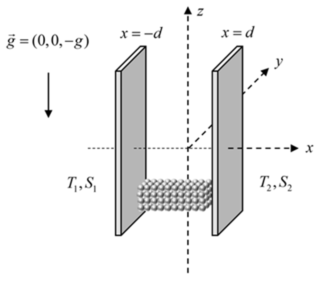
Figure 2.
Basic velocity profiles for different values of (a)RaT=100, RaS=50, (b)Da=0.1, RaS=50, (c) Da=0.1.
Figure 2.
Basic velocity profiles for different values of (a)RaT=100, RaS=50, (b)Da=0.1, RaS=50, (c) Da=0.1.
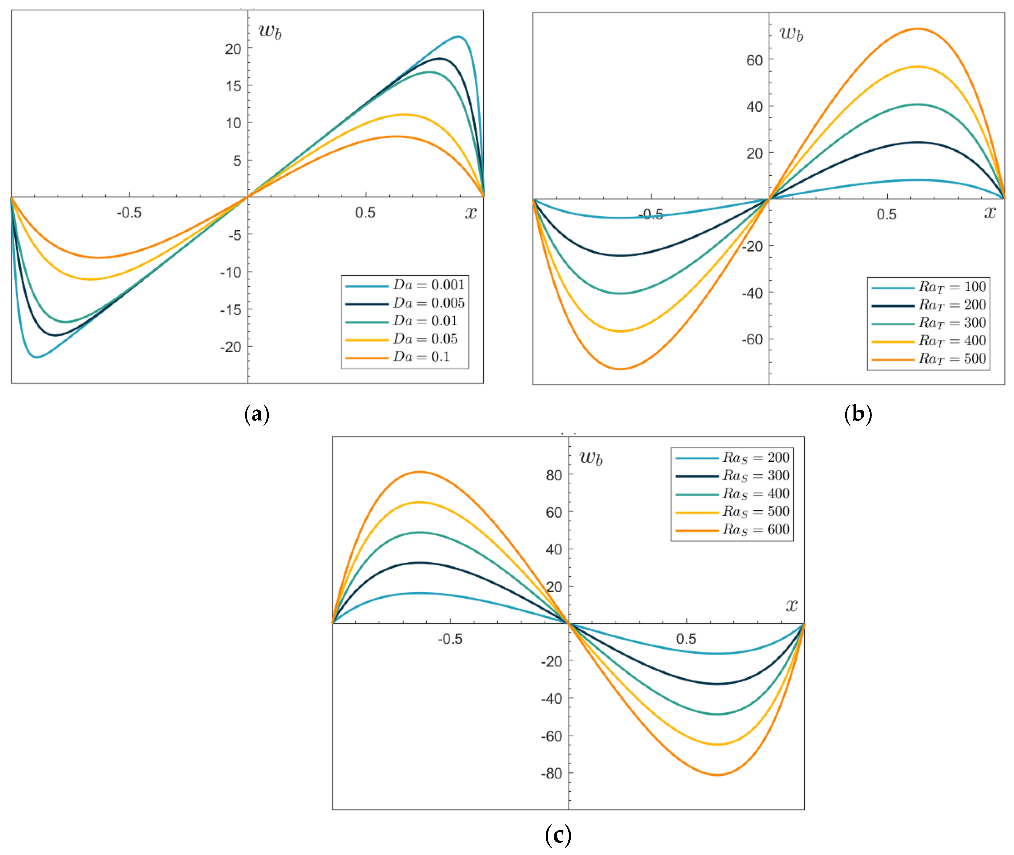
Figure 3.
Plots of the neutral stability curves and the growth rate for various values of (a)Le=1, (b)Le=1, RaT=1750, (c)Le=2, (d)Le=2, RaT =1750, when Da=0.1, PrD=50, λ1=0.4, λ2=0.2, Le=2, RaS=50, η=0.5.
Figure 3.
Plots of the neutral stability curves and the growth rate for various values of (a)Le=1, (b)Le=1, RaT=1750, (c)Le=2, (d)Le=2, RaT =1750, when Da=0.1, PrD=50, λ1=0.4, λ2=0.2, Le=2, RaS=50, η=0.5.
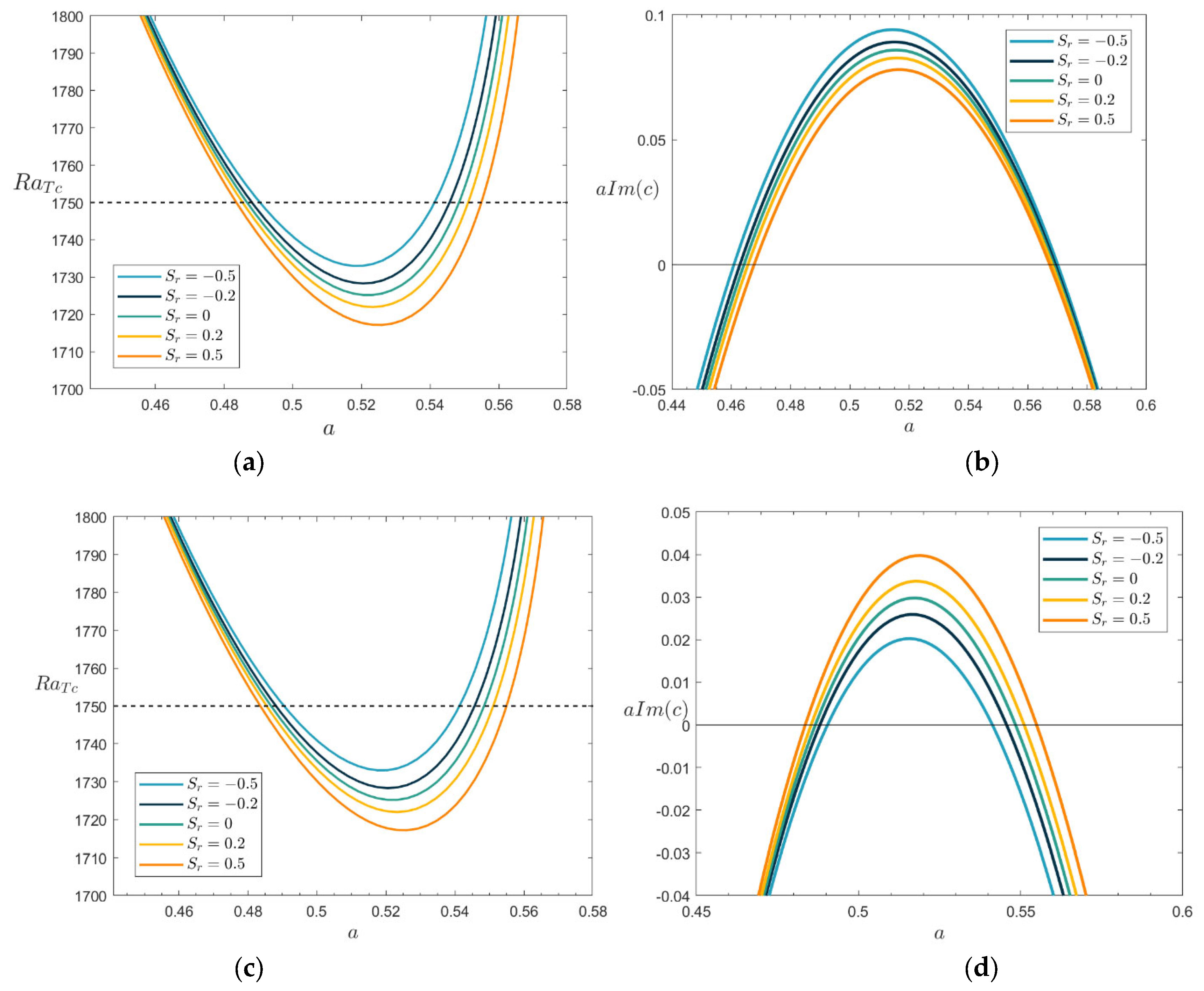
Figure 4.
Plots of the neutral stability curves and the growth rate when Da=0.1, PrD=50, λ1=0.4, λ2=0.2, Sr=-0.5, RaS=50, RaT=1750, η=0.5.
Figure 4.
Plots of the neutral stability curves and the growth rate when Da=0.1, PrD=50, λ1=0.4, λ2=0.2, Sr=-0.5, RaS=50, RaT=1750, η=0.5.
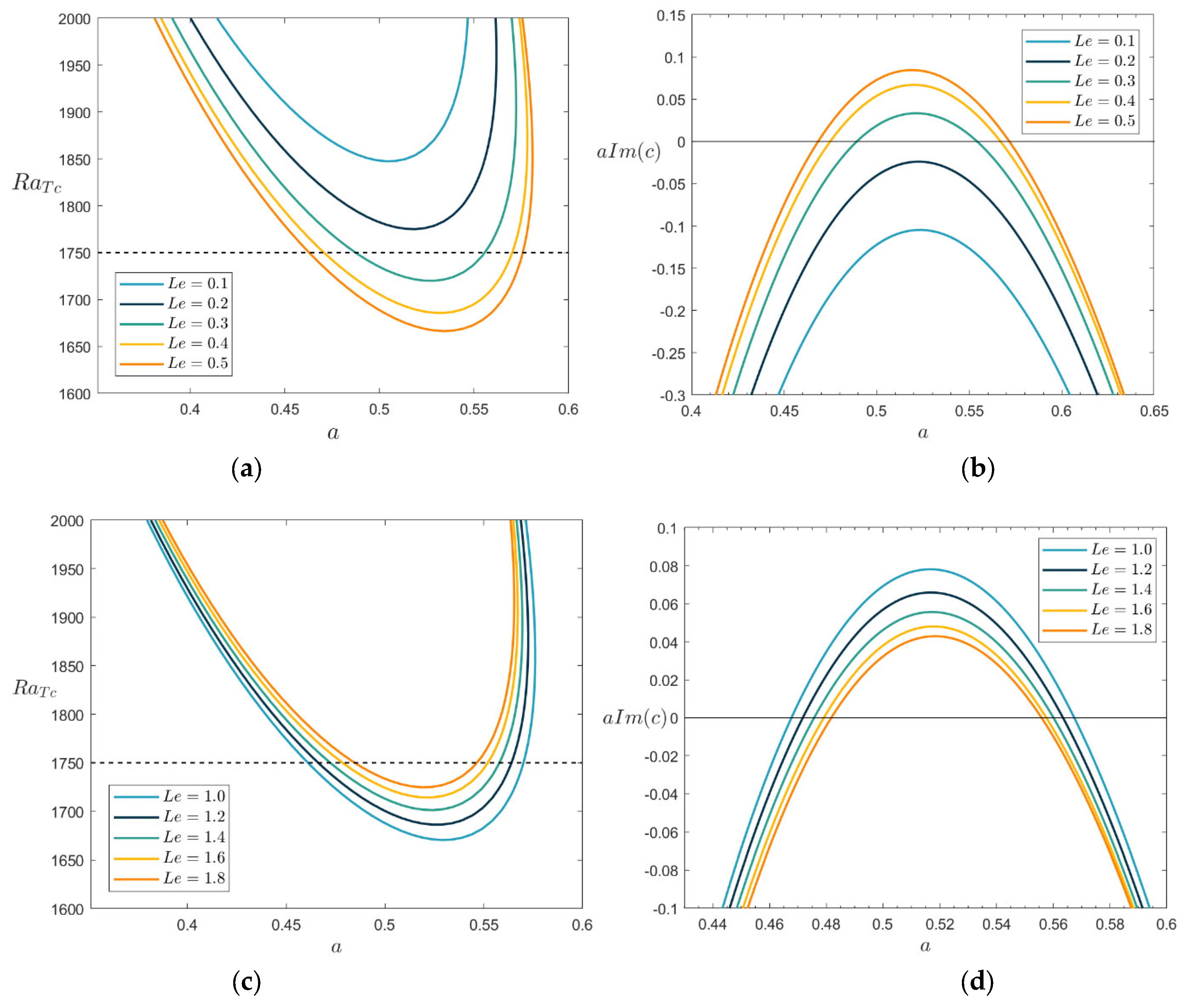
Figure 5.
Plots of the neutral stability curves when Da=0.1, PrD=50, λ1=0.4, λ2=0.2, RaS=50, η=0.5, a=0.5.
Figure 5.
Plots of the neutral stability curves when Da=0.1, PrD=50, λ1=0.4, λ2=0.2, RaS=50, η=0.5, a=0.5.
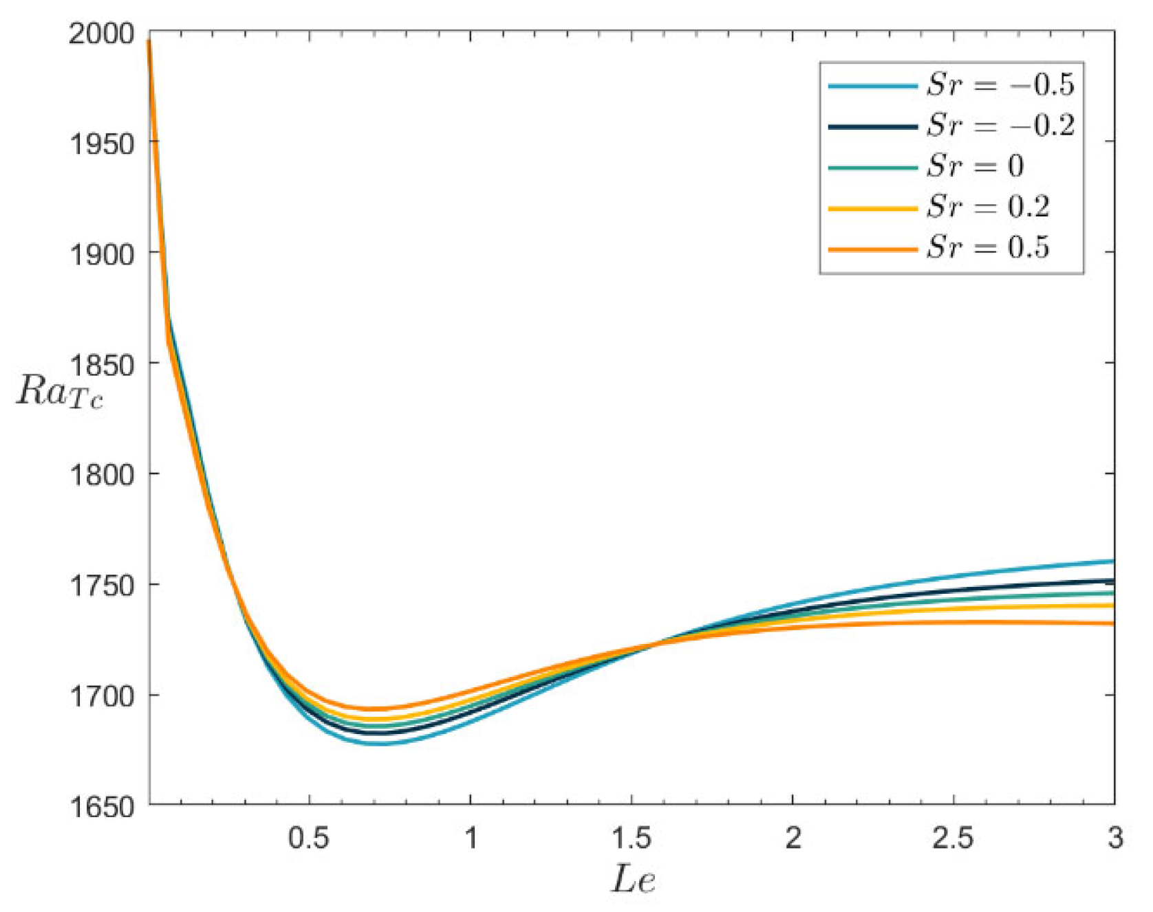
Figure 6.
Plots of the neutral stability curves and the growth rate when Da=0.1, PrD=100, λ1=0.4, λ2=0.2, RaS=50, η=0.5, Le=2, (b) RaT=1130, (d) RaT=1030.
Figure 6.
Plots of the neutral stability curves and the growth rate when Da=0.1, PrD=100, λ1=0.4, λ2=0.2, RaS=50, η=0.5, Le=2, (b) RaT=1130, (d) RaT=1030.
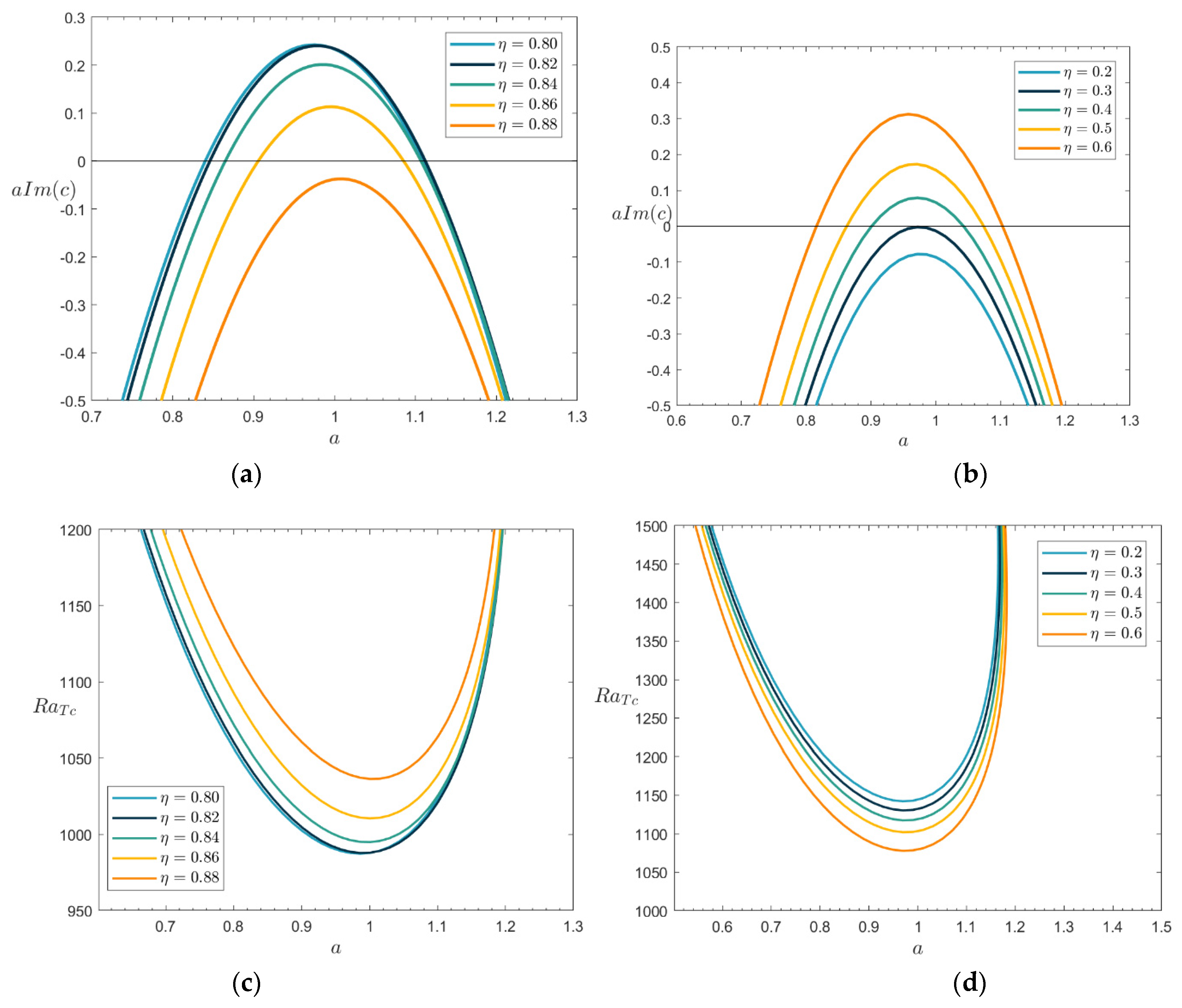
Figure 7.
Plots of the neutral stability curves and the growth rate. (a) Da=0.1, PrD=100, λ1=0.4, λ2=0.2, RaS=50, Le=2, Sr=0.5, a=π/4, (b) Da=0.1, PrD=100, λ1=0.4, λ2=0.2, RaS=50, Le=2, Sr=0.5, a=π/4, RaT=1400.
Figure 7.
Plots of the neutral stability curves and the growth rate. (a) Da=0.1, PrD=100, λ1=0.4, λ2=0.2, RaS=50, Le=2, Sr=0.5, a=π/4, (b) Da=0.1, PrD=100, λ1=0.4, λ2=0.2, RaS=50, Le=2, Sr=0.5, a=π/4, RaT=1400.
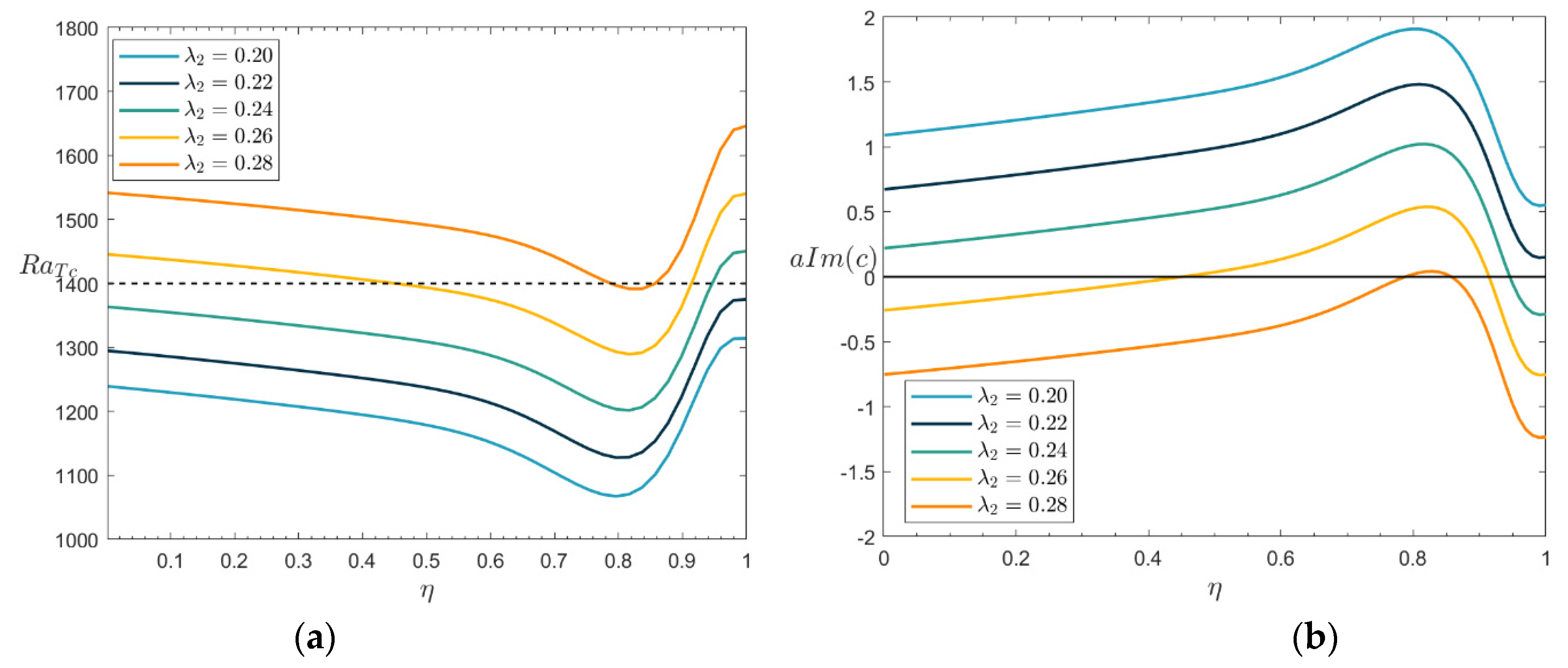
Figure 8.
Plots of the neutral stability curves and the growth rate for different values of (a) PrD=50, (b) PrD=200, (c) PrD=600, (d)a=π/10, when Da=0.1, Le=2, λ2=0.2, RaS=50, η=0.5, Sr=0.5.
Figure 8.
Plots of the neutral stability curves and the growth rate for different values of (a) PrD=50, (b) PrD=200, (c) PrD=600, (d)a=π/10, when Da=0.1, Le=2, λ2=0.2, RaS=50, η=0.5, Sr=0.5.


Table 1.
The Chebyshev collocation method's convergence process when Da=0.1, λ1=0.4 λ2=0.2, Le=2, PrD=100, RaT=1800, RaS=50, η=0.5, Sr=0.5.
Table 1.
The Chebyshev collocation method's convergence process when Da=0.1, λ1=0.4 λ2=0.2, Le=2, PrD=100, RaT=1800, RaS=50, η=0.5, Sr=0.5.
| The growth rateaci | |||
| N | a=0.5 | a=1 | a=1.5 |
| 30 | 1.371890 | 2.653114 | -3.712508 |
| 35 | 1.371895 | 2.653438 | -3.712476 |
| 40 | 1.371895 | 2.653448 | -3.712474 |
| 45 | 1.371895 | 2.653448 | -3.712474 |
Table 2.
Critical values of Lewis number Lec when Da=0.1, PrD=50, λ1=0.4, λ2=0.2, RaS=50, RaT=1750, η=0.5.
Table 2.
Critical values of Lewis number Lec when Da=0.1, PrD=50, λ1=0.4, λ2=0.2, RaS=50, RaT=1750, η=0.5.
| Sr | Critical values of Lewis number Lec1 | |
| a=0.4 | a=0.5 | |
| -0.5 | 0.7578 | 0.7147 |
| -0.2 | 0.7525 | 0.7106 |
| 0 | 0.7485 | 0.7066 |
| 0.2 | 0.7431 | 0.7025 |
| 0.5 | 0.7357 | 0.6944 |
Table 3.
Critical values of normalized porosity ηc when Da=0.1, PrD=100, λ1=0.4, λ2=0.2, RaS=50, η=0.5, Le=2, Sr=0.5.
Table 3.
Critical values of normalized porosity ηc when Da=0.1, PrD=100, λ1=0.4, λ2=0.2, RaS=50, η=0.5, Le=2, Sr=0.5.
| Critical values of normalized porosity ηc | |||
| λ2 | a=π/6 | a=π/5 | a=π/4 |
| 0.2 | 0.7895 | 0.7908 | 0.7966 |
| 0.22 | 0.7969 | 0.7990 | 0.8057 |
| 0.24 | 0.8051 | 0.8071 | 0.8118 |
| 0.26 | 0.8112 | 0.8153 | 0.8209 |
| 0.28 | 0.8194 | 0.8215 | 0.8270 |
Disclaimer/Publisher’s Note: The statements, opinions and data contained in all publications are solely those of the individual author(s) and contributor(s) and not of MDPI and/or the editor(s). MDPI and/or the editor(s) disclaim responsibility for any injury to people or property resulting from any ideas, methods, instructions or products referred to in the content. |
© 2024 by the authors. Licensee MDPI, Basel, Switzerland. This article is an open access article distributed under the terms and conditions of the Creative Commons Attribution (CC BY) license (http://creativecommons.org/licenses/by/4.0/).
Copyright: This open access article is published under a Creative Commons CC BY 4.0 license, which permit the free download, distribution, and reuse, provided that the author and preprint are cited in any reuse.


