
Submitted:
31 October 2024
Posted:
01 November 2024
You are already at the latest version
Abstract
A home-built equipment will be presented able to measure thermal expansion and indentation up to 1100 oC. The principle of operation is similar to that of Rockwell hardness measurement. First, we apply a small load and measure the thermal expansion of the construction consisting of the sample holder quartz tube, the conical in-denter and the sample. Then we repeat the thermal cycle with such a high load that produces a deviation in thermal expansion already after 200-300 oC, compared to the previous thermal expansion measurement with low load. With increasing temperature, the indentation depth increases and at higher temperatures we already notice a contraction. The evolution of indentation depth as a function of temperature, d(T), we can obtain by sub-tracting the high load curve from the low load curve. Newly created phenomenological expressions will be tested to describe the thermal softening of pure metals and refractory HEAs. The results will be interpreted taking into account the allotropic transformations and temperature dependencies of elastic moduli. We are working on the instrument to extend the working temperature up to 1200 oC.
Keywords:
temperature dependence of mechanical properties
; elastic moduli
; yield stress and hardness
; thermal expansion
; softening and allotropic phase transformations
; refractory high entropy alloys
1. Introduction
In practice, the mechanical resistance against high temperature softening should be measured and characterized through the temperature dependence of mechanical parameters like elastic moduli , yield stress and hardness. It is difficult and costly to create experimental environment and measuring technique around and above 1000 degree Celsius. Phenomenological models of mechanical characteristics can lead to financial and time savings. Therefore, a short review of the theoretical; models and formulas will be presented concerning the temperature dependence of elastic moduli, yield stress and hardness.
A good compendium about the elastic modulus estimation models was presented by Weiquo Li et al.[1]. His formulas follows the general adopted form, the values at different temperatures are given with reference of parameter value at zero absolute temperature:
where α is the linear thermal expansion coefficient, ∆fusH is the heat of fusion and Cv is the specific heat capacity. This rational fraction expression was furthermore simplified by Zakarian et al. [2] deducing the following “universal “ temperature dependence for elastic (Young) modulus:
Where, Eo – is the elastic modulus at zero temperature,
Tm – is the melting point of the material.
We have checked the „universality” of eq. (2), using the experimental E versus T data collections of [3] and we have found no matching with the calculated data. Even more, instead of theoretically predicted concave curve, the experimental points follow a convex curve in the case of Titanium. The only advantage of “universal” curve is that describe correctly the value of E at melting point. inserting T = Tm in Eq. (2), we obtain the correct value of E at Tm which is 55% of the initial value not zero as it was supposed by Born [4] based on theoretical considerations, before having the experimental data. Consulting the experimental data it turned out that the supposition about the vanishing C44 at melting was not correct. Instead, it preserve 55 % of its maximal value at zero K, C44(Tm)= 0.55*C44(0)
Concerning the temperature dependence of yield stress we cite here Z. Wu et al. [5], who revived the idea of Dietze [6] about the temperature dependence of yield stress which is the same as that of the Peierls stress, and obtained the yield stress exponentially decaying with temperature:
where ω is the dislocation width, which depend linearly from the absolute temperature, the proportionality factor being 1/Tm and b is the Burgers vector.
Others have taken another route [5], assuming that yielding at temperature T occurs when the sum of the elastic deformation energy per unit volume and the corresponding heat energy reaches a certain value. The ratio of the yield stresses at temperature T compared to its initial value can be calculated without free parameters using the tabulated values of specific heat capacities and of elastic moduli:
Although both temperature dependencies are related to the hardness they are not the same. The main difference is that at melting temperature about 0,55 part of modulus is still present whereas the yield stress (together with the hardness) decay down to zero.
Even more, the yield stress (YS) scales with the Vickers hardness (HV) at around room temperature, they are related by the well known three-time relations [7, 8]:
HV = 3*YS
In general, the variation of hardness (HV) with T is very characteristic: at small temperatures HV is practically constant and as the temperature of the material increases, hardness decreases and at some point a drastic change in hardness occurs. The hardness at this point is termed the hot or red hardness of that material. Such changes can be seen in materials such as heat - treated alloys. Precipitation hardening may overlap with red hardness behavior, this is why special attention is needed to separate them.
The first reliable high-temperature Vickers hardness data (up to 800 oC) were published in 1950 years [9] although, the formula of variation of hardness with temperature was already published by Ito [10]:
H(T)/H(To) = exp(-BT),
where H(To) is the intrinsic hardness, and B is the softening coefficient of hardness. These two parameters change after the red hardness point. Considering the three -time relation (5) ,we can accept the explanation given for the temperature dependence of yield stress valid for the equation (6) of hardness as well.
Westbrook [9] proposed another model to describe the hardness versus temperature, which is similar to the Ito–Shishokin model. The model is shown as follows:
where A′ and B′ are constants, which also have one set of values at low temperature and another set at high temperature. Westbrook model can be derived based on the Arrhenius equation [Merchant]. nevertheless non of the two models can be extrapolated to predict the hardness values at lower and higher temperatures. It seems evident that equations (6) and (7) can not be valid in the same time for the same sample In this work, we try to clear up the validity of T dependence relationships and eventually propose a new phenomenological formula.
All the single-phase alloys and compound showed a common feature of temperature dependence of hardness: a slight decrease to two-thirds of the melting point followed by a drastic decrease indicating that the hardness mechanism had changed. We will refer to the change as “softening” in this work. The first scope of this work is to determine this softening temperature by a home built thermal displacement meter applying a Rockwell – type hardness data evaluation of indentation depth. The second scope of this work is to present a formula valid in the whole temperature interval and is specially suitable to provide the softening temperature, Ts, where the drastic change in HV happens.
2. Experimental
Searching the device market, one can find, for example, the Rtec high temperature hardness testing equipment of ST Instruments. The instruments provides indents in multiple locations up to 1200 oC and the relative large chamber permit mounting several samples at the same time (https://vimeo.com/313936085).
Nevertheless, the advantage of obtaining similar standard-like hardness data as at room temperature, is overshadowed by the slowness of the measurement, during which structural changes can take place at the high temperature of the measurement. To overcome this problem, in this work we propose a high heating rate home built device, with maximal heating rate of 35 K/min. The temperature - displacement data pairs are detected in every second during the heating up process. The data are stored on line and , in the same time, is presented on the screen.
The schematic drawing of the instrument is shown in Figure1.
All quartz around the specimen, the sample capture and indenter guide. See the inserted drawing on sample and indenter (positions: 4, 5, 8, 9)
Figure 1.
Schematic drawing of the softening measurement.
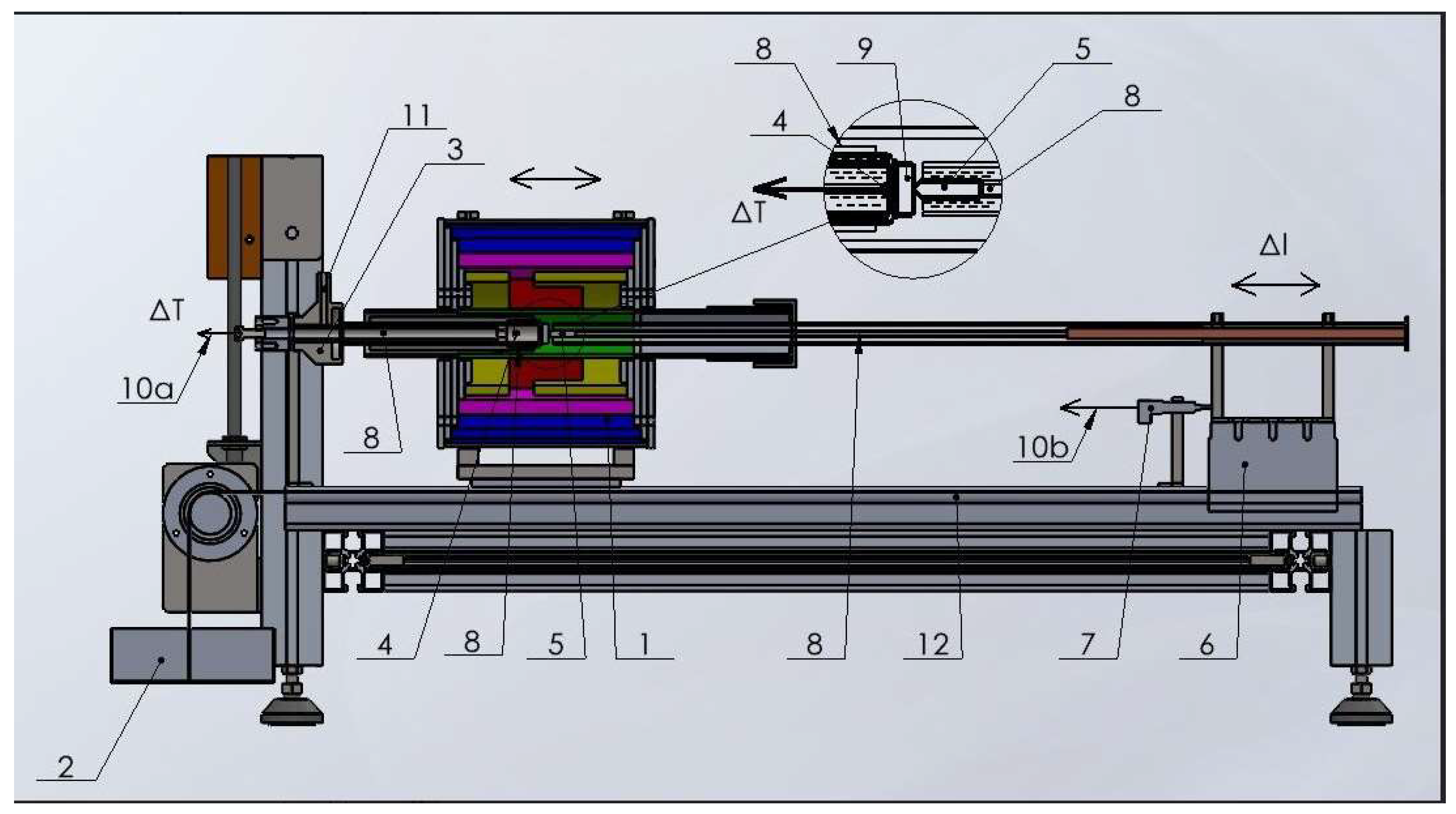
- tube furnace that can be shifted
- stressing load
- fix point for indentation measurement
- thermocouple
- indenter
- guide, moving unite gliding on ball bearings
- Inductive displacement sensor
- rods and tubes from quartz.
- sample
- a) sample temperature ( ΔT), 10.b) displacement of the indenter (Δl)
- Argon gas inlet,
- brittle rail structure
The sample can be a cube or a cylinder, should not be a regular form but it is essential to have two plan-parallel faces at a distance of about 5-20 mm, for fixed clamping. The section of the faces should be minimum 5 mm2 when we use a 1 mm diameter indenter. The sample (9) the indenter (5) and the clamping quartz tubes (8) form one corp under 0,5 kg stressing load. The measuring load is, in general, 1,5-3 kg. The resistive tubular furnace concentrates the heat around the sample, plus – minus 20 mm. It,s small size make possible high heating rate up to 35 K/min. The measurement is done under flowing argon. Home-made tungsten indenters have been prepared on
demand of particular material and sample size (see Figure 2 c). The trace of the indenter is shown in Figure2. d after1.5 kg and 0.5 kg loads.
Figure 2.
Operational form of the equipment. .
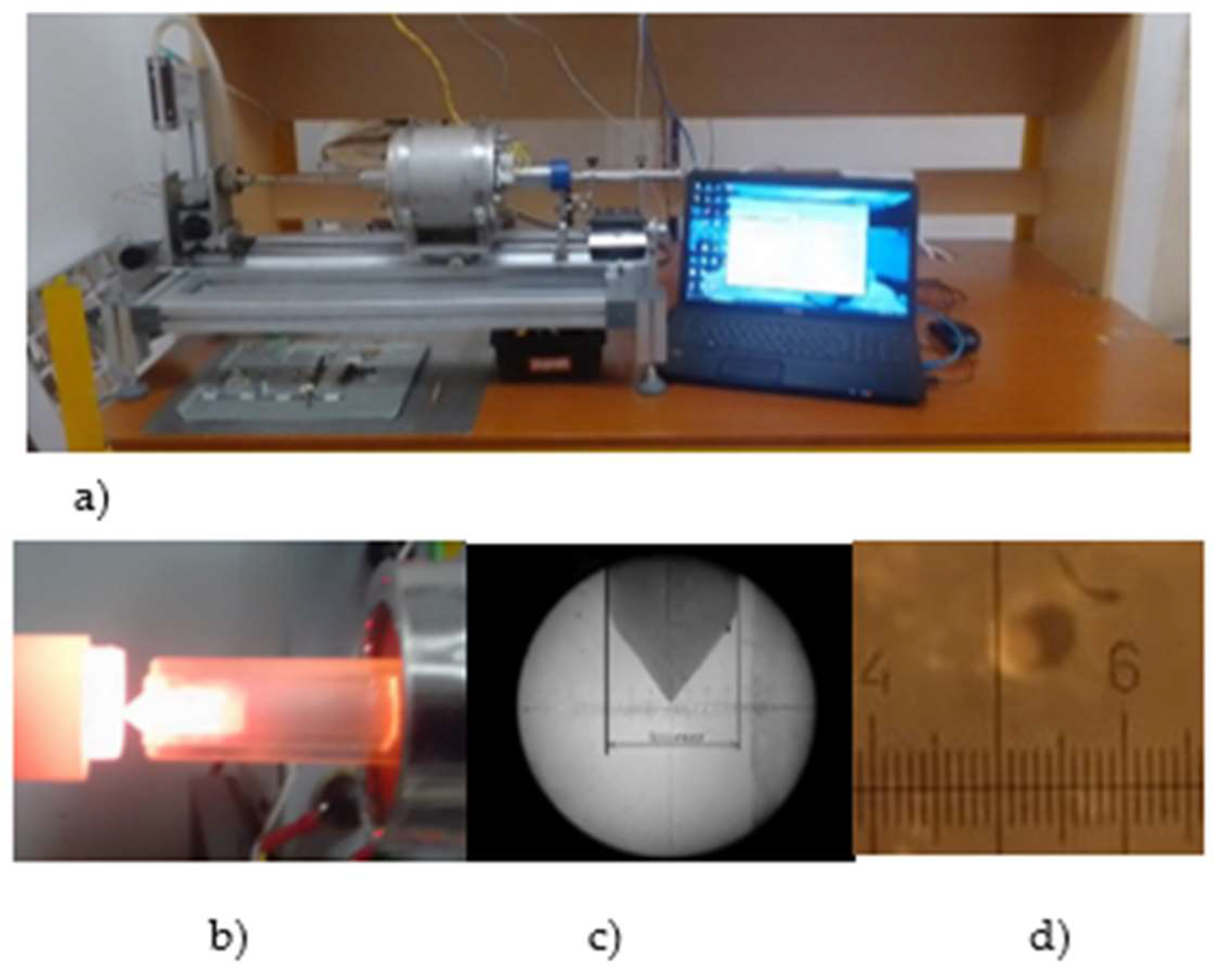
- a) overall view of the equipment,
- b) white – hot sample and indenter around 1000 oC without Ar protection (furnace is shifted), c) the W indenter tip preserving its form after several applications (1 div = 75 µm), d) indent views after indentation with 2,5 kg load.
3. Results and discussions
3.1. Measurement of Thermal Expansion and Related Thermal Transitions
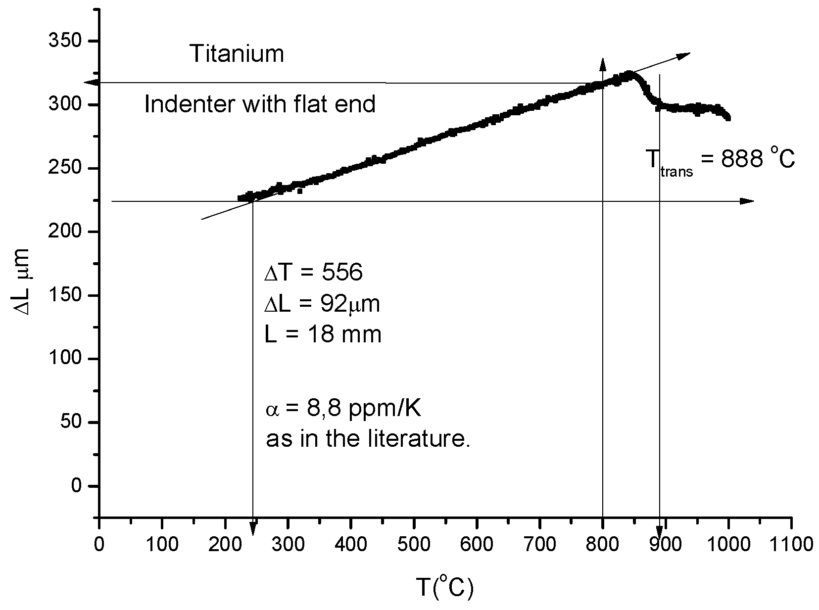
For thermal expansion measurements minimal load (0,5 kg) is applied and an indenter with flat end was prepared. During this type of measurements, no softening (i.e. no contraction) take place. More or less a linear displacement is measured. Should not be forgotten that the overall expansion coefficient includes beside the expansion of the sample, the expansion of the indenter and quartz tube as well. These latter expansions can be removed by careful calibration. Nevertheless the HCP - BCC phase transition of Titanium sample is clearly visible and can be used for temperature calibration (see Figure3).
Figure 3.
Linear thermal expansion of Titanium and phase transition at Ttr = 888 oC.
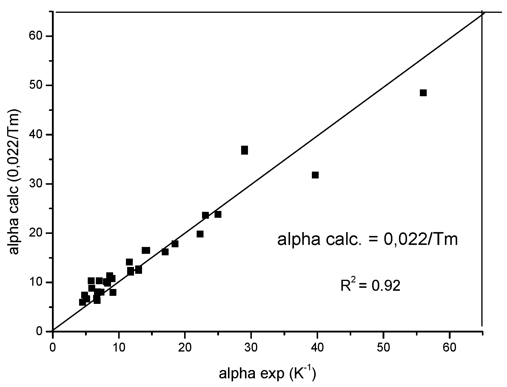
Driven by curiosity concerning the performance of our home built device, we measured the thermal expansion of some metals and found a good agreement with the literature data, what's more, we not only detected the phase transformations for the metals showing allotropic phase transformations (for example, Ti Zr, Fe and Co), but also found a good agreement between the measured and theoretical transformation temperatures, helping temperature calibration. We found an interesting correlation between the linear thermal expansion coefficient and the melting point: the average linear expansion coefficient above room temperature is invers proportional to the melting point (see Fig 4). The relation :
α = 0.022/Tm
was verified with R2 = 0.92 for 32 elemental metals based partly on own and partly on literature data. The discussion of this relationship need a separate article.
Figure 4.
The linear expansion coefficient scales with the reciprocal of melting temperature.
3.2. Measurement of Rockwell - Type Hardness as a Softening Meter
This time we use the pointed end tungsten indenter, and repeat the measurement with 0,5 kg load because this will be the reference curve. The starting temperatures and the heating rate should be the same for preload 0.5 kg and for the load of 1.5 kg. This time the positive displacement measured by the sensor turns on negative, indicating the drastic decrease of hardness at high temperatures. The details can be followed on Figure 5. First, we measure the displacement curves for a small load (0.5 kg in this case) and a larger load (1,5 kg) (see Fig 5a). The difference of these two curves will give the indentation depth (ID) and the Rockwell -type hardness will be obtained (Figure 5b) by subtracting the indentation depth from an arbitrarily chosen number:
After this short presentation of the home built instrument we can observe the following advantages compared to the commercial available one: 1) High heating rate (short duration of the measurement) makes possible to avoid the precipitation of phases from the supersaturated solid solution structure of the refractory high entropy alloys. 2) irregular shape samples, having two plan parallel faces only can be measured, no need for standard form samples as in the case of commercial device. 3) beside the hardness type measurements, it is possible to measure the thermal expansion together with its thermal dependence and, in addition, can be studied the phase transition as it appears in thermal dilatation. This means that our device works as a dilatometer as well. 4) The quick measurement enables series measurement’s which might be important in a production unit, 5) Last but not least our home built device is order of magnitude cheaper than the commercial device.
In Figure 6 we are presenting the extraction of Rockwell - type hardness from softening measurements under a pre-load of 0,5 kg and a load of 1,5 kg.
The measured displacement is a sum of the positive dilatation and negative indentation depth. The hardness (HR) is proportional to the indentation depth (ID). We present two methods for determining ID:
1)- First, we measure the displacement curves (D) for different loads (see Fig 6a). In the spirit of Rockwell type hardness measurement, we determine the indentation depth (ID) by subtracting two displacement data: those got with bigger load (1 and 3 kg) from those got with small one (0.5 kg). The increasing ID is transformed in a decreasing HR by simple subtraction of ID from an arbitrarily chosen value (300), (see eq. 9):
- The softening temperature (Ts = 950 K) is assessed to the “knee” point of the HR(T) curve( see Figure6.b). This hot-red point is visible displacing to smaller values with increasing load. The optimal load should be chosen as a function of initial, low temperature hardness, taking into account that the larger the load the more difficult to perform the measurement.
2) For rapid measurements we propose the following protocol.:
- - taking into account that the thermal expansion coefficient, TEC , has a small and negligible increase with temperature, we take as an average TEC the low temperature value and construct in Figure7, the thermal expansion line (see Figure 7a). The indentation depth (ID) is obtained by subtracting the measured displacement (D) curve from the thermal the expansion line (TEL):TEL - D = ID
Finally, we obtain the hardness in Figure 7b. with the equation (8).
We end up this section by presenting the softening measurement on refractory high entropy alloys presented in Table1. The samples were prepared in our lab by inductive melting in water cooled copper mold. Beside the composition some important material characteristics are collected in Table 1 to help interpreting the measured softening temperature (Ts) data.
To obtain the Rockwell type hardness we have applied the rapid measurement technique presented above. We are not going to present again all the steps of the measuring protocol, except two samples. The sample number 4 is characteristic in general for refractory HEAs (Figure 8) and sample number 2 (TiZrHf) which shows a double stage decrease as a function of temperature (Figure 9)
The double stage temperature dependence of hardness for our sample number 2 consisting from 3 metals (TiZrHf) with allotrope transformations around 800-900 oC is revealed better after presenting the RH(T) curve (see Figure 9b) calculated from the measured D(T) curve(see Figure 9a).
- a)
- the parameter ID is calculated following the protocol described above
- b)
- the hardness calculated from 150-ID shows beyond doubt the phase transformation around 800-900 oC where the second softening starts. The first softening happens at a surprisingly low temperature, Ts1 = 450 oC
In fig 10 we present the measured displacement data (see Fig 10a and the calculated Rockwell type hardness for our refractory HEAs samples.
In general, the visually determined softening temperature is about half of the melting temperature:
Ts = Tm/2
This relation is verified for the pure metal except those presenting allotrope transformations (see Figure 11). In the case of metals presenting allotrope transition the thermal softening temperature decrease to the half of the transition temperature which is much lower than the half of the melting point. It turns out that for true refractory alloy with high softening temperature we have to design a structural stable alloy composition.
Unfortunately, the equations describing the temperature dependence of hardness have a pure goodness- of- the- fit (R2) measure in the case of RHEAs. Looking for a better phenomenological equation we came across the following expression
where H(To) is the reference hardness at room temperature and Tc is the characteristic temperature and n is the exponent to be fitted. The Tc and n pair data were determined for all the 8 our samples and are presented in Table 1. The goodness of the fit, R2, was always above 0.9.
The characteristic temperature Tc is the temperature where the hardness drop off to half of its room temperature value (for T = Tc equation (12) gives a ratio ½.) In general, Tc is larger with several hundred degree compared to the Ts determined visual. This is why our formula permits prediction of hardness in high temperature region as well.
4. Conclusions
- Measurement with a commertialized equipment is equivalent with a heat treatment which may influence the valadity of high temperature meaurements. Here we present a relative rapid measurement reaching the maximum temperature( 1100 oC) within half an hour.
- Due to the high heating rate all the nonequilibrium alloys (amorphous, over-saturated solid solution, like HEA can be studied in „as received” state suppressing or eliminating the time dependent diffusional effects
- Detailed meauement protocol was presented to facilitate determination and evaluation of high temperature hardness measurement.
- The presented device serve as dilatometer as well, applying the necessary corrections for the dilatation of quartz tube and tungsten indenter.
- The presented device is order of magnitude cheeper than those commertial available
- The presented device is easy to build up in even a moderately equipped lab.
- New formula was presented , permitting to fit the experimental results in the whole temperature range
Author Contributions
Otto K. Temesi: writing – original draft, data curation , Albert Karacs: manufactoring the device, supervision, validation, writing -editing Lajos K. Varga: conceptualization, writing - original draft, review and editing, Nguyen Q, Chinh: formal analysis, writing – review editing. The link for defining the role of authors and contributors: https://www.icmje.org/recommendations/browse/roles-and-responsibilities/defining-the-role-of-authors-and-contributors.html
Funding
This research was funded by Government of Hungary for the support from the Market-driven R&D and Innovation grant (2020-1.1.2-PIACI-KFI-2020-00025).
Data Availability Statement
The data that support the findings of this study are partly taken from the cited references
Acknowledgments
Thanks to the Government of Hungary for the support from the Market-driven R&D and Innovation grant (2020-1.1.2-PIACI-KFI-2020-00025).
Conflicts of Interest
The authors declare that the research was conducted in the absence of any commercial or financial relationships that could be construed as a potential conflict of interest.
References
- Weiguo Li, Haibo Kou, Xuyao Zhang, Jianzuo Ma, Ying Li, Peiji Geng, Xiaozhi Wu,Liming Chen, Daining Fang, Temperature-dependent elastic modulus model for metallic bulk materials, Mechanics of Materials 139 (2019) 103194. [CrossRef]
- D. Zakarian ⇑, A. Khachatrian, S. Firstov, Universal temperature dependence of Young’s modulus, Metal Powder Report d Volume 74, Number 4 d July/August 2019.
- Wu, H. Bei, G.M. Pharr, E.P. George, Temperature dependence of the mechanical properties of equiatomic solid solution alloys with face-centered cubic crystal structures, Acta Materialia, Volume 81, December 2014, Pages 428-441. [CrossRef]
- M. Born and K. Huang, Dynamical Theory of Crysta Lattices (Oxford U. P., Oxford, England, 1954).
- Z. Wu, H. Bei , G.M. Pharr a,b, E.P. George, Temperature dependence of the mechanical properties of equiatomicsolid solution alloys with face-centered cubic crystal structures, Acta Materialia 81 (2014) 428– 44. [CrossRef]
- Horst-Dietrich Dietze. (1952). Die Temperaturabhängigkeit der Versetzungsstruktur., 132(1), 107–110. [CrossRef]
- Weiguo Li, Xianhe Zhang, Haibo Kou, Ruzhuan Wang , Daining Fang, Theoretical prediction of temperature dependent yield strength for metallic materials , International Journal of Mechanical Sciences 105 (2016) 273–278. [CrossRef]
- E.J. Pavlina and C.J. 8: Van Tyne, Correlation of Yield Strength and Tensile Strength, with Hardness for Steels, Journal of Materials Engineering and Performance, JMEPEG (2008) 17, 2008. [CrossRef]
- Westbrook, J. H.. (1957). Temperature dependence of the hardness of secondary phases common in turbine bucket alloys. JOM, 9(7), 898–904. [CrossRef]
Figure 5.
a) Titanium under 0.5 kg and 1,5 kg load. The red hardness point (Tm/2) was found to be around the phase transition temperature. b) Determination of Rockwell type (RH) hardness as RH = 300- ID.
Figure 5.
a) Titanium under 0.5 kg and 1,5 kg load. The red hardness point (Tm/2) was found to be around the phase transition temperature. b) Determination of Rockwell type (RH) hardness as RH = 300- ID.
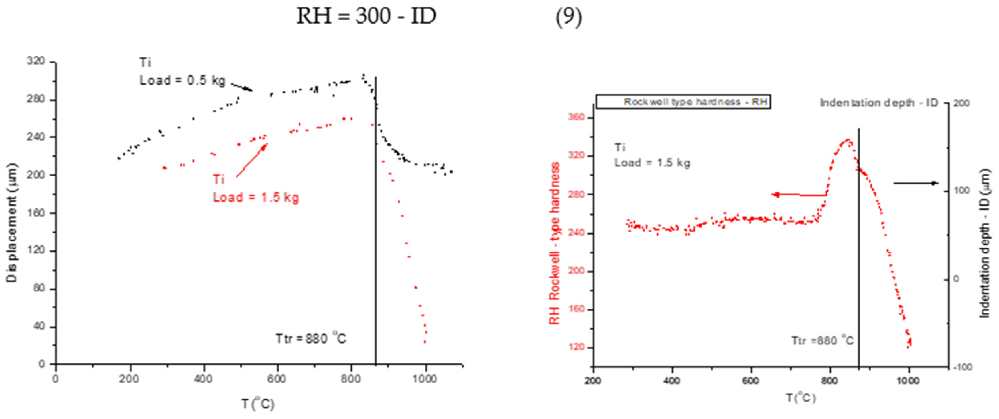
Figure 6.
Softening measurement with high heating rate (30 K/min) on pure iron. a) displacement measurement as a function of loads. b) Rockwell type hardness as a function of temperature.
Figure 6.
Softening measurement with high heating rate (30 K/min) on pure iron. a) displacement measurement as a function of loads. b) Rockwell type hardness as a function of temperature.
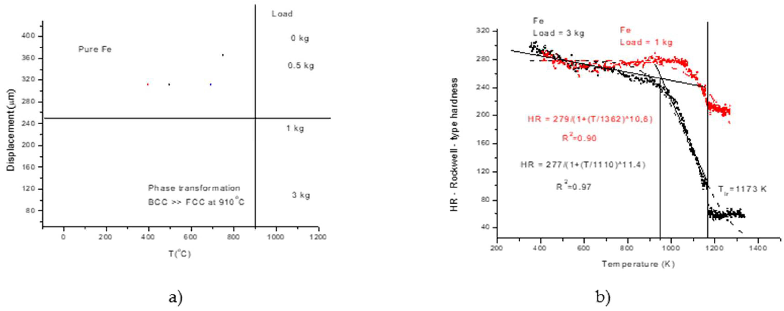
Figure 7.
Rapid evaluation protocol for softening measurement on Fe. a) Construction of thermal expansion line (TEL) based on the initial part of the measured displacement curve (D) b) Representing the indentation depth obtained as ID = TEL – D and the corresponding Rockwell-type hardness RH = 300 -ID.
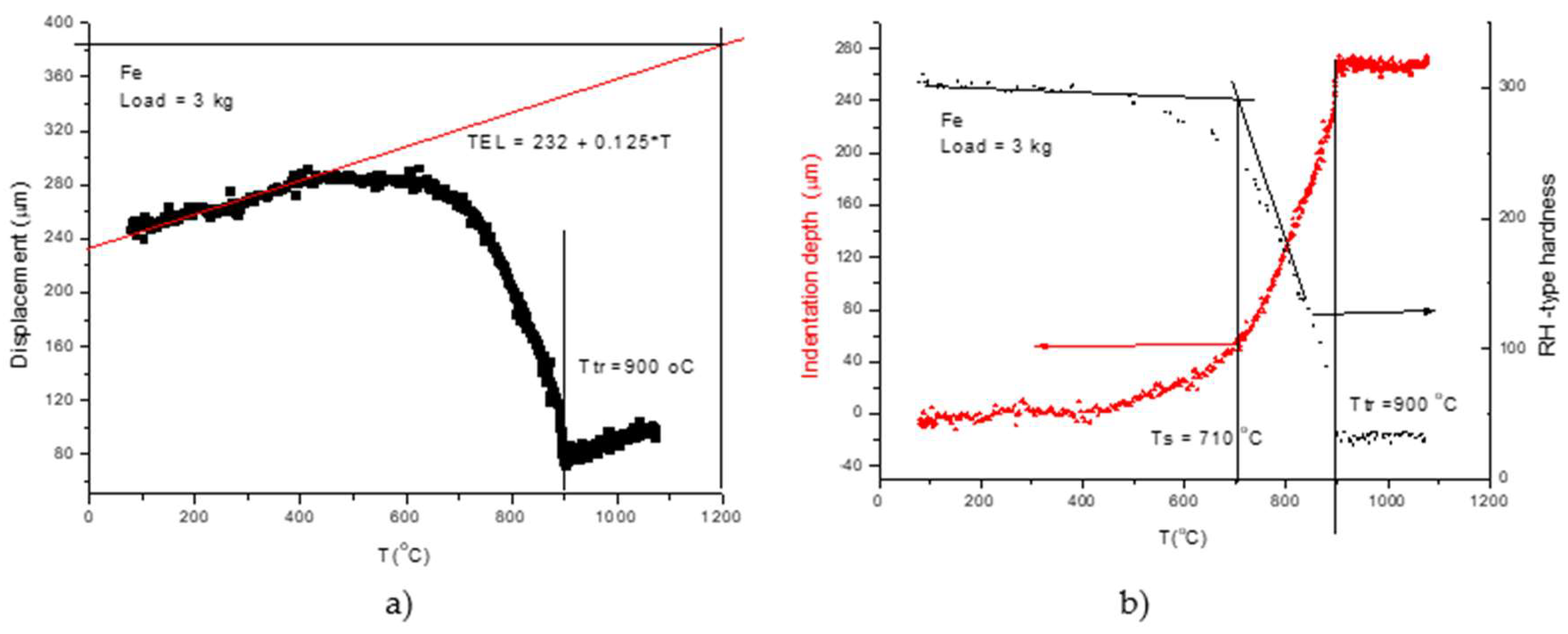
Figure 8.
Thermal softening measurement on TiZrHfNb refractory HEA. a) presents the original displacement measurement (D), the thermal expansion line (TEL) determined from extrapolation of the initial part of D versus T curve, and indentation depth (ID) obtained by subtraction ID = TEL-D. b) Rockwell type hardness determined by subtraction RH = 200 – ID and the softening Ts temperature determination only visually from the intersection of two tangent lines.
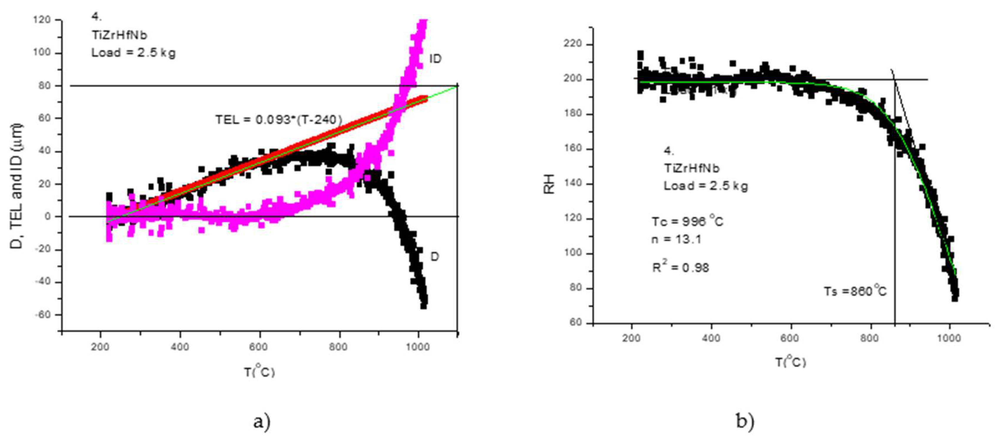
Figure 9.
Thermal softening measurement on TiZrHf refractory HEA.
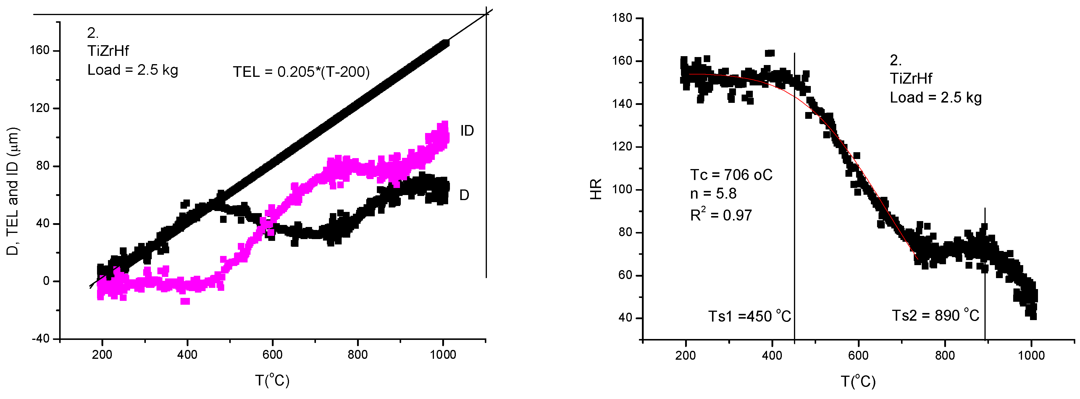
Figure 10.
Thermal softening measurements on our refractory HEAs samples (see data in Table 1)a) measured displacement data, b) calculated RH data. .
Figure 10.
Thermal softening measurements on our refractory HEAs samples (see data in Table 1)a) measured displacement data, b) calculated RH data. .
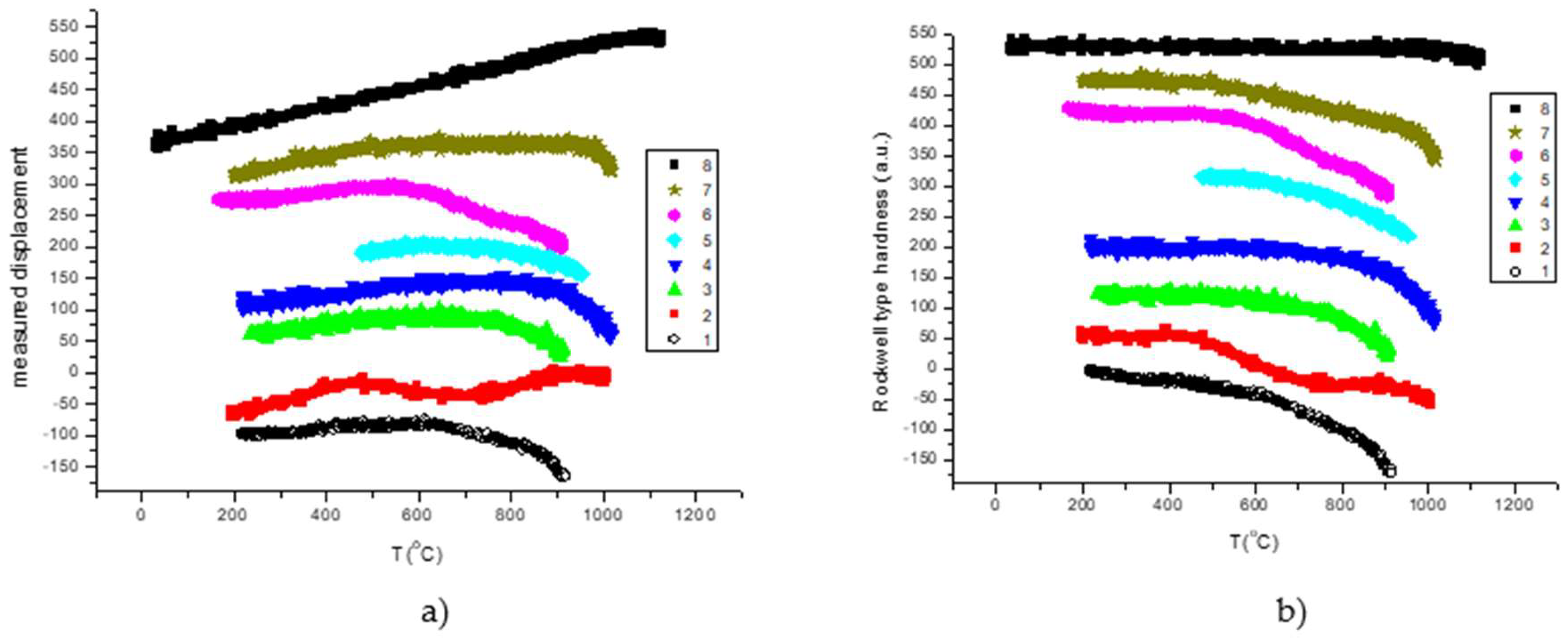
Figure 11.
Thermal softening temperature for pure metals equals to the half of melting point.
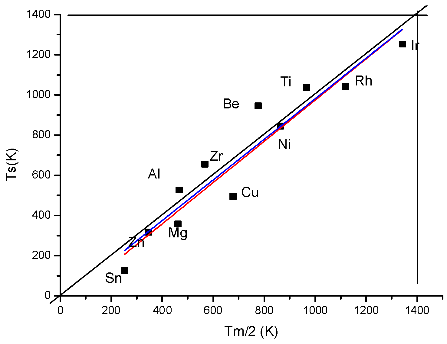

Table 1.
Data of investigated refractory high entropy alloys.
| RHEA | a(Angstrom) | VEC | HV (kgf/mm2 | Ts (oC) |
Tc (oC) |
n | |
| 1 | Y25Ti25Zr25Hf25 | 3.57702 | 3.75 | 271.3 | 610 | 823 | 5.53 |
| 2 | Ti33.33Zr33.33Hf33.34 | 3.47057 | 4 | 310.16 | Ts1 =450 Ts2 = 890 |
706 | 5.8 |
| 3 | Ti30Zr30Hf30Nb10 | 3.45071 | 4.1 | 336.46 | 722 | 803 | 11 |
| 4 | Ti25Zr25Hf25Nb25 | 3.42335 | 4.24 | 336.21 | 860 | 996 | 13.1 |
| 5 | Ti25Zr25Hf25Nb25 | 3.42335 | 4.4 | 415.19 | 744 | 830 | 10.8 |
| 6 | Ti25Zr25V25Nb25 | 3.29035 | 4.5 | 381.16 | 520 | 758 | 8 |
| 7 | Ti20Zr20V20Nb20Ta20 | 3.30111 | 4.6 | 398.71 | 1000 | 1004 | 4.91 |
| 8 | V25Nb25Mo25W25 | 3.17187 | 5.5 | 432.24 | 1000 | 1250 | 12.5 |
Disclaimer/Publisher’s Note: The statements, opinions and data contained in all publications are solely those of the individual author(s) and contributor(s) and not of MDPI and/or the editor(s). MDPI and/or the editor(s) disclaim responsibility for any injury to people or property resulting from any ideas, methods, instructions or products referred to in the content. |
© 2024 by the authors. Licensee MDPI, Basel, Switzerland. This article is an open access article distributed under the terms and conditions of the Creative Commons Attribution (CC BY) license (http://creativecommons.org/licenses/by/4.0/).
Copyright: This open access article is published under a Creative Commons CC BY 4.0 license, which permit the free download, distribution, and reuse, provided that the author and preprint are cited in any reuse.


