Asymptotic and Probabilistic Perturbation Analysis of Controllable Subspaces

In this paper, we consider the sensitivity of the controllable subspaces of single-input linear control systems to small perturbations of the system matrices. The analysis is based on the strict componentwise asymptotic bounds for the matrix of the orthogonal transformation to canonical form, derived by the method of the splitting operators. The asymptotic bounds are used to obtain probabilistic bounds on the angles between perturbed and unperturbed controllable subspaces implementing the Markoff inequality. It is demonstrated that the probability bounds allow to obtain sensitivity estimates which are much tighter than the usual deterministic bounds. The analysis is illustrated by a high order example.

Keywords:

Subject:

Computer Science and Mathematics - Computational Mathematics

MSC: 47A55; 93C05; 93C73; 93B05; 65F25

1. Introduction

The notion of controllable subspace plays an important role in linear control theory [26]([Ch. 1]), [7]([Ch. III]). In this paper we are interested in the sensitivity to small parameter perturbations of the controllable subspaces of single-input time-invariant linear control systems, described by the state equation

\dot{x} (t) = A x (t) + B u (t),

(1)

where

x \in R^{n}

is the state vector,

u \in R^{1}

is the control vector and

A \in R^{n \times n}, B \in R^{n \times 1}

. The subspace

C_{k} = \sum_{j = 1}^{k - 1} A^{j} R (B) = R ([B, A B, \dots, A^{k - 1} B]), k = 1, 2, \dots, n

is said to be the kth controllable subspace of (1). Clearly,

\dim (C_{k}) = rank ([B, A B, \dots, A^{k - 1} B]) .

We have that

C_{1} \subset C_{2} \subset \dots \subset C_{n} .

The subspace

C_{n}

is said to be the controllable subspace of the pair

(A, B)

. If

\dim (C_{n}) = n

, i.e.,

C_{n}

is the whole state space, then the system (1) and respectively the pair

(A, B)

, is called controllable. If the system is controllable, then for every vector

x_{T} \in C_{n}

and

T > 0

there exists a continuous control

u : [0, T] \to R^{1}

such as the state vector

x (t)

of (1) with

x (0) \in C_{n}

satisfies

x (T) = x_{T}

, i.e., each

x_{T} \in C_{n}

may be reached starting from each initial state

x (0) \in C_{n}

. If

\dim (C_{n}) < n

, the system is said to be uncontrollable. Note that the controllability of a system is not affected by nonsingular transformations of the state or control vector. As it is well known [26]([Ch. 1]), the controllability is a generic property which is open and dense in the parameter space. The genericity means that each uncontrollable pair

(A, B)

can be made controllable by arbitrary small perturbations of A and B.

In case of some perturbations of the system matrices A and B, the controllable subspaces change and for sufficiently large perturbations a controllable system may become uncontrollable one. That is why the sensitivity of the controllable subspaces of a linear control system is closely related to the magnitude of the distance of a controllable system to uncontrollable one, which is roughly defined as the size of the smallest perturbations in A, B that makes a controllable system uncontrollable one [2,5,16]. In accordance with the well known paradigm in the numerical analysis [3], it is justified to expect that the sensitivity of the controllable subspaces is inversely proportional to the distance to an uncontrollable system. However, in contrast to the numerous papers devoted on the estimation of the distance to an uncontrollable system (see [8,15,25,27], to name a few), the sensitivity of the controllable subspaces is not studied up to the moment.

In this paper, we consider the sensitivity of the controllable subspaces of single-input linear control systems to small perturbations of the system matrices that preserve the system controllability. The analysis is based on the new strict componentwise asymptotic bounds for the matrix of the orthogonal transformation to canonical form, derived by the method of the splitting operators [9]. The asymptotic bounds on the entries of the orthogonal transformation matrix are used to obtain probabilistic bounds on the angles between the perturbed and unperturbed controllable subspaces implementing the Markoff inequality. The analysis is illustrated by a high order example. The analysis performed and the example given demonstrate that in contrast to the deterministic bounds, the probabilistic bounds are much tighter with a sufficiently high probability. We note that the same approach of perturbation analysis is used in [20] to perform perturbation analysis of invariant, deflating and singular subspaces of matrices.

The paper is organized as follows. In sect. Section 2, we show how to find orthonormal bases of the controllable subspaces, using an appropriate system canonical form. Using the method of splitting operators, we derive asymptotic bounds on the controllable subspaces. In sect. Section 3.1, we briefly present some results concerning the derivation of lower magnitude bounds on the entries of a random matrices using only their Frobenius norm. In the same section, we describe the application of this approach to derive probabilistic perturbation bounds for the controllable subspaces of a single-input system. We illustrate the theoretical results by an example of 100th order system demonstrating that the probability bounds of the controllable subspaces are much tighter than the corresponding deterministic asymptotic bounds.

All computations in the paper are done with MATLAB^®Version 9.9 (R2020b) [14] using IEEE double precision arithmetic. M-files implementing the perturbation bounds described in the paper can be obtained from the authors.

2. Asymptotic Perturbation Bounds for Controllability Subspaces

2.1. Orthonormal Bases of the Controllable Subspaces

Using a sequence of

n - 1

orthogonal similarity transformations in the form

x_{i + 1} = Q_{i} x_{i}, i = 1, 2, \dots n - 1, x_{1} = x,

the system (1) can be reduced to the form

{\dot{x}}^{c} (t) = A^{c} x^{c} (t) + B^{c} u (t),

(2)

where

x^{c} = x_{n - 1}

and

A^{c} = U^{T} A U, B^{c} = U^{T} B

and

U = Q_{1} Q_{2} \dots Q_{n - 1}

. For appropriately chosen orthogonal transformations, the matrices

A^{c}

and

B^{c}

acquire the form

A^{c} = [\begin{matrix} a_{11} & a_{12} & \dots & a_{1, n - 1} & a_{1 n} \\ a_{21} & a_{22} & \dots & a_{2, n - 1} & a_{2 n} \\ ⋱ & ⋱ & ⋮ & ⋮ \\ a_{n - 1, n - 1} & a_{n - 1, n} \\ a_{n, n - 1} & a_{n, n} \end{matrix}], B^{c} = [\begin{matrix} b_{1} \\ 0 \\ ⋮ \\ 0 \end{matrix}]

and we say that the system (2) is in orthogonal canonical form [10,11] or Hessenberg form [13]. Details of the reduction can be found in the aforementioned references and in [24].

The controllability of the system (1) ensures that

a_{i, i - 1} \neq 0, i = 2, 3, \dots, n

(i.e.,

A^{c}

is an unreduced Hessenberg matrix [6]) and

b_{1} \neq 0

Orthonormal basis of the k-th controllable subspace can be obtained by using the orthogonal canonical form of the system. Let U be the orthogonal transformation matrix which reduces the pair

(A, B)

into orthogonal canonical form. Partitioning this matrix by columns as

U = [U_{1}, U_{2}, \dots, U_{n}]

we have that

\begin{matrix} C_{1} & = & R (U_{1}), \\ C_{2} & = & R ([U_{1}, U_{2}]), \\ ⋮ \\ C_{n} & = & R ([U_{1}, U_{2}, \dots U_{n}]) . \end{matrix}

If the matrices A and B are subject to perturbation

δ A

and

δ B

, respectively, then instead of the decomposition (2), we have the decomposition

{\dot{\tilde{x}}}^{c} (t) = {\tilde{A}}^{c} {\tilde{x}}^{c} (t) + {\tilde{B}}^{c} u (t),

(3)

where the pair

({\tilde{A}}^{c}, {\tilde{B}}^{c})

with

\begin{matrix} {\tilde{A}}^{c} & = & {\tilde{U}}^{T} \tilde{A} \tilde{U}, \tilde{A} = A + δ A, \\ {\tilde{B}}^{c} & = & {\tilde{U}}^{T} \tilde{B}, \tilde{B} = B + δ B \end{matrix}

is again in orthogonal canonical form and

\tilde{U}

is orthogonal, i.e.,

{\tilde{U}}^{T} \tilde{U} = I_{n}

. The columns of the perturbed matrix of the orthogonal transformation

\tilde{U} = [{\tilde{U}}_{1}, {\tilde{U}}_{2}, \dots, {\tilde{U}}_{n}]

represent the basis vectors of the perturbed controllability subspaces

\begin{matrix} {\tilde{C}}_{1} & = & R ({\tilde{U}}_{1}), \\ {\tilde{C}}_{2} & = & R ([{\tilde{U}}_{1}, {\tilde{U}}_{2}]), \\ ⋮ \\ {\tilde{C}}_{n} & = & R ([{\tilde{U}}_{1}, {\tilde{U}}_{2}, \dots {\tilde{U}}_{n}]) . \end{matrix}

Further on, we shall assume that for small perturbations

δ A

and

δ B

the pair

({\tilde{A}}^{c}, {\tilde{B}}^{c})

preserves its controllability, i.e.,

\dim ({\tilde{C}}_{n}) = n

. Note that in this case

{\tilde{C}}_{n} = C_{n}

and the perturbation analysis of the controllable subspace

C_{n}

doesn’t represent interest.

The sensitivity of the canonical form

(A^{c}, B^{c})

without analyzing the sensitivity of the orthogonal transformation matrix U, is studied by several authors [12,13,18].

Denote for brevity the controllable subspace of dimension k by

X = R (U_{X})

and its perturbed counterpart by

\tilde{X} = R ({\tilde{U}}_{X})

, where

rank (U_{X}) = rank ({\tilde{U}}_{X}) = k

. The sensitivity of the controllable subspace

X

is measured by the canonical angles

Θ_{1} \geq Θ_{2} \geq \dots \geq Θ_{k} \geq 0

between the perturbed and unperturbed subspaces. The maximum angle

Θ_{max} = Θ_{1}

between

\tilde{X}

and

X

can be computed efficiently from [22]([Ch. 4]), [23]

Θ_{max} (\tilde{X}, X) = arcsin (∥ {U_{X}^{p e r p}}^{T} {\tilde{U}}_{X} ∥_{2}),

(4)

where

U_{X}^{p e r p}

is the orthogonal complement of

U_{X}, {U_{X}^{p e r p}}^{T} U_{X} = 0

2.2. Perturbation Bounds by the Splitting Operator Method

Denote by

\begin{matrix} δ U & = & \tilde{U} - U = [δ U_{1}, δ U_{2}, \dots, δ U_{n}], \\ δ A^{c} & = & {\tilde{A}}^{c} - A^{c} . \end{matrix}

According to the splitting operator method [9], it is possible to derive separately perturbation bounds on

| δ U |

and

| δ A^{c} |

which allows to obtain tight bounds. For this aim, we introduce the perturbation parameter vector

\begin{matrix} x & = & vec (Low (δ W)) \\ = & {[U_{2}^{T} δ U_{1} \dots U_{n}^{T} δ U_{1} | U_{3}^{T} δ U_{2} \dots U_{n}^{T} δ U_{2} | \dots | U_{n}^{T} δ U_{n - 1}]}^{T} \in R^{p}, p = n (n - 1) / 2, \end{matrix}

where the components of x are the entries of the strictly lower triangular part of the matrix

δ W = U^{H} δ U

. Using this vector, it is convenient to find bounds on various elements related to the orthogonal canonical form and the transformation matrix U.

The matrix

δ W = U^{T} δ U

can be represented as

δ W = δ V + δ D - δ Y,

(5)

where

\begin{matrix} δ V & = & [\begin{matrix} 0 & - x_{1} & - x_{2} & \dots & - x_{n - 1} \\ x_{1} & 0 & - x_{n} & \dots & - x_{2 n - 3} \\ x_{2} & x_{n} & 0 & \dots & - x_{3 n - 6} \\ ⋮ & ⋮ & ⋮ & ⋮ & ⋮ \\ x_{n - 1} & x_{2 n - 3} & x_{3 n - 6} & \dots & x_{p} \end{matrix}] \in R^{n \times n}, \end{matrix}

and the matrices

δ D = [\begin{matrix} U_{1}^{T} δ U_{1} & 0 & \dots & 0 \\ 0 & U_{2}^{T} δ U_{2} & \dots & 0 \\ ⋮ & ⋮ & ⋱ & ⋮ \\ 0 & 0 & \dots & U_{n}^{T} δ U_{n} \end{matrix}] \in R^{n \times n},

δ Y = [\begin{matrix} 0 & δ U_{1}^{T} δ U_{2} & δ U_{1}^{T} δ U_{3} & \dots & δ U_{1}^{T} δ U_{n} \\ 0 & 0 & δ U_{2}^{T} δ U_{3} & \dots & δ U_{2}^{T} δ U_{n} \\ 0 & 0 & 0 & \dots & δ U_{3}^{T} δ U_{n} \\ ⋮ & ⋮ & ⋮ & ⋱ & ⋮ \\ 0 & 0 & 0 & \dots & δ U_{n - 1}^{T} δ U_{n} \end{matrix}] \in R^{n \times n},

contains second order terms in

δ U_{j}, j = 1, 2, \dots, n

The vector x can be found from the perturbations

δ A

and

δ B

as follows. From the relationships

U^{T} A U = A^{c}, U^{T} B = B^{c},

we have that

\begin{matrix} U_{i}^{T} B & = & 0, i = 2, 3, \dots, n, \\ U_{i}^{T} A U_{j} & = & 0, i = 3, 4, \dots, n, j = 1, 2, \dots, i - 2 . \end{matrix}

(6)

The corresponding perturbed quantities satisfy

\begin{matrix} {\tilde{U}}_{i}^{T} (B + δ B) & = & 0, i = 2, 3, \dots, n, \\ {\tilde{U}}_{i}^{T} (A + δ A) {\tilde{U}}_{j} & = & 0, i = 3, 4, \dots, n, j = 1, 2, \dots, i - 2 . \end{matrix}

(7)

Assuming that the perturbations of the data are small, we can neglect the second order term

δ U_{i}^{T} A δ U_{j}

thus obtaining asymptotic estimates. From (6) and (7) we find that

\begin{matrix} δ U_{i}^{T} B & = & - {\tilde{U}}_{i}^{T} δ B, i = 2, 3, \dots, n . \\ U_{i}^{T} A δ U_{j} + δ U_{i}^{T} A U_{j} & = & - {\tilde{U}}_{i}^{T} δ A {\tilde{U}}_{j}, \\ i = 3, 4, \dots, n, j = 1, 2, \dots, i - 2, \end{matrix}

(8)

Exploiting the identities

U^{T} A = A^{c} U^{T}, A U = U A^{c}, U^{T} B = B^{c},

the terms on the left hand side of (8) are expressed as

\begin{matrix} δ U_{i}^{T} B & = & b_{1} U_{1}^{T} δ U_{i}, i = 2, 3, \dots, n \\ δ U_{i}^{T} A U_{j} & = & \sum_{k = 1}^{j + 1} a_{k j} U_{k}^{T} δ U_{i}, i = 3, 4, \dots, n, j = 1, 2, \dots, i - 2, \\ U_{i}^{T} A δ U_{j} & = & \sum_{k = i - 1}^{n} a_{i k} U_{k}^{T} δ U_{j}, i = 3, 4, \dots, n, j = 1, 2, \dots, i - 2 . \end{matrix}

From the orthogonality of the matrix

\tilde{U}

, it follows that

{\tilde{U}}_{i}^{T} {\tilde{U}}_{j} = 0

so that up to the first order terms we obtain

δ U_{i}^{T} U_{j} = - U_{i}^{T} δ U_{j}, i \neq j .

(9)

In this way

\begin{matrix} b_{1} U_{1}^{T} δ U_{i} & = & - {\tilde{U}}_{i}^{T} δ B, \\ \sum_{k = i - 1}^{n} a_{i k} U_{k}^{T} δ U_{j} + \sum_{k = 1}^{j + 1} a_{k j} U_{k}^{T} δ U_{i} & = & - {\tilde{U}}_{i}^{T} δ A {\tilde{U}}_{j} . \end{matrix}

(10)

Denote

F = - {\tilde{U}}^{T} δ A \tilde{U}, G = {\tilde{U}}^{T} δ B

and construct a vector h consisting of the columns of the strict lower part of the matrix

H = [G, F]

, i.e.,

\begin{matrix} h & = & vec (Low ([G, F])) \\ = & {[{\tilde{U}}_{2}^{T} δ B, \dots, {\tilde{U}}_{n}^{T} δ B | - {\tilde{U}}_{3}^{T} δ A {\tilde{U}}_{1}, \dots, - {\tilde{U}}_{n}^{T} δ A {\tilde{U}}_{1} | \dots | - {\tilde{U}}_{n}^{T} δ A {\tilde{U}}_{n - 2}]}^{T} \in R^{p} . \end{matrix}

The system of equations (10) can represented as the linear system of equations for the perturbation parameters,

M x = h,

(11)

where

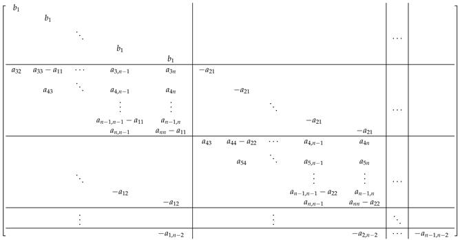
M \in R^{p \times p}

is a matrix which is determined according to (8) from the entries of

A^{c}

and

B^{c}

It is possible to show that the matrix M is determined by

M = M_{1} + M_{2},

where

\begin{matrix} M_{1} & = & Ω (C \otimes A^{c}) Ω^{T} \in R^{p \times p}, \end{matrix}

(12)

\begin{matrix} M_{2} & = & Ω ({[B^{c}, - {A^{c}}_{1 : n, 1 : n - 1}]}^{T} \otimes I_{n}) Ω^{T} \in R^{p \times p}, \end{matrix}

(13)

C = [\begin{matrix} 0 \\ 1 & 0 \\ 1 & ⋱ \\ ⋱ & 0 \\ 1 \end{matrix}],

and

\begin{matrix} Ω & : = & [diag (Ω_{1}, Ω_{2}, \dots, Ω_{n - 1}), 0_{p \times n}] \in R^{p \times n^{2}}, \\ Ω_{k} & : = & [0_{(n - k) \times k}, I_{n - k}] \in R^{(n - k) \times n}, k = 1, 2, \dots, n - 1 . \end{matrix}

(14)

The lower triangular matrix M is nonsingular, since due to the controllability of the system the diagonal entries

b_{1}, a_{21}, \dots a_{n, n - 1}

are different from zero. With the decreasing of the magnitude of these entries, the distance to uncontrollable system decreases and the matrix M becomes worse conditioned. If some or several diagonal elements become zeros, than the system becomes uncontrollable and the matrix M becomes singular. This shows that there is a close connection between the singular values of M and the distance to uncontrollable system. More specifically, for small perturbations

δ A

and

δ B

, the smallest singular value of M can be considered as a measure of the distance to an uncontrollable system.

Since

{∥ h ∥}_{2} \leq \sqrt{{∥ δ A ∥}_{F}^{2} + {∥ δ B ∥}_{F}^{2}}

, we have that

| x_{ℓ} | ⪯ x_{ℓ}^{l i n}, ℓ = 1, 2, \dots, p,

where

x_{ℓ}^{l i n} = {∥ M_{ℓ, 1 : p}^{- 1} ∥}_{2} \sqrt{{∥ δ A ∥}_{F}^{2} + {∥ δ B ∥}_{F}^{2}}

(15)

is the asymptotic (linear) bound on

| x_{ℓ} |

According to (5), the matrix

| δ W |

can be estimated as

| δ W | ⪯ δ W^{l i n} + Δ^{W},

(16)

where

δ W^{l i n} = [\begin{matrix} 0 & x_{1}^{l i n} & x_{2}^{l i n} & \dots & x_{n - 1}^{l i n} \\ x_{1}^{l i n} & 0 & x_{n}^{l i n} & \dots & x_{2 n - 3}^{l i n} \\ x_{2} & x_{n}^{l i n} & 0 & \dots & x_{3 n - 6}^{l i n} \\ ⋮ & ⋮ & ⋮ & ⋱ & ⋮ \\ x_{n - 1^{l i n}} & x_{2 n - 3}^{l i n} & x_{3 n - 6}^{l i n} & \dots & 0 \end{matrix}] \in R^{n \times n}

is a first-order approximation of

| δ W |

and

Δ^{W}

contains higher order terms in x. Thus, an asymptotic (linear) approximation of the matrix

| δ U |

can be determined as

| δ U | ⪯ δ U^{l i n} = | U | | U^{H} δ U | = | U | δ W^{l i n} .

(17)

Consider the sensitivity of a controllable subspace

X = R (U_{X})

of dimension k. Since

{\tilde{U}}_{X} = U_{X} + δ U_{X}, {U_{X}^{p e r p}}^{T} U_{X} = 0,

we have that

sin (Θ_{max} (\tilde{X}, X)) = ∥ {U_{X}^{p e r p}}^{T} {\tilde{U}}_{X} ∥_{2} = ∥ {U_{X}^{p e r p}}^{T} δ U_{X} ∥_{2} = {∥ δ W_{k + 1 : n, 1 : k} ∥}_{2} .

(18)

Equation (18) shows that the sensitivity of the controllable subspace

X

of dimension k is connected to the values of the perturbation parameters

x_{ℓ} = U_{i}^{T} δ U_{j}, ℓ = i + (j - 1) n - \frac{j (j + 1)}{2}, i > k, j = 1, 2, \dots, k

. Consequently, if the perturbation parameters are known, it is possible to find at once sensitivity estimates for all controllable subspaces with dimension

k = 1, 2, \dots, n - 1

. More specifically, let

δ W = [\begin{matrix} * & * & * & \dots & * \\ x_{1} & * & * & \dots & * \\ x_{2} & x_{n} & * & \dots \\ ⋮ & ⋮ & ⋮ & ⋱ & ⋮ \\ x_{n - 1} & x_{2 n - 3} & x_{3 n - 6} & \dots & * \end{matrix}],

where * is an unspecified entry. Then we have that the maximum angle between the perturbed and unperturbed invariant subspace of dimension k is given by

Θ_{max} (\tilde{X}, X) = arcsin (∥ δ W_{k + 1 : n, 1 : k} ∥_{2}) .

(19)

Thus, we obtain the following result.

Theorem 1.

Let the system (1) be reduced into orthogonal canonical form (2) and assume that the Frobenius norms of the perturbations

δ A

and

δ B

are known. Set

L = [\begin{matrix} * & * & * & \dots & * \\ M_{1, 1 : p}^{- 1} & * & * & \dots & * \\ M_{2, 1 : p}^{- 1} & M_{n, 1 : p}^{- 1} & * & \dots & * \\ ⋮ & ⋮ & ⋮ & ⋱ & ⋮ \\ M_{n - 1, 1 : p}^{- 1} & M_{2 n - 3, 1 : p}^{- 1} & M_{3 n - 6, 1 : p}^{- 1} & \dots & * \end{matrix}] \in R^{n \times n . p},

where the matrix M is determined as in (11). Then for the kth controllable subspace of (1), the following asymptotic perturbation bound holds,

Θ_{max}^{l i n} (\tilde{X}, X) \leq arcsin (∥ L_{k + 1 : n, 1 : k p} ∥_{2} {∥ h ∥}_{2}) \leq arcsin (∥ L_{k + 1 : n, 1 : k p} ∥_{2} ∥ \sqrt{{δ A ∥}_{F}^{2} + {∥ δ B ∥}_{F}^{2}}) .

(20)

The proof of Theorem 1 follows directly from (19), replacing the matrix

δ W

by its linear approximation

δ W^{l i n}

and substituting each

x_{ℓ}^{l i n}

by its approximation (15). Note that, as always in the case of perturbation bounds, the equality can be achieved only for specially constructed perturbation matrices

δ A

and

δ B

Similarly to the componentwise sensitivity analysis of the orthogonal transformation matrix, it is possible to find perturbation bounds on the entries of the matrices

A^{c}

and

B^{c}

3. Probabilistic Perturbation Bounds for Controllable Subspaces

3.1. Probabilistic Bounds for Random Matrices

The asymptotic perturbation bounds for controllability subspaces are usually pessimistic especially for high order systems. The conservatism of these estimates can be substantially reduced, if instead of the quantities

{∥ δ A ∥}_{F}

and

{∥ δ B ∥}_{F}

, producing the maximum possible (and unrealistic) perturbation bound (20), we use their estimates obtained for a specified probability. This can be achieved by exploiting the properties of perturbation matrices with random entries. We note that our approach to the analysis of the random matrices is different from the methods proposed by Edelman and Rao [4] and Stewart [21].

Assume we are given an

n \times m

random matrix

δ A

with uncorrelated elements. To bound the entries of this matrix in the perturbation analysis, we have to use the matrix bound

Δ A = [Δ a_{i j}], Δ a_{i j} > 0

, so that

| δ A | ⪯ Δ A

, i.e.,

| δ a_{i j} | \leq Δ a_{i j}, i = 1, 2, \dots, n, j = 1, 2, \dots, m,

(21)

where

Δ a_{i j} = ∥ δ A ∥

and

∥ . ∥

is some matrix norm. If we use the Frobenius norm of

δ A

, we have the deterministic bound

Δ a_{i j} = {∥ δ A ∥}_{F}

that guarantees the fulfillment of (21). However, for such a bound we have that

{∥ Δ A ∥}_{F} = \sqrt{m n} {∥ δ A ∥}_{F},

which yields very pessimistic results for large n and m. That is why to decrease

{∥ Δ A ∥}_{F}

, we shall reduce the entries of

Δ A

, taking a bound with

Δ a_{i j} = {∥ δ A ∥}_{F} / Ξ

, where

Ξ > 1

. Obviously, in the general case such a bound may not satisfy (21) for all i and j. However, we can allow to exist some entries

δ a_{i j}

of the perturbation

δ A

that exceed in magnitude with some prescribed probability the corresponding bound

Δ a_{i j}

. The probability that

| δ a_{i j} | > Δ a_{i j}

can be determined by the Markoff inequality [17]

P {ξ \geq a} \leq \frac{E {ξ}}{a},

(22)

where

P {ξ \geq a}

is the probability that the random variable

ξ

is greater or equal to a given number a and

E {ξ}

is the average (mean value) of

ξ

. We note that the Markoff inequality is valid for arbitrary distribution of

ξ

, which makes it conservative for a specific probability distribution. Applying the Markoff inequality with

ξ

equal to the entry

| δ a_{i j} |

and a equal to the corresponding bound

Δ a_{i j}

, we obtain the following result [19].

Theorem 2.

For an

n \times m

random perturbation

δ A

and a desired probability

0 < P^{r e f} < 1

, the estimate

Δ A = [Δ a_{i j}]

, where

Δ a_{i j} = \frac{{∥ δ A ∥}_{F}}{Ξ},

and

Ξ = (1 - P^{r e f}) \sqrt{m n},

(23)

satisfies the inequality

P {| δ a_{i j} | < Δ a_{i j}} \geq P^{r e f}, i = 1, 2, \dots, n, j = 1, 2, \dots, m .

According to Theorem 2, the using of the scaling factor (23) guarantees that the inequality

| δ a_{i j} | < Δ a_{i j}

holds for each i and j with probability no less than

P^{r e f}

Theorem 2 can be used to decrease the mean value of the bound

Δ A

and hence the magnitude of its entries by the quantity

Ξ

, choosing the desired probability

P^{r e f}

less than 1. The value

P^{r e f} = 1

corresponds to the case of the deterministic bound

Δ A

which fulfills (21). The value

P^{r e f} < 1

corresponds to

Δ a_{i j} = {∥ δ A ∥}_{F} / Ξ

, where

Ξ > 1

. We note that the probability bound produced by the Markoff inequality is very conservative and the actual results are much better than the results predicted by the probability

P^{r e f}

In the perturbation analysis, we frequently encounter the problem of determining a bound on the elements of the vector

x = M f,

(24)

where M is given matrix and

f \in R^{p}

is a random vector with known probabilistic bound on its elements. It may be shown that it is valid the following deterministic linear componentwise bound

| x_{ℓ} | \leq x_{ℓ}^{l i n} : = ∥ M_{ℓ, 1 : p} ∥_{2} {∥ f ∥}_{2}, ℓ = 1, 2, \dots, p .

(25)

A probability bound on

| x_{ℓ} |, ℓ = 1, 2, \dots, p

can be determined by the following theorem [19].

Theorem 3.

If the estimate of the parameter vector x is chosen as

x^{e s t} = | M f | / Ξ

, where Ξ is determined according to

Ξ = \sqrt{p} (1 - P^{r e f}),

(26)

then

P {| x_{ℓ} | \leq ∥ x^{e s t} ∥_{2}} \leq P^{r e f} .

(27)

Since

∥ x^{e s t} ∥_{2} \leq {∥ M ∥}_{2} {∥ f ∥}_{2} / Ξ,

the inequality (27) shows that the probability estimate of the component

| x_{ℓ} |

can be determined, if in the linear estimate (25) we replace the perturbation norm

{∥ f ∥}_{2}

by the probability estimate

{∥ f ∥}_{2} / Ξ

, where the scaling factor

Ξ

is taken as in (26) for a specified probability

P^{r e f}

. In this way, instead of the linear estimate

x_{ℓ}^{l i n}

, we obtain the probabilistic estimate

x_{ℓ}^{e s t} = x_{ℓ}^{l i n} / Ξ = ∥ M_{ℓ, 1 : p} ∥_{2} {∥ f ∥}_{2} / Ξ, ℓ = 1, 2, \dots, p .

3.2. Probabilistic Sensitivity Analysis of Controllable Subspaces

To determine tighter perturbation bounds of the controllable subspaces, we replace the Frobenius norms of the matrix perturbations

δ A

and

δ B

in the linear estimate (20) by much smaller probabilistic estimates of the perturbations entries, determined by using Theorems 2 and 3. This makes possible to decrease with a specified probability the perturbation bounds for the different subspaces achieving realistic results for higher dimensional problems. For this aim, we replace

∥ δ A ∥

and

{∥ δ B ∥}_{F}

in (20) by the ratios

∥ δ A ∥ / Ξ_{A}

and

∥ δ B ∥ / Ξ_{B}

, where

Ξ_{A} = n (1 - P^{r e f}), Ξ_{B} = \sqrt{n} (1 - P^{r e f}) .

Using Theorem 3, the probabilistic perturbation bounds of x and

δ U

can be found from (15) and (17), replacing in (15) the perturbation norms

{∥ δ A ∥}_{F}

and

{∥ δ B ∥}_{F}

by the quantities

{∥ δ A ∥}_{F} / Ξ_{A}

and

∥ δ B ∥ / Ξ_{B}

, respectively. In this way, we obtain the probabilistic asymptotic estimate

Θ_{max}^{e s t} (\tilde{X}, X) = arcsin (∥ L_{k + 1 : n, 1 : k p} ∥_{2} {∥ δ A ∥}_{F} / Ξ)

(28)

of the maximum angle between the perturbed and unperturbed invariant subspace of dimension k.

3.3. A Numerical Example

In this example, we present the asymptotic deterministic perturbation bounds for the controllable subspaces, along with the probabilistic bounds obtained by using the Markoff inequality.

Example 1.

Consider a single-input linear system with matrix A, taken as

A = Q_{0} A_{0} Q_{0}^{- 1}, B = Q_{0} B_{0},

where

\begin{matrix} A_{0} & = & [\begin{matrix} p & 2 p & 3 p & 4 p & \dots & (n - 1) p & n p \\ 5.0 & (n + 1) p & (n + 2) p & (n + 3) p & \dots & (2 n - 2) p & (2 n - 1) p \\ 5.0 & 2 n p & (2 n + 1) p & \dots & (3 n - 4) p & (3 n - 3) p \\ 5.0 & (3 n - 1) p & \dots & (4 n - 6) p & (4 n - 6) p \\ 5.0 & \dots & ⋮ & ⋮ \\ ⋱ & ((n^{2} + n) / 2 - 2) p & ((n^{2} + n) / 2 - 1) p \\ 5.0 & ((n^{2} + n) / 2) p \end{matrix}], \\ p & = & 0.00001 \\ B_{0} & = & {[\begin{matrix} 1 & 0 & 0 & 0 & \dots & 0 & 0 \end{matrix}]}^{T}, \end{matrix}

and the matrix

Q_{0}

is constructed as [1]

\begin{matrix} Q_{0} & = & H_{2} Σ H_{1}, Q_{0}^{- 1} = H_{1} Σ^{- 1} H_{2}, \\ H_{1} & = & I_{n} - 2 u u^{T} / n, H_{2} = I_{n} - 2 v v^{T} / n, \\ u & = & {[1, 1, 1, \dots, 1]}^{T}, v = {[1, - 1, 1, \dots, {(- 1)}^{n - 1}]}^{T}, \\ Σ & = & diag (1, σ, σ^{2}, \dots, σ^{n - 1}), \end{matrix}

where

H_{1}, H_{2}

are elementary reflections, σ is taken equal to

1.01

and

cond (Q_{0}) = 2.678

. The parameter σ is used to change the conditioning of the matrix

Q_{0}

and the parameter p is used to change the conditioning of the controllable subspaces.

The perturbation of A and B are taken as

δ A = 10^{- 8} A_{r}

δ B = 10^{- 8} B_{r}

, where

A_{r}

and

B_{r}

are matrices with random entries with normal distribution and

{∥ δ A ∥}_{F} = 9.91429 \times 10^{- 7}

{∥ δ B ∥}_{F} = 9.50807 \times 10^{- 8}

. The matrix M in (11) is of order

p = 4950

and its inverse satisfies

∥ M^{- 1} ∥_{2} = 1.88694 \times 10^{4}

. This shows that the problem for the sensitivity of the controllable subspaces is ill-conditioned since the perturbations of A and B can be magnified

10^{4}

times in x and, consequently, in

δ U

and

Θ (\tilde{X}, X)

. The minimum singular value of M is equal to

5.29957 \times 10^{- 5}

, which shows that perturbations of size

10^{- 5}

may transform the given system to uncontrollable one.

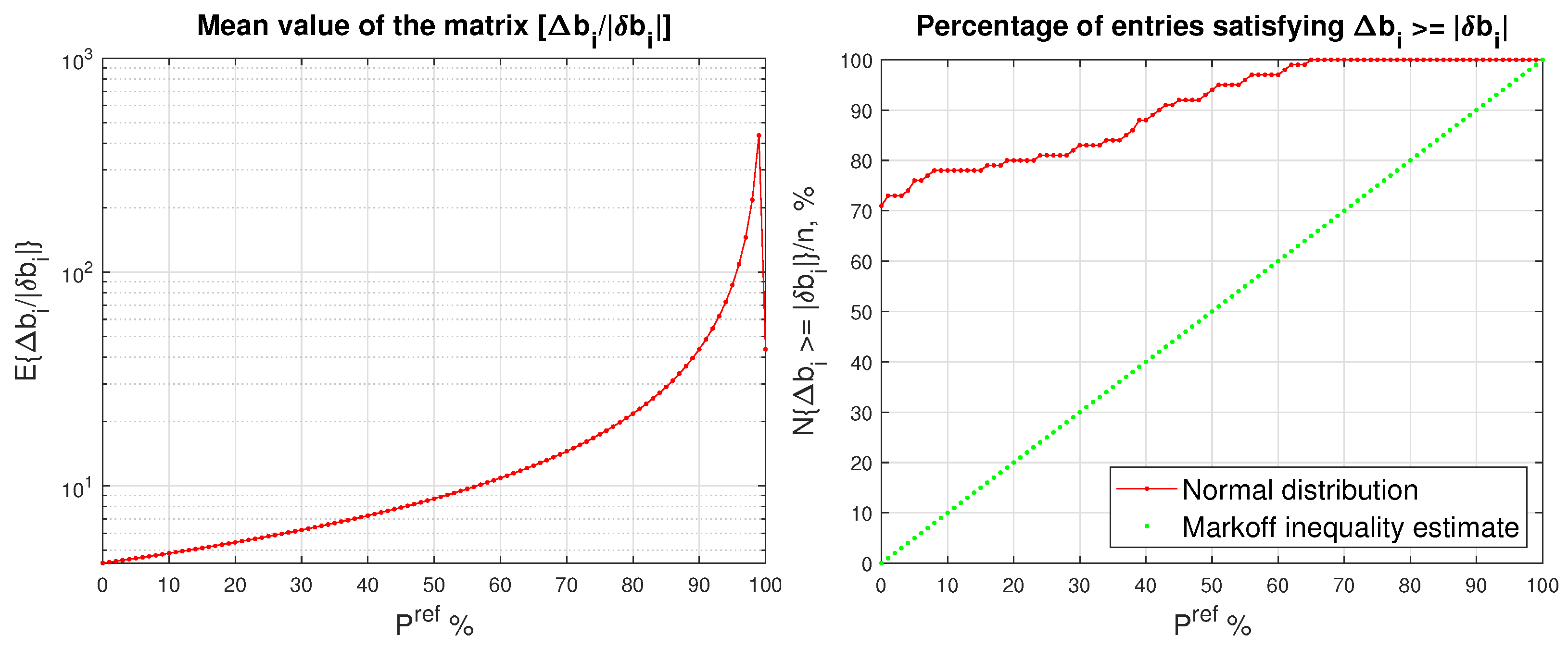
In Figure 1 we show the mean value of the matrix

[Δ a_{i j} / | δ a_{i j} |]

and the relative number

N {Δ a_{i j} \geq | δ a_{i j} |} / (n^{2})

of the entries of the matrix

| δ A |

for which

| δ a_{i j} | \leq | Δ a_{i j} |

, and in Figure 2 - the corresponding quantities for

| δ B |

, obtained for normal distribution of the entries of

δ A

and

δ B

and for different values of the desired probability

P^{r e f}

. For the case of

P^{r e f} = 90 %

, the size of the probability entry bound

Δ a_{i j}

decreases 10 times in comparison with the size of the entry bound

{∥ δ A ∥}_{F}

, which allows to decrease the mean value of the ratio

Δ a_{i j} / | δ a_{i j} |

from

840.86

84.086

(Table 1). For

P^{r e f} = 40 %

, the probability bound

Δ a_{i j}

is 60 times smaller than the bound

{∥ δ A ∥}_{F}

and even for this small desired probability the number of entries for which

| δ a_{i j} | \leq | Δ a_{i j} |

is still

90.34 %

. The corresponding quantities for

δ B

are shown in Table 2.

Table 1. The mean value of the ratios

[Δ a_{i j} / | δ a_{i j} |]

and the relative number of entries for which

N {Δ a_{i j} > | δ a_{i j} |} / n^{2}

, obtained for different values of

P^{r e f}

n = 100

Table 1. The mean value of the ratios

[Δ a_{i j} / | δ a_{i j} |]

and the relative number of entries for which

N {Δ a_{i j} > | δ a_{i j} |} / n^{2}

, obtained for different values of

P^{r e f}

n = 100

$P^{r e f}$	$Ξ$	$E {[Δ a_{i j} / \| δ a_{i j} \|]}$	$N {Δ a_{i j} > \| δ a_{i j} \|} / n^{2}$
%			%
$100.0$	$1.0000 \times 10^{0}$	$8.4086 \times 10^{2}$	$100.0000$
$90.0$	$1.0000 \times 10^{1}$	$8.4086 \times 10^{1}$	$100.0000$
$80.0$	$2.0000 \times 10^{1}$	$4.2043 \times 10^{1}$	$100.0000$
$70.0$	$3.0000 \times 10^{1}$	$2.8029 \times 10^{1}$	$99.8800$
$60.0$	$4.0000 \times 10^{1}$	$2.1022 \times 10^{1}$	$98.8200$
$50.0$	$5.0000 \times 10^{1}$	$1.6817 \times 10^{1}$	$98.8200$
$40.0$	$6.0000 \times 10^{1}$	$1.4014 \times 10^{1}$	$90.3400$

Table 2. The mean value of the ratios

[Δ b_{i j} / | δ b_{i j} |]

and the relative number of entries for which

N {Δ b_{i j} > | δ b_{i j} |} / n

, obtained for different values of

P^{r e f}

n = 100

Table 2. The mean value of the ratios

[Δ b_{i j} / | δ b_{i j} |]

and the relative number of entries for which

N {Δ b_{i j} > | δ b_{i j} |} / n

, obtained for different values of

P^{r e f}

n = 100

$P^{r e f}$	$Ξ$	$E {[Δ b_{i j} / \| δ b_{i j} \|]}$	$N {Δ b_{i j} > \| δ b_{i j} \|} / n^{2}$
%			%
$100.0$	$1.0000 \times 10^{0}$	$4.3503 \times 10^{1}$	$100.0000$
$90.0$	$1.0000 \times 10^{0}$	$4.3503 \times 10^{1}$	$100.0000$
$80.0$	$2.0000 \times 10^{0}$	$2.1751 \times 10^{1}$	$100.0000$
$70.0$	$3.0000 \times 10^{0}$	$1.4501 \times 10^{1}$	$100.0000$
$60.0$	$4.0000 \times 10^{0}$	$1.0876 \times 10^{1}$	$97.0000$
$50.0$	$5.0000 \times 10^{0}$	$8.7005 \times 10^{0}$	$94.0000$
$40.0$	$6.0000 \times 10^{0}$	$7.2504 \times 10^{0}$	$88.0000$

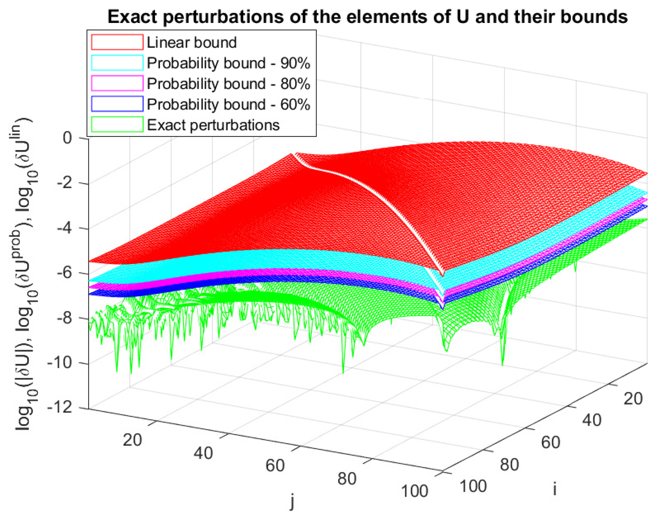
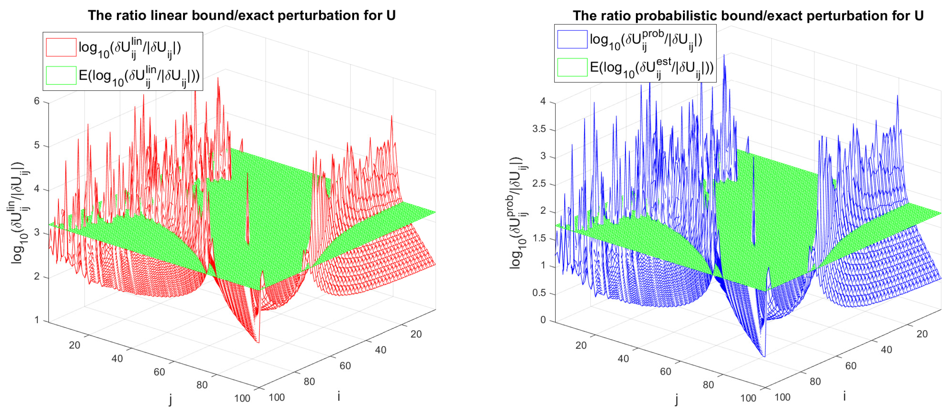
In Figure 3 we compare the asymptotic bound

δ U^{l i n}

and the probabilistic estimate

δ U^{p r o b}

with the actual componentwise perturbations

| δ U |

for normal distribution of perturbation entries and probabilities

P^{r e f} = 90 %, 80 %

and

60 %

. The probabilistic bound

δ U^{p r o b}

is much tighter than the linear bound

δ U^{l i n}

and the inequality

| δ U | ⪯ δ U^{p r o b}

is satisfied for all entries and chosen probabilities. In particular, the size of the estimate

δ U^{p r o b}

is 10 times smaller than the linear estimate

δ U^{l i n}

for

P^{r e f} = 90 %

, 20 times for

P^{r e f} = 80 %

and 40 times for

P^{r e f} = 60 %

. In Figure 4 we show the ratio

[δ U_{i j}^{l i n} / | δ U_{i j} |]

(left) and the ratio

[δ U_{i j}^{p r o b} / | δ U_{i j} |]

(right) for

P^{r e f} = 0.6

for normal random distributions of the entries of the matrices A and B. Note that the mean value of ratio for the probabilistic estimate is 40 times smaller than the mean value for the deterministic estimate and its value for each i and j is greater than 1.

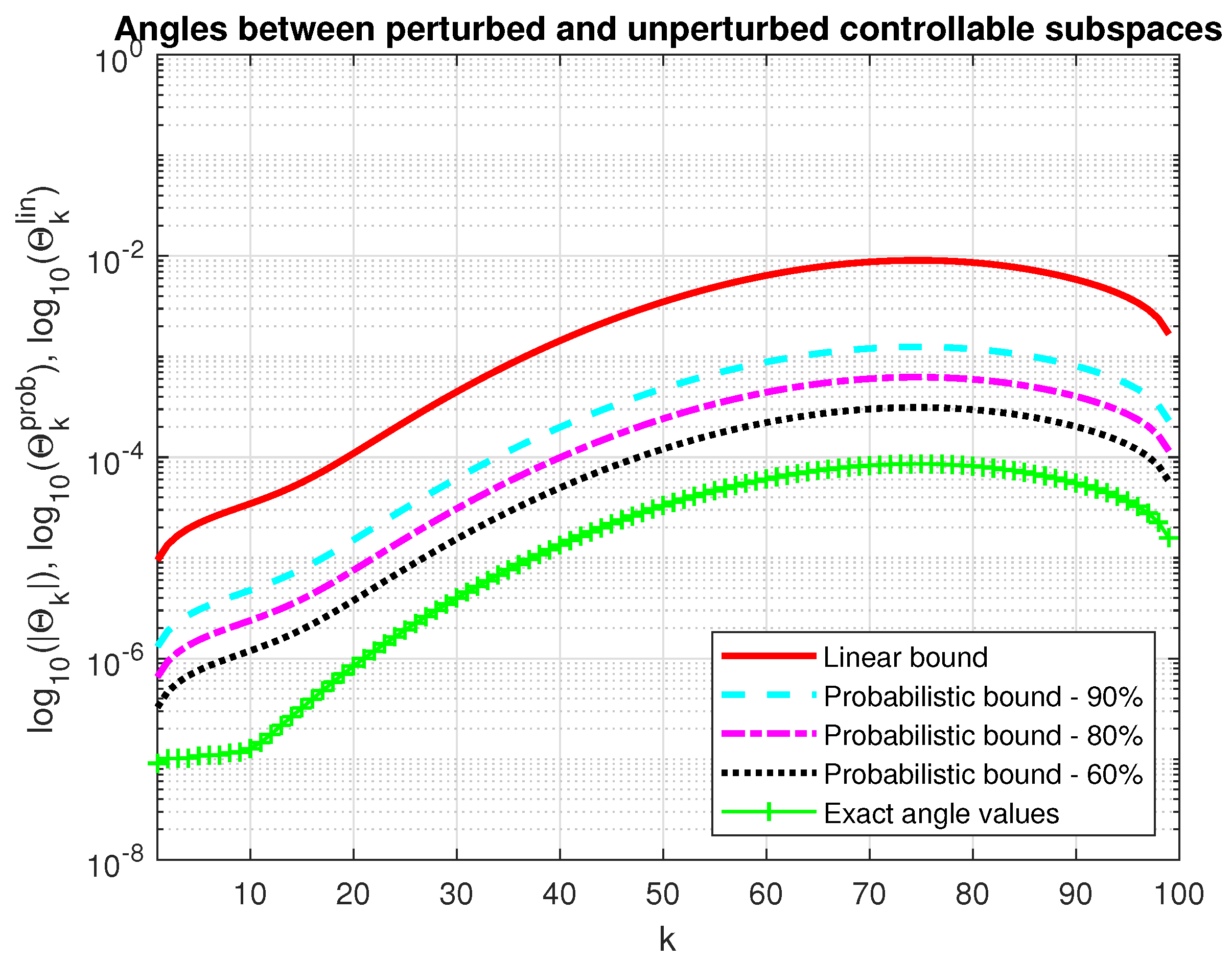
In Figure 5 we show the asymptotic bound

δ Θ_{k}^{l i n}

and the probabilistic estimate

δ Θ_{k}^{p r o b}

along with the exact value

| δ Θ_{k} |

of the maximum angle between the perturbed and unperturbed controllable subspace of dimension

k = 1, 2, \dots, n - 1

for the same probabilities

P^{r e f} = 90 %, 80 %

and

60 %

. The probability estimate satisfies

| δ Θ_{k} | < δ Θ_{k}^{e s t}

for all

1 \leq k < 100

4. Conclusions

In this paper we present asymptotic and probabilistic perturbation bounds of the controllable subspaces of linear single-input control systems. The probabilistic bounds are considerably less conservative than the corresponding deterministic bounds with sufficiently high probability that make them suitable for high order problems. However, they may require a large number of computation due to the using of the Kronecker products. The analysis presented in this paper, is also valid for linear discrete-time single-input systems with a state-space description

x_{k + 1} = A x_{k} + B u_{k} .

By duality, the results of this paper can be also used to analyze the observability subspaces of linear systems.

Funding

This research received no external funding.

Institutional Review Board Statement

Not applicable.

Informed Consent Statement

Not applicable.

Data Availability Statement

The datasets generated during the current study are available from the author upon reasonable request.

Conflicts of Interest

The author declares that the research was conducted in the absence of any commercial or financial relationships that could be construed as a potential conflict of interest.

Notation

$R$ ,	the set of real numbers;
$R^{n \times m}$ ,	the space of $n \times m$ real matrices;
$A = [a_{i j}]$ ,	a matrix with entries $a_{i j}$ ;
$A_{j}$ ,	the jth column of A;
$A_{i, 1 : n}$ ,	the ith row of an $m \times n$ matrix A;
$A_{i_{1} : i_{2}, j_{1} : j_{2}}$ ,	the part of matrix A from row $i_{1}$
	to $i_{2}$ and from column $j_{1}$ to $j_{2}$ ;
$Low (A)$ ,	the strictly lower triangular part of A;
$\| A \|$ ,	the matrix of absolute values of the elements of A;
$A^{T}$ ,	the transposed of A;
$A^{- 1}$ ,	the inverse of A;
$0_{m \times n}$ ,	the zero $m \times n$ matrix;
$I_{n}$ ,	the unit $n \times n$ matrix;
$δ A$ ,	the perturbation of A;
${∥ A ∥}_{F}$ ,	the Frobenius norm of A;
$: =$ ,	equal by definition;
⪯,	relation of partial order. If $a, b \in R^{n}$ , then $a ⪯ b$ means
	$a_{i} \leq b_{i}, i = 1, 2, \dots, n$ ;
$X = R (X)$ ,	the subspace spanned by the columns of X;
$U^{⊥}$ ,	the orthogonal complement of U, $U^{H} U^{⊥} = 0$ ;
$A \otimes B$ ,	the Kronecker product of A and B;
$P {y > y}$ ,	the probability of the event ${y > y}$ ;
$E {ξ}$ ,	the average value or mean of the random variable $ξ$ ;
$N {a_{i j} \geq b_{i j}}$ ,	the number of the entries of A that are
	greater or equal to the corresponding entries of B.

References

C. A. Bavely and G. W. Stewart, An algorithm for computing reducing subspaces by block diagonalization, SIAM J. Numer. Anal., 16 (1979), pp. 359–367. [CrossRef]
D. Boley and W.-S. Lu, Measuring how far a controllable system is from an uncontrollable one, IEEE Trans. Automat. Control, 31(1986), 249–251. [CrossRef]
J.W. Demmel, On Condition Numbers and the Distance to the Nearest Ill-Posed Problem, Numer. Math., 51(1987), 251–289. [CrossRef]
A. Edelman and N.R. Rao, Random matrix theory, Acta Numer., 14 (2005), pp. 1–65. [CrossRef]
R. Eising, Between controllable and uncontrollable, Systems & Control Letters, 4 (1984), 263–264. [CrossRef]
G. H. Golub and C. F. Van Loan, Matrix Computations, The Johns Hopkins University Press, Baltimore, MD, fourth ed., 2013. ISBN 978-1-4214-0794-4.
J. P. Hespanha, Linear Systems Theory, Princeton University Press, Priceton, NJ, second ed. 2018. ISBN 978-0691179575.
S. C. Johnson and M. Wicks and M. Žefran and R. A. DeCarlo, The Structured Distance to the Nearest System Without Property P, IEEE Trans. Automat. Control, 63 (2018), 2960–2975. [CrossRef]
M. Konstantinov and P. Petkov, Perturbation Methods in Matrix Analysis and Control, NOVA Science Publishers, Inc., New York, 2020, https://novapublishers.com/shop/perturbation-methods-in-matrix-analysis-and-control.
M. Konstantinov, P. Petkov, N. Christov, Invariants and canonical forms for linear multivariable systems under the action of orthogonal transformation groups, Kybernetika, 17 (1981), 5, 413-424. ISSN 0024-5954.
M. Konstantinov, P. Petkov, N. Christov, Orthogonal invariants and canonical forms for linear controllable systems, IFAC Proceedings Volumes, 14 (1981), 49 -– 54. [CrossRef]
M. Konstantinov, P. Petkov, D. Gu., I. Postlethwaite, Perturbation analysis of orthogonal canonical forms, Linear Algebra Appl., 251 (1997), 267-291. [CrossRef]
A. J. Laub and A. Linnemann, Hessenberg and Hessenberg/triangular forms in linear system theory, Int. J. Control, 44(1986), 1523–1547. [CrossRef]
The MathWorks, Inc., MATLAB Version 9.9.0.1538559 (R2020b), Natick, MA, 2020, http://www.mathworks.com.
E. Mengi, On the estimation of the distance to uncontrollability for higher order systems, SIAM J. Matrix Anal. Appl., 30(2008), 154–172. [CrossRef]
C. Paige, Properties of numerical algorithms related to computing controllability, IEEE Trans. Automat. Control, 26 (1981), 130–138. [CrossRef]
A. Papoulis, Probability, Random Variables and Stochastic Processes, McGraw Hill, Inc., New York, 3rd edition, 1991. ISBN 0-07-048477-5.
P. Petkov, Perturbation bounds for orthogonal canonical forms and numerical controllability analysis, IEEE Trans. Automat. Control, 38 (1993), 639-643. [CrossRef]
P. Petkov, Probabilistic Perturbation Bounds of Matrix Decompositions, Numer. Linear Algebra Appl., 31(2024), 1–40. [CrossRef]
P. Petkov, Probabilistic Perturbation Bounds for Invariant, Deflating and Singular Subspaces, Axioms, 13(2024), 597. [CrossRef]
G. W. Stewart, Stochastic perturbation theory, SIAM Rev., 32 (1990), pp. 579–610. [CrossRef]
G. W. Stewart, Matrix Algorithms; Vol. II: Eigensystems, SIAM: Philadelphia, PA, 2001. ISBN 0-89871-503-2.
G. W. Stewart and J.-G. Sun, Matrix Perturbation Theory, Academic Press, New York, 1990. ISBN 978-0126702309.
P. M. Van Dooren, The generalized eigenstructure problem in linear system theory, IEEE Trans. Automar. Contr., 26 (1981), pp. 111-129. [CrossRef]
M. Wicks, R. A. DeCarlo. Computing the distance to an uncontrollable system, IEEE Trans. Automat. Control, 36 (1991), 39–49. [CrossRef]
W. M. Wonham, Linear Multivariable Control. A Geometric Approach, 3rd ed., Springer-Verlag, New York, 1985. ISBN 0-387-96071-6.
Z. Yun and Y. Chengwu, Formulae for the distance between controllable and uncontrollable linear systems, Systems & Control Letters, 21(1993), 173–180. [CrossRef]

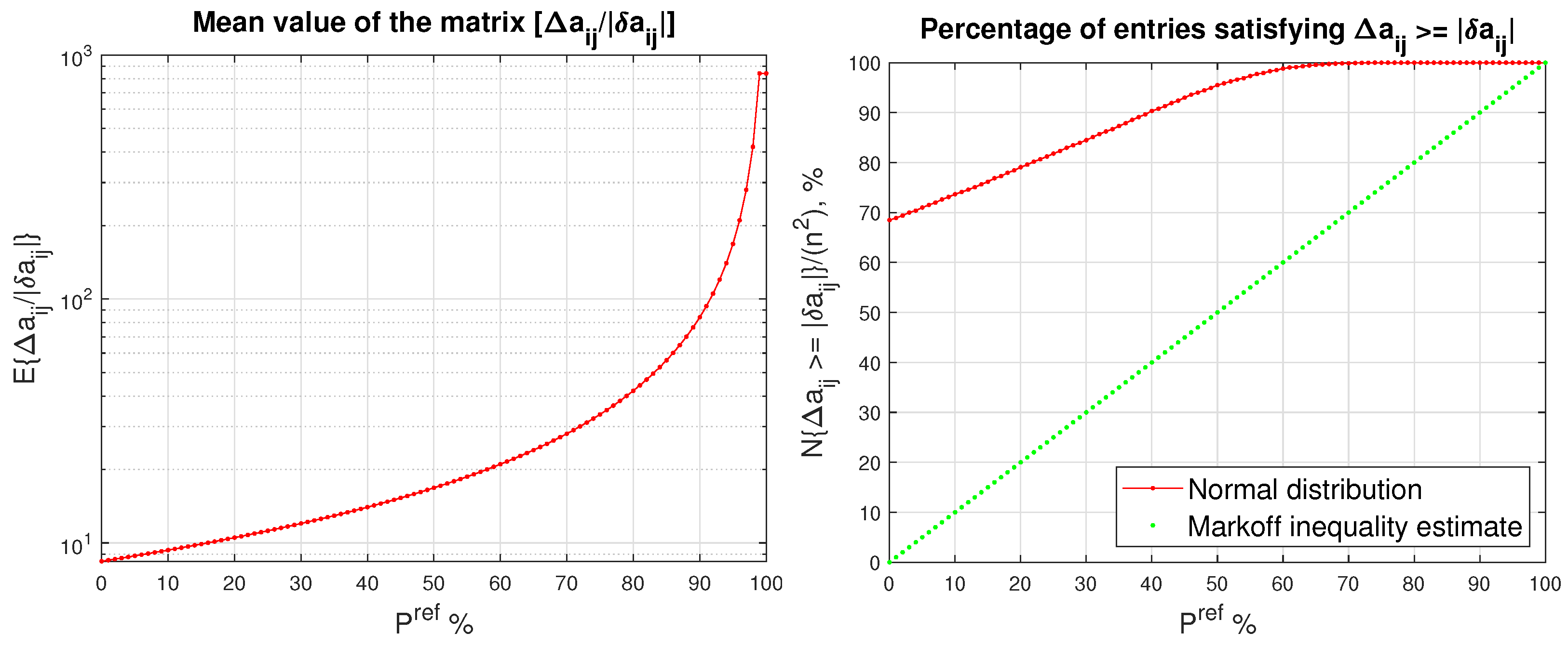
Figure 1. The mean value of

[Δ a_{i j} / | δ a_{i j} |]

as a function of

P^{r e f}

(left) and the mean value of

N {Δ a_{i j} > | δ a_{i j} |} / n^{2}

(right) as a function of

P^{r e f}

for a normal random distributions of the entries of the

100 \times 100

matrix A

Figure 1. The mean value of

[Δ a_{i j} / | δ a_{i j} |]

as a function of

P^{r e f}

(left) and the mean value of

N {Δ a_{i j} > | δ a_{i j} |} / n^{2}

(right) as a function of

P^{r e f}

for a normal random distributions of the entries of the

100 \times 100

matrix A

Figure 2. The mean value of

[Δ b_{i j} / | δ b_{i j} |]

as a function of

P^{r e f}

(left) and the mean value of

N {Δ b_{i j} > | δ b_{i j} |} / n^{2}

(right) as a function of

P^{r e f}

for a normal random distributions of the entries of the

100 \times 1

matrix B

Figure 2. The mean value of

[Δ b_{i j} / | δ b_{i j} |]

as a function of

P^{r e f}

(left) and the mean value of

N {Δ b_{i j} > | δ b_{i j} |} / n^{2}

(right) as a function of

P^{r e f}

for a normal random distributions of the entries of the

100 \times 1

matrix B

Figure 3. Perturbation bounds of the entries of U for different probabilities

Figure 4. The ratio

[δ U_{i j}^{l i n} / | δ U_{i j} |]

(left) and the ratio

[δ U_{i j}^{p r o b} / | δ U_{i j} |]

for

P^{r e f} = 0.6

(right) for normal random distributions of the entries of the matrices A and B

Figure 4. The ratio

[δ U_{i j}^{l i n} / | δ U_{i j} |]

(left) and the ratio

[δ U_{i j}^{p r o b} / | δ U_{i j} |]

for

P^{r e f} = 0.6

(right) for normal random distributions of the entries of the matrices A and B

Figure 5. Angles between the perturbed and unperturbed controllable subspaces and their bounds

Disclaimer/Publisher’s Note: The statements, opinions and data contained in all publications are solely those of the individual author(s) and contributor(s) and not of MDPI and/or the editor(s). MDPI and/or the editor(s) disclaim responsibility for any injury to people or property resulting from any ideas, methods, instructions or products referred to in the content.

© 2024 by the authors. Licensee MDPI, Basel, Switzerland. This article is an open access article distributed under the terms and conditions of the Creative Commons Attribution (CC BY) license (http://creativecommons.org/licenses/by/4.0/).

Copyright: This open access article is published under a Creative Commons CC BY 4.0 license, which permit the free download, distribution, and reuse, provided that the author and preprint are cited in any reuse.

Alerts

MDPI Initiatives

Important Links

Choose an area of interest and we will send you notifications of new preprints at your preferred frequency.

Disclaimer

Asymptotic and Probabilistic Perturbation Analysis of Controllable Subspaces

Abstract

Keywords:

Subject:

1. Introduction

2. Asymptotic Perturbation Bounds for Controllability Subspaces

2.1. Orthonormal Bases of the Controllable Subspaces

2.2. Perturbation Bounds by the Splitting Operator Method

3. Probabilistic Perturbation Bounds for Controllable Subspaces

3.1. Probabilistic Bounds for Random Matrices

3.2. Probabilistic Sensitivity Analysis of Controllable Subspaces

3.3. A Numerical Example

4. Conclusions

Funding

Institutional Review Board Statement

Informed Consent Statement

Data Availability Statement

Conflicts of Interest

Notation

References

MDPI Initiatives

Important Links

Subscribe