Performance Evaluation of Weather@home2 Simulations over West African Region

Weather and climate forecasting is extremely important for improving the socio-economic well-being of the West African region. It safe-guards the region from weather and climate related disasters. Hence, utilization of products from climate models are being encouraged and have therefore become essential tools and life-savers, in spite of the fact that climate models do not fully comply with attributes of forecast qualities - RASAP: reliability, association, skill, accuracy and precision. This paper thus quantitatively evaluates, in comparisons to CRU and ERA5 datasets, the RASAP compliance-level of the weather@home2 modelling system (w@h2: a successor to the well-known weather@home1 modelling system) which now produces an exceptionally large number of ensembles of simulations (>10,000). Having been designed for the investigation of the behavior of extreme weather under anthropogenic climate change, findings show that the performance of w@h2 in terms of climate variability may be more relevant than measures of the mean climatology. To some significant extent w@h2 model provides little, if any, predictive information for precipitation during the dry season, but may provide useful information during the monsoon seasons as well as skill to capture the Little Dry Season over the Guinea zone; predictive skills for the onset season suggest that the model is getting processes right. The w@h2 model is also able to reproduce all the annual characteristics of the surface maximum air temperature over the sub-region with skill to detect heat waves that usually ravage West Africa during the boreal spring. With synchronization > 80% the model has the ability to reliably / accurately simulate the actual anomaly signs of the observed climate parameters which is one of the special attributes of a model that is needed for seasonal climate predictions and applications. The large sample sizes produced by the w@h2 model are able to show that sampling quality of the tails of the distribution is no longer the primary constraint / source of uncertainty. The study further furnishes a prospective user with information on whether the model might be “useful or not” for a particular application.

Keywords:

Subject:

Environmental and Earth Sciences - Atmospheric Science and Meteorology

Supplementary Material

supplementary.xls (28.50KB )

1. Introduction

Over the years, especially in West African region, researchers’ and stakeholders’ confidence in the use of climate models is increasing. This is due to improvements in nearly all aspects of climate models’ fidelity and skill, as well as more detailed understanding of the degree of fidelity and skill (Mariotti et al., 2011; Nikulin et al., 2012; Diallo et al., 2013; Klein et al., 2015; Sylla et al., 2015). Consequently, information from climate models are extensively being used by the region’s policy makers and various socio-economic sectors (e.g., water resources management, agriculture, engineering, environmental management, health, insurance, researchers, etc.) either for risk management or for day-to-day, season-to-season or long-term strategies and planning (Tall et al., 2012; Niang et al., 2014; Nkiaka et al., 2019). Proliferation of climate models calls for caution among researchers and stakeholders. To calm the fears and concerns of prospective users, thorough performance evaluations of climate models have to be carried out before their eventual utilization.

The performance of a climate model can be evaluated according to these five attributes of forecast qualities, hereafter known as RASAP: R (reliability), A (association), S (skill), A (accuracy), and P (precision) (Storch and Zwiers, 2003; Walther and Moore, 2005; Ebert et al., 2013; Wilson and Giles, 2013). In short terms, reliability can be referred to as the ability of a forecast to provide an unbiased estimate. According to Mason (2004) and Ebert et al. (2013) it is a key quality of a probabilistic long-range forecast. Murphy (1988 and 1995) described association as a measure of linear relationship between forecast and observation. Skill is a comparative quantity that shows if a set of forecasts is better than a reference set, e.g., climatology, persistence, etc. It is a measure of relative ability of a set of forecasts with respect to some set of standard reference forecasts (Wilks, 1995; Mason, 2004; Weigel et al., 2006; Kim et al., 2016). Accuracy can be referred to as the overall correspondence or level of agreement between model and observation. According to Wilson and Giles (2013) it summarizes the overall quality of a forecast; while precision, a measure of uncertainty, is simply the absence of random error, i.e., a measure of statistical variance of an estimation that is independent of a true value (Debanne, 2000). Precision is described as the spread of the data whenever sampling is involved (West, 1999).

Climate models do not fully pass thresholds for these measures over many regions of the world, including the West African region, and hence they are not fully RASAP compliant. Assessing their degree of RASAP compliance therefore provides a quantitative evaluation of their ability to represent regional climate. Performances of several climate models have been evaluated over the West African region. While some of these evaluations have been motivated by the importance of the West African monsoon and its circulation features, others have been interested in mechanisms and processes responsible for rainfall regimes (Xue et al., 2010; Nikulin et al., 2012; Diallo et al., 2013). There have also been some evaluations to improve the understanding of the nature of the interactions across the different dynamical systems within the West African monsoon (Mariotti et al., 2011; Zaroug et al., 2013; Diallo et al., 2014; Klein et al., 2015; Sylla et al., 2015).

A major challenge in evaluating RASAP performance is that many of the measures require large initial-condition ensembles of simulations, which can be computationally prohibitive. In this paper we focus on evaluating the RASAP performance of a modelling system that has produced an exceptionally large number of simulations, thus providing material for robust tests against the RASAP measures – the weather@home2 modelling system (hereafter w@h2). w@h2 is a successor to the well-known weather@home modelling system (hereafter w@h1: Massey et al., 2015; Guillod et al., 2017). Generally, the w@h2 modelling system can generate very large ensembles of simulations (>10,000) that allow denser sampling of the climate distributions. This is made possible by the enlistment of thousands of volunteers around the world who, on their personal computers, run simulations starting from different initial conditions. The results are then uploaded onto the climateprediction.net (CPDN: https://www.climateprediction.net) server facility hosted by the University of Oxford (Anderson, 2004). The project runs the Hadley Centre Regional Model version 3P (HadRM3P) nested in the Hadley Centre Global Atmospheric Model (HadAM3P-N96: Jones et al., 2004) over various domains of the world, now including West Africa. Details of the improvements made in w@h2 in comparisons to w@h1 are discussed in Guillod et al. (2017).

The w@h2 modelling system has been designed for the investigation of the behavior of extreme weather under anthropogenic climate change. This means that measures of the performance of the model in terms of climate variability are more relevant than measures of the mean climatology (Bellprat and Doblas-Reyes, 2016; Lott and Stott, 2016; Bellprat et al., 2019). If the w@h2 modelling system is to be used to understand changes in extreme weather over West Africa, then it is pertinent to evaluate the performance of the w@h2 simulations over the region.

Specifically, we are asking the following questions – 1. Are the w@h2 simulations, over West Africa, reliable? 2. Does any linear association exist between the simulations and observations / reanalysis over West Africa? 3. Do these simulations have skill over West Africa? 4. Are the simulations accurate, as well as precise over this region? These questions are asked with a view to understanding whether the w@h2 simulations may be useful for extreme event attribution analysis over West Africa. This paper will utilize a series of statistical metrics to calculate the selected attributes of forecast qualities, i.e., RASAP, to provide insights on the nature of the w@h2 simulations.

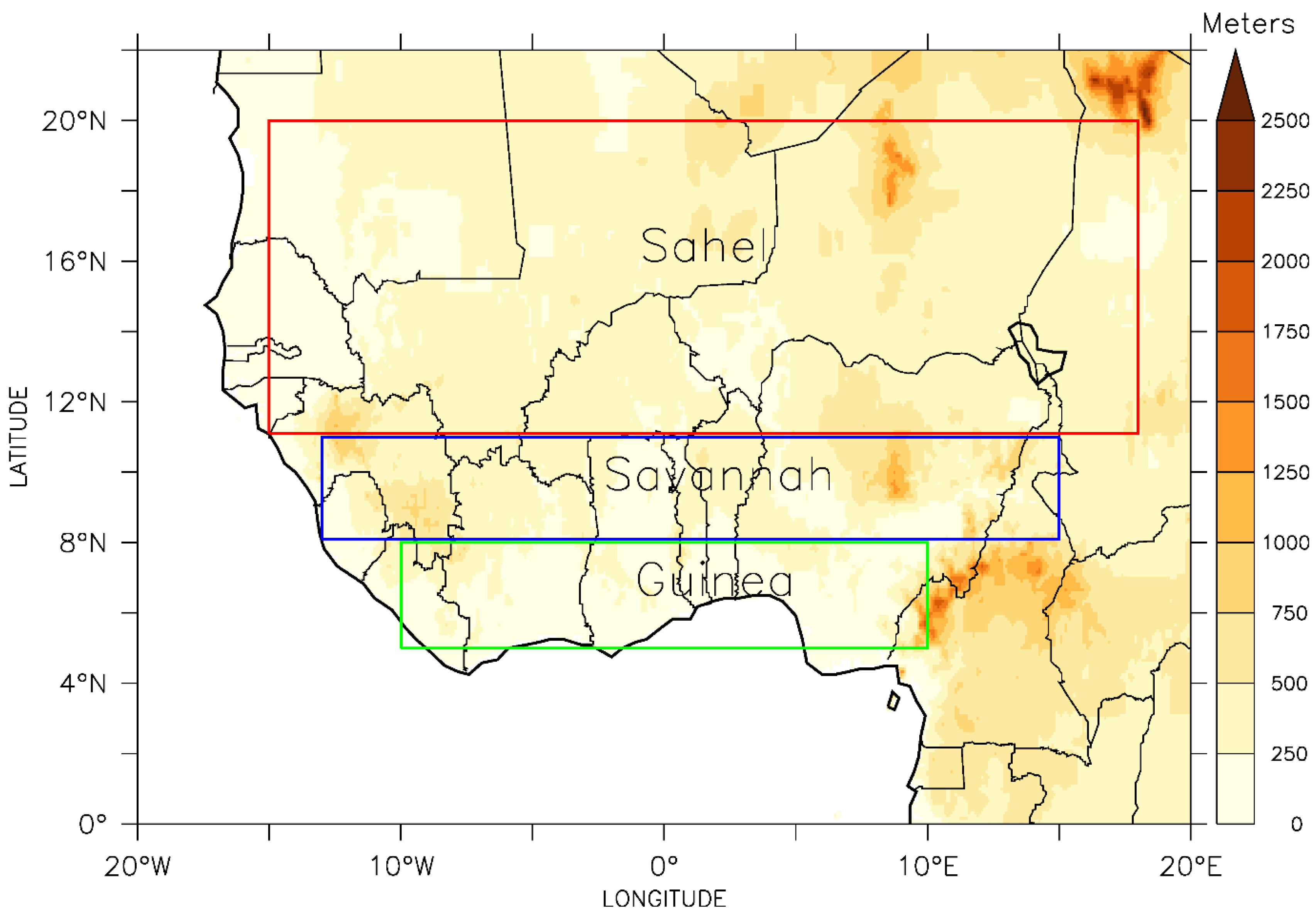
West Africa, a unique region of atmospheric complexities, is a tropical land mass located roughly within longitudes 20^oW to 20^oE, and latitudes 0^o to about 25^oN of the African continent (Figure 1). The region comprises three climatic zones, namely: Guinea – a tropical rain forest along the Atlantic coast; Savannah – a transition zone of short trees and grasses; and the Sahel – an Arid desert in the northern inlands (Nicholson and Palao, 1993; Nicholson, 1995; Omotosho and Abiodun, 2007).

West African climates result from the interactions of two migrating air masses: tropical maritime and tropical continental air masses. At the surface, these two air masses meet at a belt of variable width and stability called the Inter-Tropical Discontinuity (ITD: Omotosho, 2007) or the Inter-Tropical Convergence Zone (ITCZ) if at upper level. The north and south migration of ITD, which follows the annual cycle, influences the climate of the region (Nicholson, 1993; Omotosho, 2007). Besides ITD there are other key climate modification mechanisms over West Africa. Most relevant are the El Niño Southern Oscillation (ENSO; Latif and Grotzner, 2000; Camberlin et al., 2001; Newman et al., 2003), the sea surface temperature (SST) anomalies over the Gulf of Guinea (GOG; Omotosho and Abiodun, 2007; Odekunle and Eludoyin, 2008), the African Easterly Jet (AEJ; Diedhiou et al., 1998; Grist and Nicholson, 2001; Afiesimama, 2007), and the thermal lows (Parker et al., 2005; Lavaysse et al., 2006, 2009, 2010). The region’s climate is classified into two seasons driven by the position of the ITD – the dry season and the rainy season. The period of dry season runs approximately from November to March / April. It is a time of hot and dry tropical continental air mass driven by the ridges from the northern hemispheric mid-latitude high pressure system. During these periods, the prevailing northeasterly winds, north of the ITD, bring dry and dusty conditions across the region with the southernmost extension of this air mass occurring in January between latitudes 5° and 7°N. Tropical maritime southwesterly air mass is found at the southern ends of the ITD. The moist air mass dominates during the periods of the rainy seasons. The region’s rainy seasons run from April / May to October depending on the climatic zone of interest (Figure 1: Nicholson and Grist, 2003; Redelsperger et al., 2006; Omotosho and Abiodun, 2007). The northernmost penetration of the wet air mass is in August, usually between latitudes 19° and 22°N. With all these atmospheric complexities, the use of dynamical climate models for forecasting of weather and projection of climate are indispensable over the region. Therefore, performance evaluation of meteorological forecasts and or simulations is crucial for understanding the errors of, monitoring the accuracy of, and making progress in climate modelling systems (Ebert et al., 2013).

While this section introduces the motivations and concept of the study including the description of the study domain and its complexities, section 2 will discuss the data sets analysed in the paper, and the adopted analysis procedures. Section 3 will describe the results, while Section 4 will provide summary and conclusions.

2. Datasets and the Analysis Procedures

2.1. Datasets – Observation, Reanalysis, and Simulation Data Sets

This study used monthly precipitation and near surface maximum air temperature from three categories of datasets – gridded observational, reanalysis, and w@h2 simulation. The observation datasets are from the University of East Anglia Climate Research Unit (CRU version TS4.03 (CRU-TS4): https://crudata.uea.ac.uk/cru/data/hrg/; New et al., 2000; Harris et al., 2013). This is based on analysis of records of observations from over 4000 weather stations. The reanalysis datasets are from the European Centre for Medium-Range Weather Forecasts (ECMWF – ERA version 5 (ERA5): https://www.ecmwf.int/en/forecasts/datasets/reanalysis-datasets/era5; Hersbach et al., 2018). Simulated datasets are from the w@h2 modelling system obtained from the CPDN team (https://www.climateprediction.net) at the University of Oxford. The w@h2 modelling system (HadRM3P nested in HadAM3P-N96: Jones et al., 2004) is executed in various regional domains over the world, including an African domain that encompasses West Africa.

These datasets have different spatial resolutions. The observed variables (CRU) are on a horizontal grid resolution of 0.5°x0.5° longitude–latitude, while the reanalysis (ERA5) datasets have a horizontal resolution of 30 km grid. Horizontal resolution of w@h2 simulations is about 0.22^o (25 km) compared to about 0.44^o (50 km) in w@h1. For uniformity, the horizontal resolutions of all the simulated (w@h2) and the reanalysis (ERA5) datasets were re-gridded to match that of the observation (CRU) dataset before they were analyzed. All monthly simulated variables from w@h2 used in this study are from 71 ensemble members per year. Each ensemble member differs only slightly in their initial conditions and we focus on the 31-year period from January 1987 to December 2017.

2.2. Methodology and Analysis Procedures

This paper aims to evaluate the performances of the w@h2 simulations over West Africa in line with the qualities of selected forecast attributes – RASAP. In comparisons to CRU and ERA5 datasets, w@h2 simulations are subjected to a series of quantitative statistical metrics to calculate RASAP measures. As depicted in Table 1, temporal and spatial analyses of these statistical metrics are carried out and then presented in various graphical formats for interpretation. We also place some figures in the supplementary domain of this paper for clarity of purpose.

Results and analyses from this study will be presented on the basis of calendar months, in reflection of their common usage in climate services throughout the region and of the typical monthly duration of noteworthy extreme events in the region (e.g., Lawal et al., 2019).

3. Results

3.1. Seasonality (and Reliability)

Here, the ability of w@h2 model to replicate seasonality and its deviations from it are investigated, bearing in mind that reliability of a probabilistic forecast is statistical consistency between each class of forecasts and the corresponding distribution of observations that follows such forecasts (Ebert et al., 2013). Statistical metrics used to support evaluation of reliability, in this paper, are climatology, mean bias and the use of scatter diagrams. More details are depicted in Table 1.

3.1.1. Precipitation

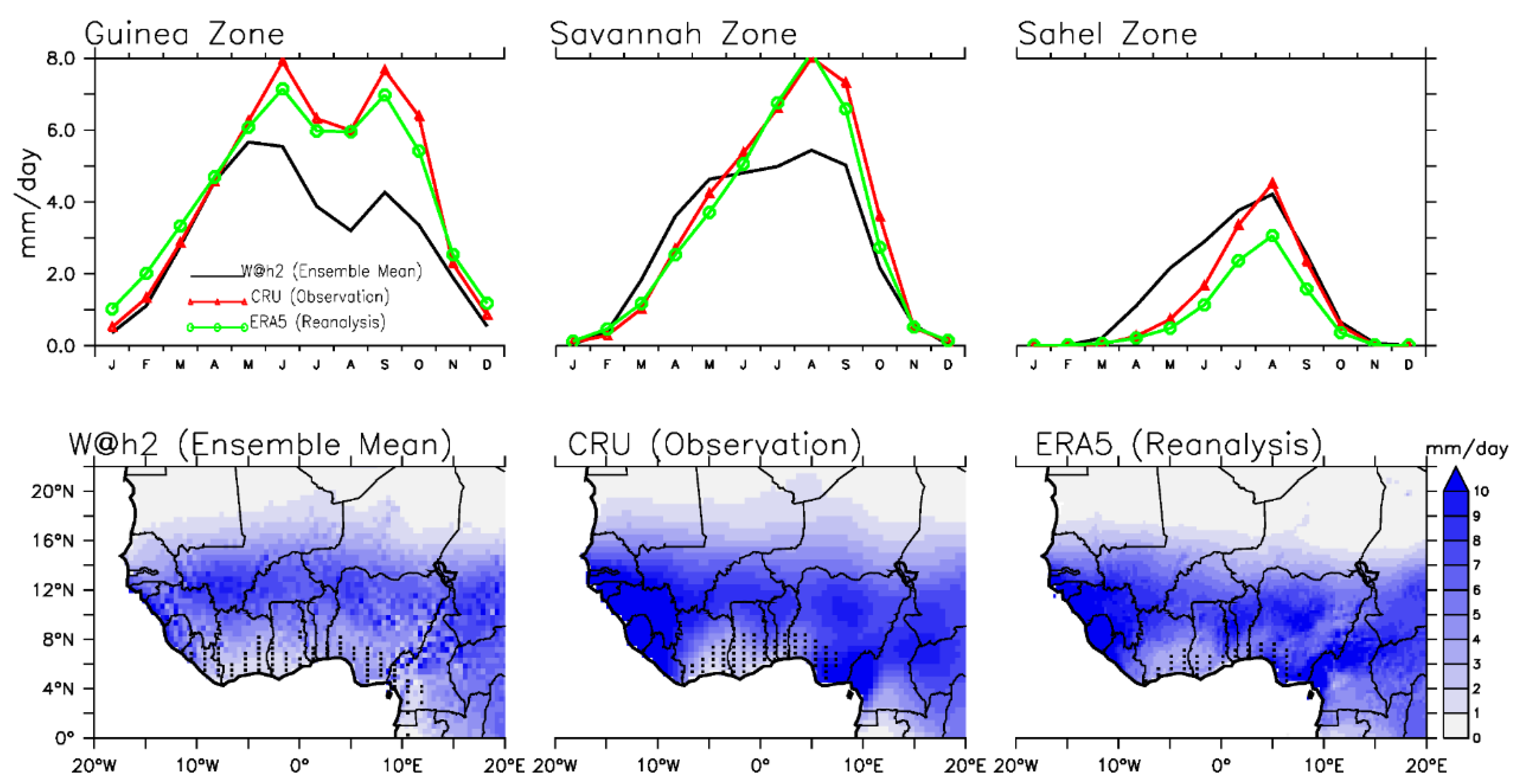
The w@h2 model is able to capture the monthly mean distributions of rainfall spatially and temporally (Figure 2 and Figure S1). As the rain band transverses hundreds of kilometers from south inland to north during the first half of the calendar year, w@h2 is able to capture the maximum rainfall along the coastal Guinea areas as well as the tropical aridity climates over the Sahel (Figure 2 and Figure S2a-c). The spatial correlations (r) between w@h2 simulations and CRU / ERA5 observations range from 0.68 to 0.85 (Figure S1a). While the model is able to simulate reliably the zenith characteristic of rainfall in August over both Savannah and Sahel, it is also able to capture the pause in rainfall intensities along the coastal Guinea areas in August – the little dry season (LDS: Figure 2 and Figure S1a-c). However, the LDS as simulated by w@h2 extends from Sierra Leone to southern Cameroon (Figure S1a) contrary to the Cote d’Ivoire to southeastern Nigeria extent as observed by CRU and ERA5 (Figure S1b, c).

Figure S2a shows that w@h2 rainfall over Guinea is consistently too low from June to October. Savannah rainfall is too high during March-May and too low during June-October (Figure S2b), while Sahel rainfall is too high from April to September (Figure S2c). The bias ranges of ±5mm day^-1 (Figure S2d, e) are small in comparison to rainfall totals over most of the region.

3.1.2. Temperature

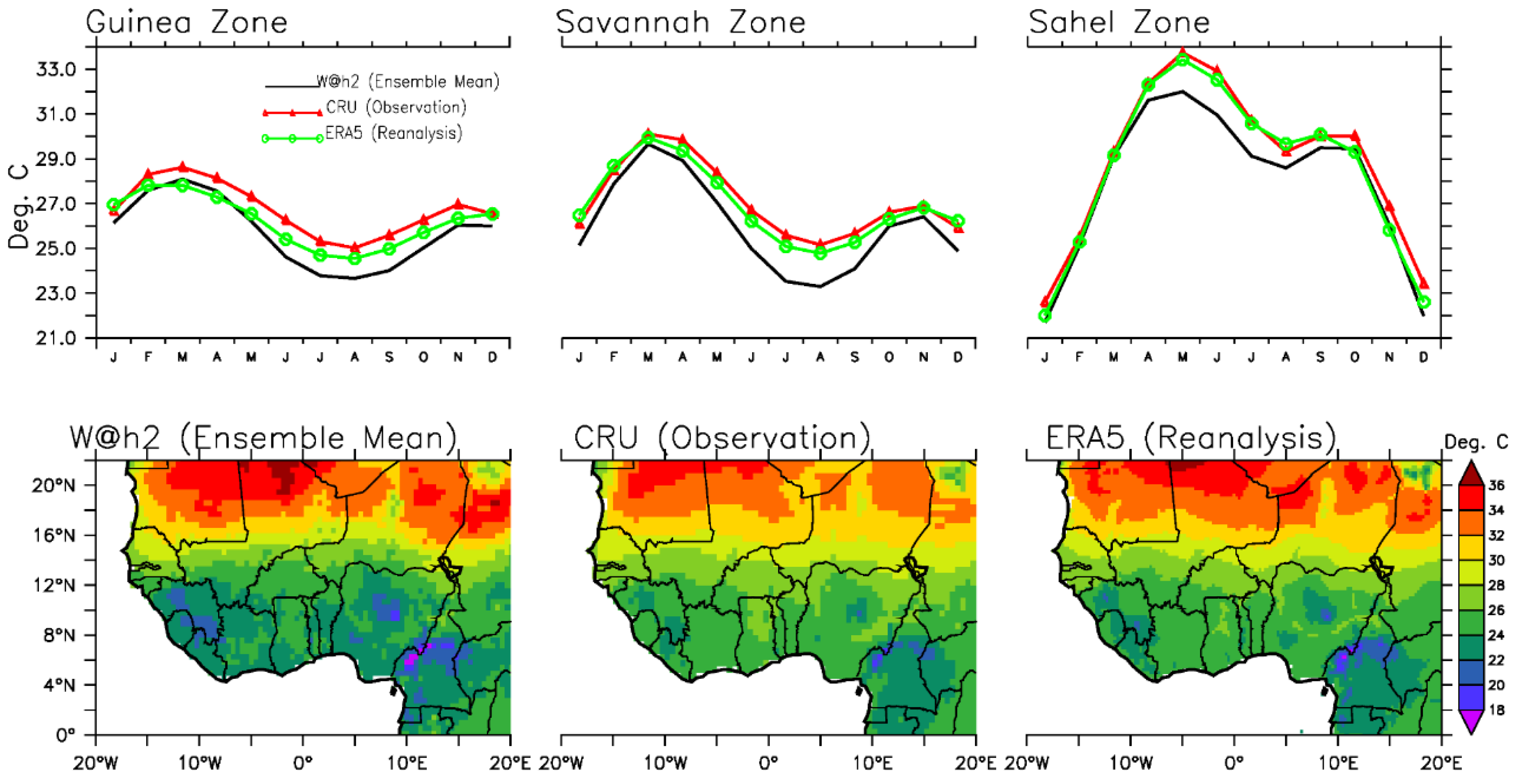
The spatial correlations (r) of the monthly temperature climatology between w@h2 simulations and CRU / ERA5 observations are generally greater than 0.9 (Figure S3a-c). w@h2 under-estimates the temperature in all climatic zones by 0.5-2.0°C (Figure S4a-e), though with patches of inconsistent over-estimations over the Sahel.

In addition, the w@h2 model captures the four main characteristics of the seasonal cycle of near surface maximum temperature over West Africa. First, the model captures the two peaks of maximum air temperature exhibited annually in all climatic zones, with the primary peak being in March-May with the secondary peak being in October-November (Figure 3, Figures S3a-c and S4a-c). Second, the model also agrees with observations that the Sahel region is always warmer than both the Savannah and coastal Guinea regions, except during the boreal winters. Third, the model agrees that there is a dip in the annual maximum temperatures over all climatic zones during the peak of the rainy season (i.e., in August: Figure 3 and Figure S3a-c). Lastly, the annual north-south oscillation of the thermal depression is also captured by the w@h2 model (Figure S3a-c); this being a large expanse of areas where the lowest atmospheric pressure coincides with surface temperature maximum (Figure 3, Parker et al. (2005), Lavaysse et al. (2009 and 2010)).

3.2. Association

Association, a statistical measure of the strength of a linear relationship between a paired simulation and observation / reanalysis data sets, is evaluated here by the use of spatio-temporal Pearson’s Product-Moment Correlation Coefficient (r) (Table 1). To a low extent, we also utilize the coefficient of determination (CoD) which is simply the square of r. CoD measures the level of skill attainable when the biases are eliminated.

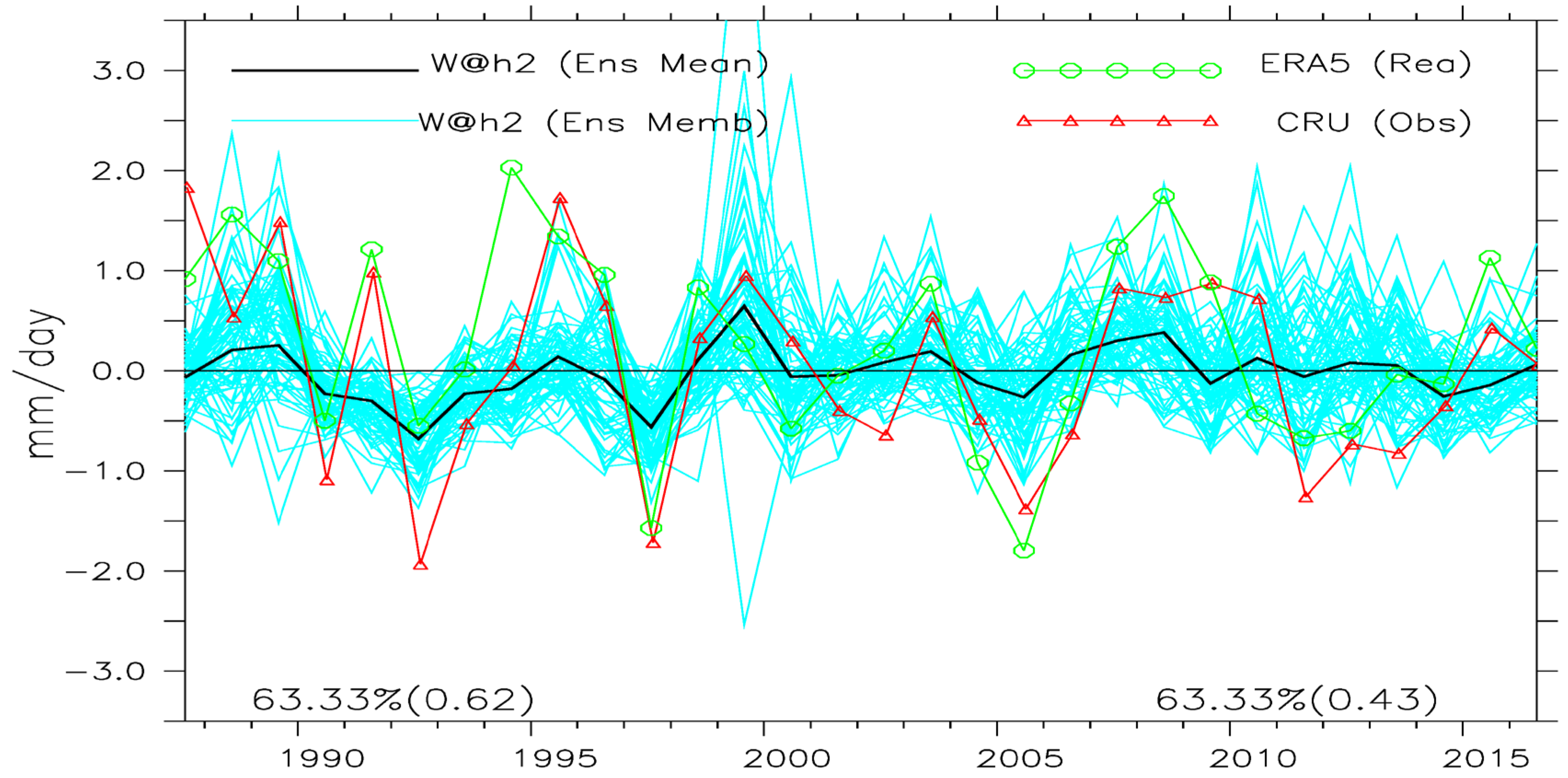
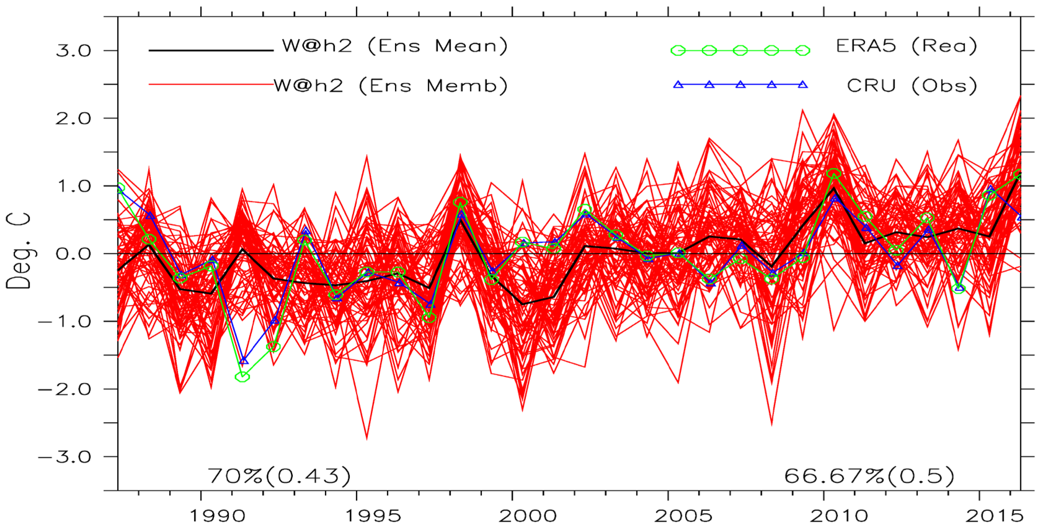
The inter-annual variability of Savannah rainfall and Sahel near surface maximum temperature, respectively, for the months of August and May are shown in Figure 4 (see Figure S5 for other months and zones). The observed (CRU/ERA5) values generally fall within the spread, notably during the unusually wet August 1999 over the Savannah and hot May 1998, 2010, and 2016 over the Sahel. There are some cases though when observed values are outside the spread of the ensemble members, such as the cool May 1991 over the Sahel.

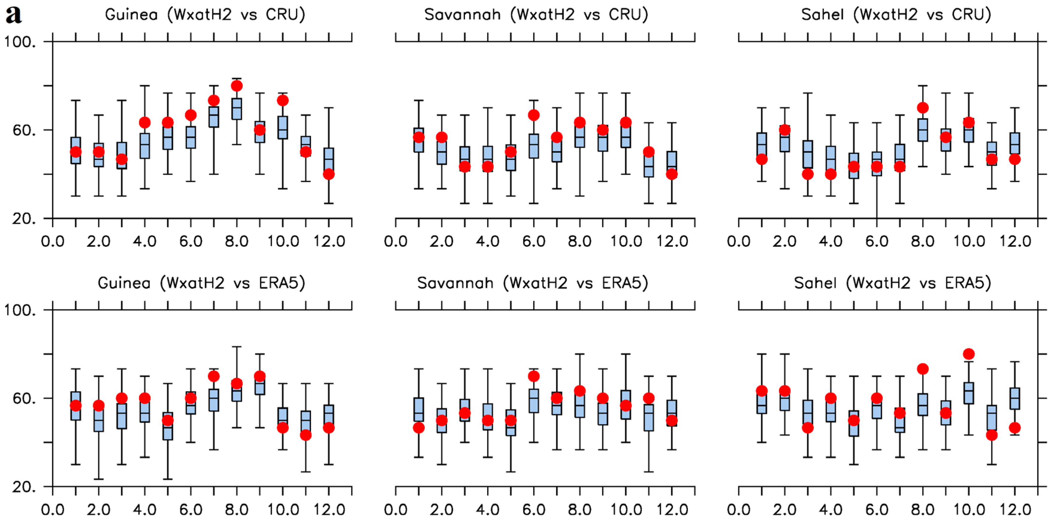
The linear relationship between w@h2 model’s temperature simulations and observations are strongly direct, while it is less strong for precipitation simulations. Correlations, r, values as large as 0.78 and 0.89 were evaluated for precipitation and temperature respectively, however cases of weak relationships, with r as low as ≈ -0.4 are also present, for individual simulations (Figure 4, and, Figure S5-7). Cases of weak relationships are more noticeable in the inter-annual variabilities of monthly precipitation simulations than in temperature (Figures S5-7). For both precipitation and temperature simulations, the strength of linear associations diminishes as we move to the drier north towards the Sahel (Figure 5 and Figure S5-8).

Irrespective of the magnitudes, the ability of the ensemble means of w@h2 model to capture the anomaly sign of the observed precipitation and temperature is generally greater than 40%, and at most 90% (Figure S5a-f). In other words, the model’s ensemble mean will adequately predict the sign of 2 out of 5 observations correctly; and will, at most, simulate about 9 out of 10 observations correctly (synchronization ≈ 90%).

The normalized standard deviations (NSD) of the majority of the ensemble members are greater than those of the ensemble means (Figures S6 and S7). This is because of the averaging that filters out the simulated variabilities of the ensemble means (Lawal, 2015; Lawal et al., 2019). These imply that the discrepancies between the ensemble means and observations, CRU/ERA5, are smaller than the discrepancies between individual ensemble members and observations.

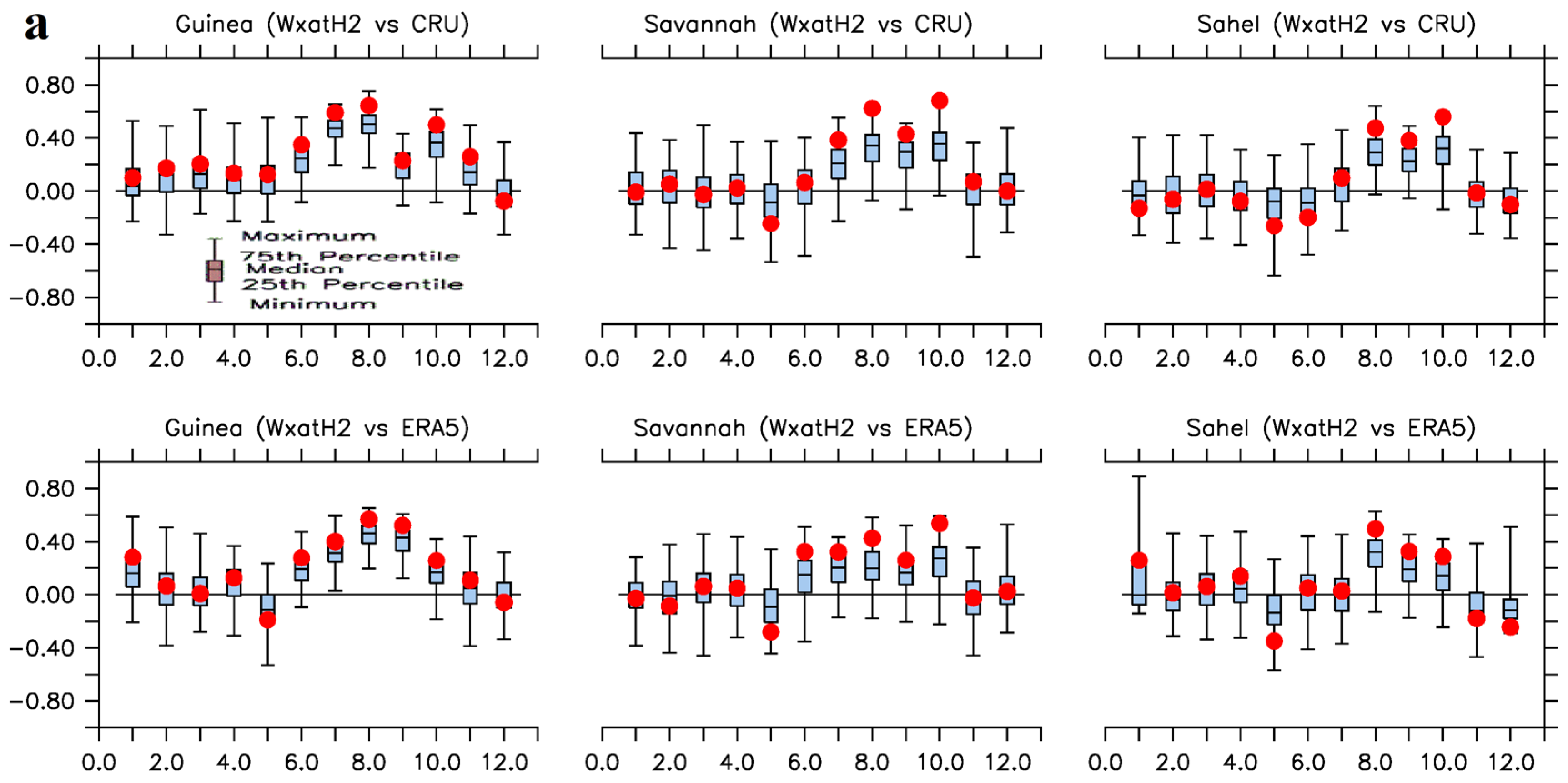
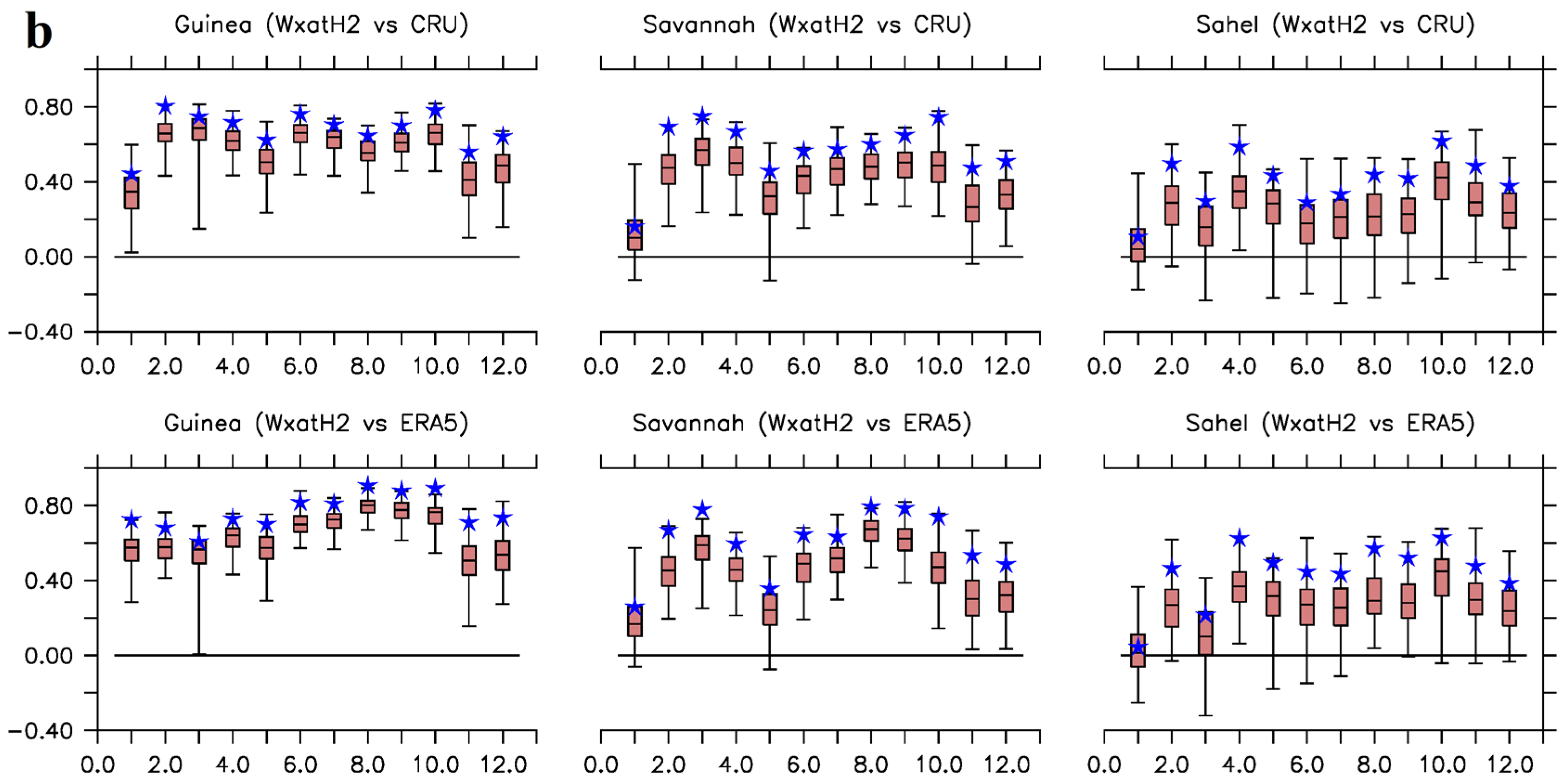
Furthermore, there are noticeable differences and similarities in the way w@h2 model’s precipitation and near surface maximum temperature simulations associate with observations (CRU/ERA5). Figure S8a-d shows that r between precipitation simulations and observations contain both direct and weak linear relationships, while cases of strong direct linear relationships dominate the r between the temperature simulations and observations. For instance, the correlations exhibited by the precipitation ensemble means are -0.4 < r < 0.78 while those of temperature are 0 < r < 0.8 (Figure 5a, b). Some of the precipitation ensemble means and members exhibited weak linear relationship with observations on monthly basis, except in July and August for CRU, and July, August and September for ERA5 over coastal Guinea (Figure 5a). This is however different for temperature simulations where all the ensemble means exhibited direct linear relationship, of various strength, with observations on monthly basis (Figure 5b). The best performance here is over Guinea where none of the temperature ensemble members had negative linear relationship with observations, i.e., 0 < r < 1.

Four similarities are typical to the associations of w@h2 model’s precipitation and temperature simulations with observations. Firstly, the CoD for both precipitation and temperature simulations are generally less than 0.5 (Figures not shown). Higher values, 0.5 < CoD < 0.8, are recorded during the peaks of the monsoon seasons. This corroborates the values of r, and implies that w@h2 model may also be skillful when biases are absent. Secondly, the spatio-temporal linear associations seem to strengthen with observations as rainfall seasons set in and stabilize. These are very obvious during the months of July, August and September (Figure S8a-d). Thirdly, the strength of linear associations, for both precipitation and temperature simulations, diminishes as we move north towards the Sahel. And lastly, all values of the associations of the ensemble means are enveloped by the spreads of the ensemble members’ associations (Figure 5). However, while the values of associations are generally greater than the 75th percentiles of the spreads in temperature simulations, they do not have any agreeably defined positions in precipitation simulations. The implications here are that the w@h2 model exhibits more significant associations during the peak of the West African monsoon seasons than the rest of the year. However, cautions are encouraged in terms of significant associations when applying the simulations over the Sahel.

Summarily for temperature, the ensemble mean always has a stronger correlation with observations than do most of the simulations; for precipitation, the rule seems to hold but maintain the sign of the correlation, i.e., a stronger anti-correlation when most simulations have negative r. The temperature’s positive correlation may be attributed to the strong warming trend over the experimental period (Cook and Vizy, 2015) while the weak correlations for precipitation may primarily reflect the inter-annual variability (Nicholson, 2001 and 2009).

3.3. Skill

The ranked probability skill score (RPSS) is here used to evaluate the ability of the w@h2 model to reproduce the observed monthly inter-annual variations in precipitations and near surface maximum temperature over West Africa (Table 1). RPSS measures the forecast accuracy with respect to a reference observation (e.g., observed climatology) as the scores reflect discrimination, reliability and resolution.

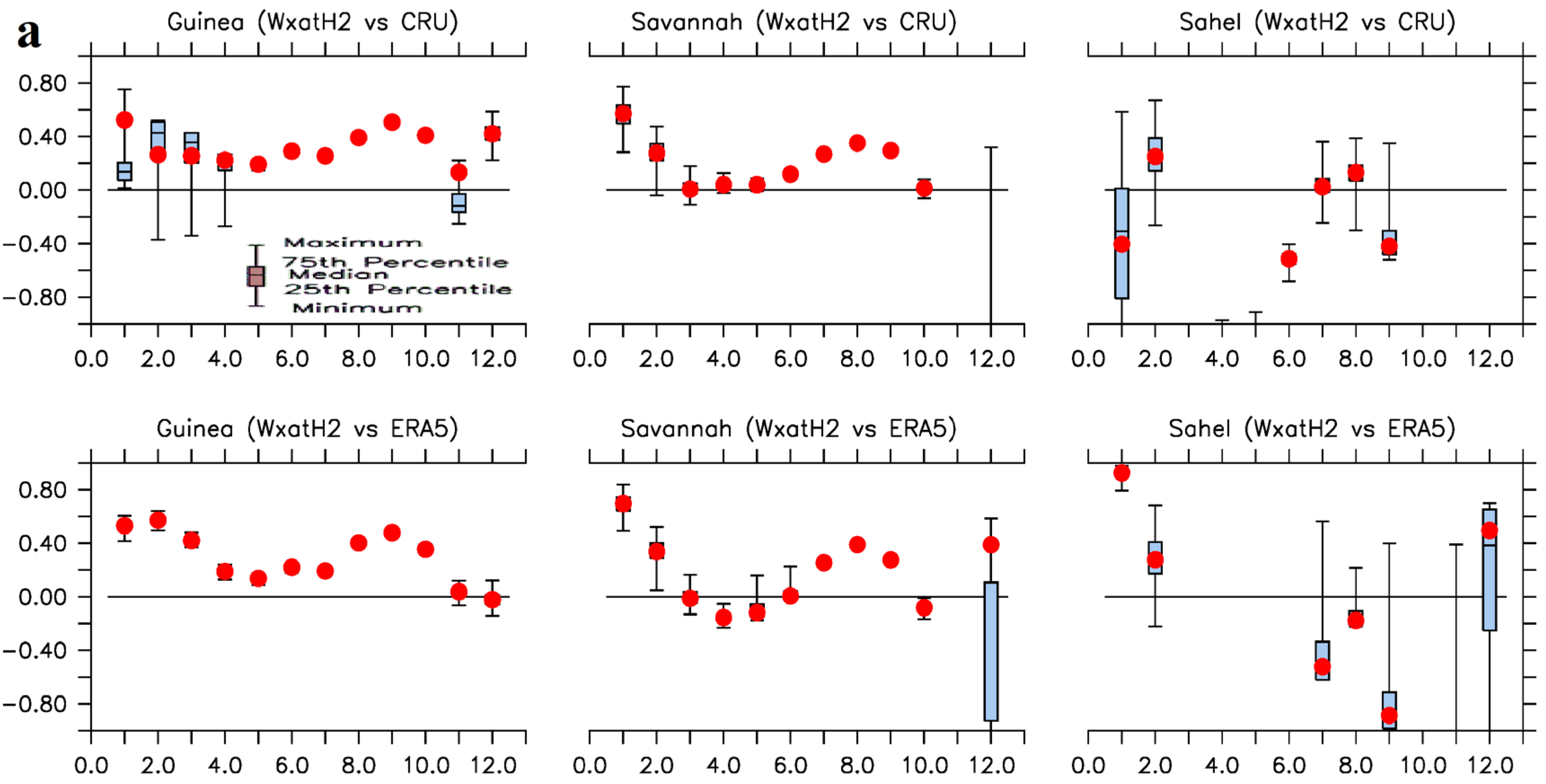
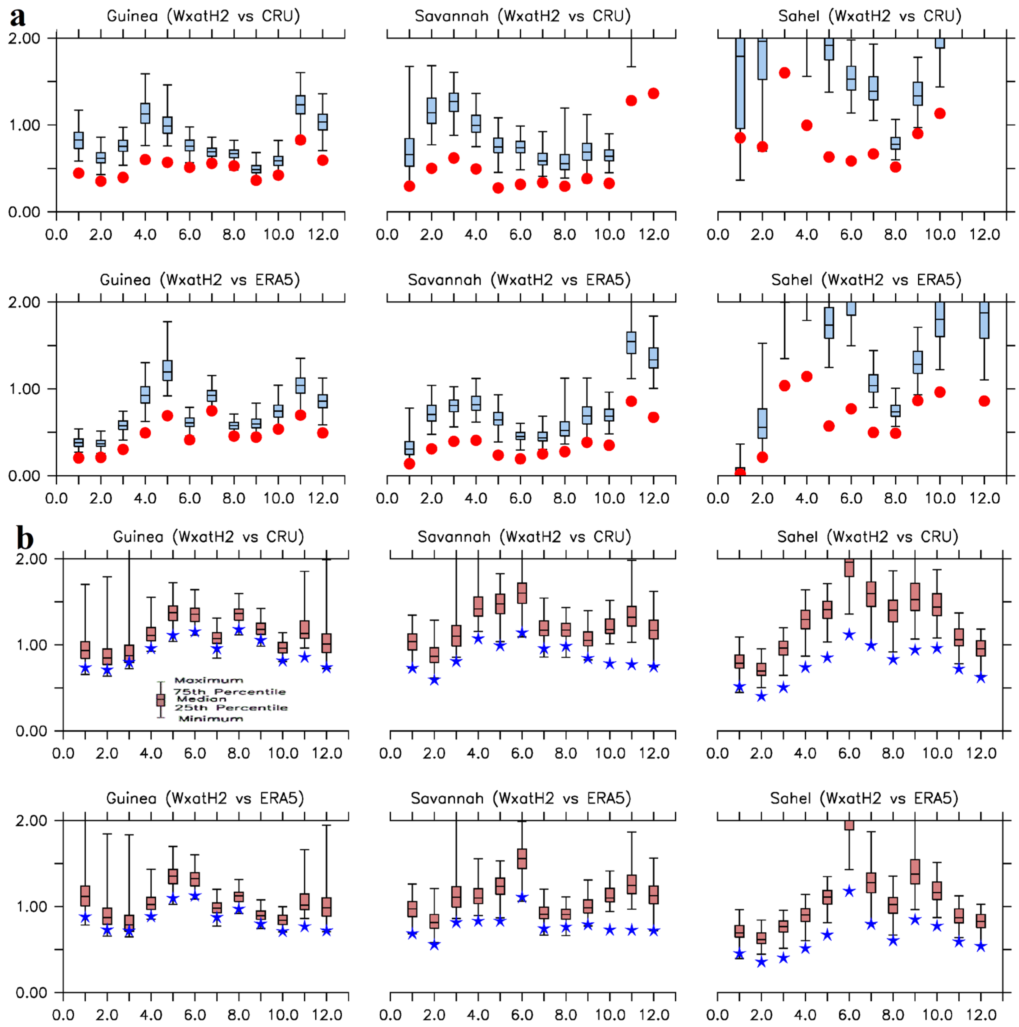
Positive skills, 0 < RPSS < 1, dominate Guinea and Savannah zones in all the months. However, reverse is the case over Sahel in precipitation simulations (Figure 6 and Figure S9). Nevertheless, all values of RPSS from ensemble means are within the spreads of the ensemble members’ RPSS; though, the spreads are of diverse thickness, the broadest being exhibited over Guinea zone. The ensemble means of the w@h2 model, with reference to the two observations (CRU/ERA5), returned positive values of RPSS for precipitation over Guinea throughout the year and positive values of RPSS for temperature over all the climatological zones, also throughout the year (except in January with reference to ERA5 over Sahel: Figure 6). Generally, while the skills of the w@h2 model with respect to precipitation simulations, over Sahel, may not be significantly impressive, the model may however have skills to detect heat waves that usually ravage West Africa during the boreal springs as well as skills to capture the LDS over Guinea zone.

3.4. Accuracy

As suggested by Walther and Moore (2005), we utilized mean absolute error (MAE), root mean square error (RMSE) and synchronization as measures to estimate accuracy in this paper. As tabulated in Table 1, MAE is a measure of the average magnitude of largest error that can be expected from a forecast without considering their directions. It is a linear score; meaning that all the individual differences are weighted equally in the average. Similar to MAE, RMSE also does not indicate the direction of the error, but it penalizes large errors. In contract, synchronization shows how much a simulated value agrees with an observed value in the signs of their anomalies without taking magnitudes into consideration.

The maximum average difference, as depicted by MAE, between the w@h2 model simulations and the observed (CRU/ERA5) precipitation over West Africa is about 5 mm day^-1 (Figure S10a, b). The average differences grow in values as rainfall season is setting in. High values of MAE, like 3 to 5 mm day^-1, are more vivid between the months of March to October and are more present in the southern coast of Guinea. In line with annual characteristics of rainfall, these high values migrate northward in a rainfall-like pattern and annual oscillation. Interestingly, they start to retreat southward in August/September. The relatively low values of MAE from November to February does not imply higher accuracy in rainfall estimation by the w@h2 model than the other months (Figure S10a, b); these are months of relatively very low precipitation (Figure 2 and Figure S1). The error magnitudes in precipitation do not represent up to 50% of over- or under-estimations in most parts of the sub-region. Therefore, w@h2 model cannot be labelled as a biased estimator of rainfall. Nevertheless, as recommended by Olaniyan et al. (2017), we may need to apply caution when utilizing ±30% of rainfall estimations as an indicator of biasness and accuracy.

The maximum average difference between the w@h2 model simulations and the observed (CRU/ERA5) near surface maximum temperature over West Africa is about 4^oC (Figure S10c, d). Generally, these differences are less than 2.8^oC. The higher values of MAE tend to occur in the early monsoon months of May, June, July and August, predominantly, over northern Savannah and southern parts of Sahel. The lower differences, MAE, that dominate the larger spatial expanse of West Africa, in all months, presumably make w@h2 model an accurate estimator of near surface maximum temperature.

There are sharp differences in RMSE and MAE produced from the precipitation simulations of w@h2 model. For example, the maximum RMSE in precipitation simulation is about 10 mm day^-1 (Figure S11a, b), while the maximum MAE is about 5 mm day^-1 (Figure S10a, b). This difference is, though, not large enough to indicate the presence of very large error in the simulation; it, nevertheless, signals that the precipitation simulations have large variance in the individual errors of its samples due to the existence of extreme precipitation values (the outliers). It is the outliers that introduces the random errors, i.e., the variability and or noise in the internal system of the precipitation simulations.

All errors are possibly of the same magnitudes in the near surface maximum temperature simulated by w@h2 model. This is because RMSE and MAE are almost equal in magnitudes (panels c and d of Figures S10 and S11). In similarity to MAE, RMSE are generally < 2.8^oC. This implies that it is the bias errors that are predominant here; meaning that the deviations in the temperature simulations, from observations, are not due to chance alone. They are rather systemic in nature. Exception here is in October – December over Sahel (Figure S11d), where there are sharp disagreements between CRU and ERA5 data sets (RMSE > 4^oC). Investigating the causes of this disagreements is outside the scope of this work.

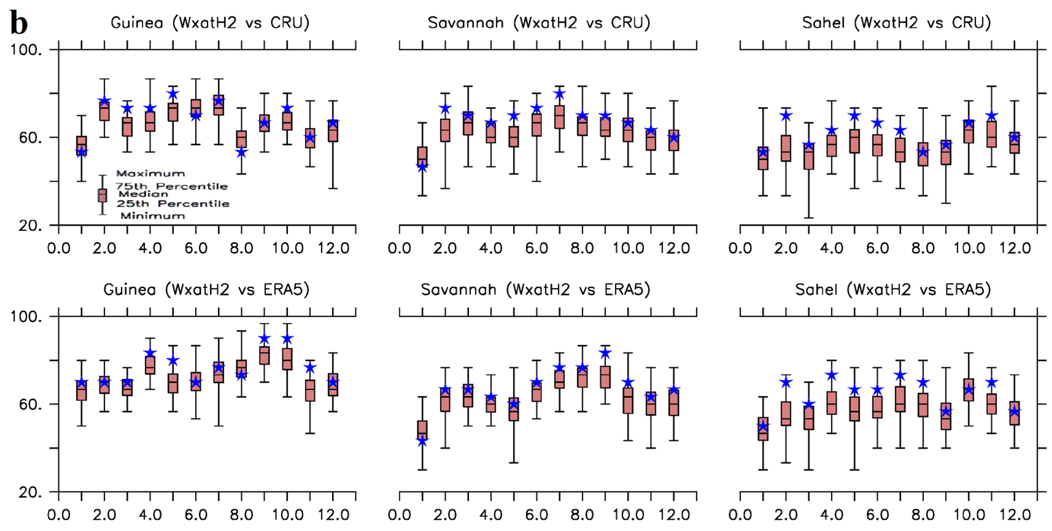
While corroborating the depictions on Figure S5a-f, Figure 7 and Figure S12 show that the abilities of w@h2 model to simulate the actual anomaly signs of the observed precipitation and near surface maximum temperature correctly is generally between 20 and 80% for precipitation ensemble members; and between 25 and 95% for temperature ensemble members. These imply that any ensemble member of w@h2 model, picked at random, will at worst / best simulate 1 out of 5 (synchronization ≈ 20%) / 4 out of 5 (synchronization ≈ 80%) actual signs of the anomalies correctly for precipitation; while, also at random, they will simulate at least 1 out of 4 (synchronization ≈ 25%) actual signs of the anomalies and at most more than 9 out of 10 (synchronization ≈ 95%) actual signs of the anomalies correctly for temperature. When combined, the model’s ensemble means of precipitation and temperature synchronize between 40% and 90% (Figure 7 and Figure S12). This shows that at worst they (i.e., the ensemble means) will simulate 2 out of 5 actual anomalies correctly, and will, at best, simulate 9 out of 10 actual signs of the anomalies correctly. Conclusively, while the w@h2 model may not be accurate in terms of getting the magnitudes of climate parameters right due to inherent presence of biases of different types, it may however be accurate in simulating the actual anomaly signs of the climate parameters rightly, to some significant extent. This is good because ability to reliably / accurately simulate the actual anomaly signs of observed climate parameters is one of the special attributes of a model that is needed for seasonal climate predictions and applications.

3.5. Precision

As shown on Table 1, precision is here evaluated with the use of coefficient of variation (CoV) and the normalized standard deviations (NSD). CoV, the ratio of standard deviations as measures of spreads to the mean of the sample populations, is used to determine the degrees of variability within the simulated and the observed climate parameters. Specifically, we employed the bias produced by CoV (i.e., CoV_model minus CoV_observation) to really know which of the two (simulations or observations) produces more spatio-temporal variabilities. NSD is used to measure the deviation factors between the simulations and the observations.

The degrees of spatio-temporal variability within the simulated and the observed climate parameters (precipitation and near surface maximum temperature) are depicted in Figure S13. The w@h2 model produces largely lesser spatio-temporal variabilities in precipitation in comparison to observations and almost normal deviations in spatio-temporal variabilities for temperature simulations. The largely sub-zero (≈ -50%) spatio-temporal variabilities are clearly evident in precipitation simulations as depicted by the biases of CoV (Figure S13a, b) over Savannah and Sahel zones; except during the months of July-August (peaks of raining season) when the CoV biases do not significantly deviate from zero (±10%), meaning that, during the monsoon seasons, the degrees of spatio-temporal variabilities around the mean is almost the same for precipitation simulations and observations.

Biases of CoV in temperature simulations range between ±1% (Figure S13c, d). Exceptions here are during the dry months of December-March, when largely negative CoV biases are visible over Savannah and Sahel zones. The implications of CoV biases, here, are that the degrees of spatio-temporal variabilities around the mean is almost the same for both temperature simulations and their observations during the wet seasons. Therefore, generally speaking, the w@h2 model simulations perform precisely well during monsoon seasons in terms of simulating precipitation and near surface maximum temperature. Summarily, on the average, the inter-annual variabilities of simulated w@h2 precipitation and near surface maximum temperature do not significantly exceed those of observations.

The discrepancies, as depicted by NSD, are majorly less than a factor of 1.0. As depicted on Figure 8, Figures S6 and S7, the discrepancies between the ensemble means and observations (i.e., CRU/ERA5), are smaller than the discrepancies between individual ensemble members and observations. For precipitation simulations, NSD is growing larger (> 1) as we move northwards towards Sahel zone (Figure 8a). Meanwhile, NSD tends to a factor of 1.0 as monsoon seasons are approached for temperature simulations (Figure 8b). This shows that there are little or negligible deviations between simulated and observed temperatures during the monsoon seasons. Generally, the majority of the ensemble means’ NSD values are outside the spreads of the ensemble members’ NSD; specifically, below the first percentiles (the minimum on the error bars). These behaviors on the path of the ensemble means confirm the “precise nature” of the ensemble means over the members as already documented (e.g., Ehrendorfer, 1997; Hamil and Colucci, 1997; Palmer, 2000; Stensrud et al., 2000; Stensrud and Yussouf, 2003; Jankov et al., 2005).

4. Summary and Discussion

This study is motivated by the generation of a remarkably huge ensemble of simulations, counting more than 10,000 ensemble members. The achievement allows denser sampling of the climate distributions, allowing more precise calculation of climate model properties. We seek to provide a performance evaluation of the w@h2 simulations over West Africa using the framework of RASAP (reliability, association, skill, accuracy, and precision) measures.

Results show that, to some significant extent, w@h2 model provides little, if any, predictive information for precipitation during the dry season, but may provide useful information during the monsoon seasons. This means that a prospective user gets to decide whether it is “useful” for his/her particular application. This evaluation provides a prospective user with information that he/she can use to decide whether the model might be “useful or not”. For instance, a prospective user may ignore rainfall simulations during the dry seasons (when there are not much to predict), but consider it for the wet seasons. Contrary to the results for precipitation, w@h2 model provides sufficient predictive information for the near surface maximum temperature over West Africa throughout the year. For example, the model is able to reproduce all the annual characteristics of maximum air temperature such as 1. the two peaks of maximum air temperature over all the climatic zones; 2. the Sahel being the warmest of all the zones, except during the boreal winters; 3. the dip in the annual maximum temperatures over all climatic zones during the peak of the rainy season; and 4. the annual north-south oscillation of the thermal depression.

Analyses carried out in this paper have provided some statistical insights to the nature of the w@h2 simulations over West African region. The w@h2 modelling system was designed for the investigation of the behavior of extreme weather under anthropogenic climate change, i.e., event attribution. For event attribution, as earlier stated, measures of the performance of a model in terms of climate variability may be more relevant than measures of the mean climatology (Bellprat and Doblas-Reyes, 2016; Lott and Stott, 2016; Bellprat et al., 2019). Therefore, w@h2 model is unique in producing large sample sizes that are able to show that sampling quality of the tails of the distribution is no longer the primary constraint / source of uncertainty.

Bellprat and Doblas-Reyes (2016) and Bellprat et al. (2019) point out that if the unforced variability of a model, in comparison to observation, is too small / large then the model will be too keen / not keen enough to attribute an event’s occurrence to emissions. Here, the unsubstantial bias and low variability in its precipitation and temperature simulations present the model as too keen to attribute an event to emissions. In addition, high skills, especially during the monsoon seasons, may probably mean that there is a lot of predictability in the system. Therefore, for an SST-forced system like w@h2, this means that event attribution conclusions are conditional on the occurrence of the observed SST state (Risser et al., 2017).

Furthermore, lack of obvious quality of the model in terms of rain during the dry seasons may not mean that it has a bias for event attribution analysis. It may only mean that there are no evidences that strongly supports the notion that the model is accurately simulating the appropriate processes for extremes. But, on the contrary, predictive skills for the onset season suggest that the model is getting processes right.

Investigating the reasons for the model’s deficiencies is beyond the scope of this work. The investigation shall be attended to in the second part of this work, where we intend to consider the model’s reproducibility of atmospheric dynamics that influence and modulate West African weather and climate. Then, we will fully be able to say if the model is doing a reasonable job of capturing processes over West Africa.

Author Contributions

All authors listed have approved this work for publication, having made a substantial direct and intellectual contribution to the work in the order of activities listed against their names as follow: KAL conceptualization, investigation, methodology, validation, resources, writing (original draft, review and editing), visualization, software, formal analysis, data processing and supervision. OMA investigation, writing (editing), visualization and data processing. EO methodology, writing (review), software, formal analysis, visualization and data processing. AB and SNS resources, validation, writing (review and editing) and project administration. MFW and DAS conceptualization, investigation, methodology, validation, resources, writing (review and editing), supervision and project administration.

Data Availability Statement

The raw data supporting the conclusions of this article will be made available by the authors on request, without undue reservation.

Acknowledgments

KAL was supported by the Intra-ACP Climate Services and Related Applications (ClimSA: https://www.climsa.org/) Program in Africa, an initiative funded by the European Union’s 11th European Development Fund and implemented by the African Centre of Meteorological Applications for Development through a grant with the African Union Commission as the contracting authority; and, the BNP Attribution Project of the African Climate and Development Initiative (ACDI: www.acdi.uct.ac.za) of the University of Cape Town, South Africa. MFW was supported by the Director, Office of Science, Office of Biological and Environmental Research of the U.S. Department of Energy as part of the Regional and Global Model Analysis program under Contract No. DE340AC02-05CH11231. DAS was supported by the Whakahura project funded by the New Zealand Ministry of Business, Innovation, and Employment. The authors gratefully acknowledge the computational, technical and infrastructural supports provided by the Climate Sciences Analysis Group (CSAG: www.csag.uct.ac.za), University of Cape Town, South Africa. We are also thanking all reviewers whose comments helped to improve the quality of this manuscript.

Conflicts of Interest

The authors declare that the research was conducted in the absence of any commercial or financial relationships that could be construed as a potential conflict of interest.

References

Afiesimama, E.A. Annual cycle of the mid-tropospheric easterly jet over West Africa. Theor. Appl. Clim. 2007, 90, 103–111. [Google Scholar] [CrossRef]
Anderson, DP. 2004. Boinc: A system for public-resource computing and storage, in: Fifth IEEE/ACM International Workshop on Grid Computing, IEEE, 4–10.
Bellprat, O.; Doblas-Reyes, F. Attribution of extreme weather and climate events overestimated by unreliable climate simulations. Geophys. Res. Lett. 2016, 43, 2158–2164. [Google Scholar] [CrossRef]
Bellprat, O.; Guemas, V.; Doblas-Reyes, F.; Donat, M.G. Towards reliable extreme weather and climate event attribution. Nat. Commun. 2019, 10, 1–7. [Google Scholar] [CrossRef] [PubMed]
Brose, U.; Martinez, N.D.; Williams, R.J. Estimating species richness: sensitivity to sample coverage and insensitivity to spatial patterns. Ecology 2003, 84, 2364–2377. [Google Scholar] [CrossRef]
Camberlin, P.; Janicot, S.; Poccard, I. Seasonality and atmospheric dynamics of the teleconnection between African rainfall and tropical sea-surface temperature: Atlantic vs. ENSO. Int. J. Clim. 2001, 21, 973–1005. [Google Scholar] [CrossRef]
Cook, K.H.; Vizy, E.K. Detection and Analysis of an Amplified Warming of the Sahara Desert. J. Clim. 2015, 28, 6560–6580. [Google Scholar] [CrossRef]
Debanne, S.M. The planning of clinical studies: Bias and precision. Gastrointest. Endosc. 2000, 52, 821–822. [Google Scholar] [CrossRef]
Diallo, I.; Bain, C.L.; Gaye, A.T.; Moufouma-Okia, W.; Niang, C.; Dieng, M.D.B.; Graham, R. Simulation of the West African monsoon onset using the HadGEM3-RA regional climate model. Clim. Dyn. 2014, 43, 575–594. [Google Scholar] [CrossRef]
Diallo, I.; Sylla, M.B.; Camara, M.; Gaye, A.T. Interannual variability of rainfall over the Sahel based on multiple regional climate models simulations. Theor. Appl. Clim. 2012, 113, 351–362. [Google Scholar] [CrossRef]
Diedhiou, A.; Janicot, S.; Viltard, A.; de Felice, P. Evidence of two regimes of easterly waves over West Africa and the tropical Atlantic. Geophys. Res. Lett. 1998, 25, 2805–2808. [Google Scholar] [CrossRef]
Ebert, E.; Wilson, L.; Weigel, A.; Mittermaier, M.; Nurmi, P.; Gill, P.; Göber, M.; Joslyn, S.; Brown, B.; Fowler, T.; et al. Progress and challenges in forecast verification. Meteorol. Appl. 2013, 20, 130–139. [Google Scholar] [CrossRef]
Ehrendorfer, M. Predicting the uncertainty of numerical weather forecasts: A review. Meteor. Z. 1997, 6, 147–183. [Google Scholar] [CrossRef]
Grist, J.P.; Nicholson, S.E.; Barcilon, A.I. Easterly Waves over Africa. Part II: Observed and Modeled Contrasts between Wet and Dry Years. Mon. Weather. Rev. 2002, 130, 212–225. [Google Scholar] [CrossRef]
Guillod, B.P.; Jones, R.G.; Bowery, A.; Haustein, K.; Massey, N.R.; Mitchell, D.M.; Otto, F.E.L.; Sparrow, S.N.; Uhe, P.; Wallom, D.C.H.; et al. weather@home 2: validation of an improved global–regional climate modelling system. Geosci. Model Dev. 2017, 10, 1849–1872. [Google Scholar] [CrossRef]
Hamill, T.M.; Colucci, S.J. Verification of Eta–RSM Short-Range Ensemble Forecasts. Mon. Weather. Rev. 1997, 125, 1312–1327. [Google Scholar] [CrossRef]
Harris, I.; Jones, P.D.; Osborn, T.J.; Lister, D.H. Updated high-resolution grids of monthly climatic observations—The CRU TS3.10 Dataset. Int. J. Climatol. 2014, 34, 623–642. [Google Scholar] [CrossRef]
Hersbach H, de Rosnay P, Bell B, Schepers D, Simmons A, Soci C, Abdalla S, Balmaseda MA, Balsamo G, Bechtold P, Berrisford P, Bidlot J, de Boisséson E, Bonavita M, Browne P, Buizza R, Dahlgren P, Dee D, Dragani R, Diamantakis M, Flemming J, Forbes R, Geer A, Haiden T, Hólm E, Haimberger L, Hogan R, Horányi A, Janisková M, Laloyaux P, Lopez P, Muñoz-Sabater J, Peubey C, Radu R, Richardson D, Thépaut J-N, Vitart F, Yang X, Zsótér E, Zuo H. 2018. Operational global reanalysis: progress, future directions and synergies with NWP. ERA Report Series, No. 27, ECMWF.
Hidore JJ, Oliver JE, Snow M, Snow Richard. 2009. Climatology: An Atmospheric Science. 3rd Edition. Pearson, California, USA. ISBN-10: 0321602056. ISBN-13: 978-0321602053.
Jankov I, Gallus Jr. WA, Segal M, Shaw B, Koch SE. 2005. The impact of different WRF model physical parameterizations and their interactions on warm season MCS rainfall. Wea. Forecasting, 20, 1048–1060.
Jolliffe, I.T.; Stephenson, D.B. Forecast Verification: A Practitioner’s Guide in Atmospheric Science. 1st Edition. John Wiley & Sons, Ltd. Print ISBN:9780470660713. Online ISBN:9781119960003. 2012. [Google Scholar] [CrossRef]
Jones RG, Noguer M, Hassell DC, Hudson D, Willson SS, Genkins GJ, Mitchell JFB. 2004. Generating high resolution climate change scenarios using PRECIS. Technical report, Met Office Hadley Centre, Exeter, UK, 40 pp.
Kim, G.; Ahn, J.-B.; Kryjov, V.N.; Sohn, S.-J.; Yun, W.-T.; Graham, R.; Kolli, R.K.; Kumar, A.; Ceron, J.-P. Global and regional skill of the seasonal predictions by WMO Lead Centre for Long-Range Forecast Multi-Model Ensemble. Int. J. Climatol. 2016, 36, 1657–1675. [Google Scholar] [CrossRef]
Klein, C.; Heinzeller, D.; Bliefernicht, J.; Kunstmann, H. Variability of West African monsoon patterns generated by a WRF multi-physics ensemble. Clim. Dyn. 2015, 45, 2733–2755. [Google Scholar] [CrossRef]
Latif, M.; Grötzner, A. The equatorial Atlantic oscillation and its response to ENSO. Clim. Dyn. 2000, 16, 213–218. [Google Scholar] [CrossRef]
Lavaysse, C.; Diedhiou, A.; Laurent, H.; Lebel, T. African Easterly Waves and convective activity in wet and dry sequences of the West African Monsoon. Clim. Dyn. 2006, 27, 319–332. [Google Scholar] [CrossRef]
Lavaysse, C.; Flamant, C.; Janicot, S.; Parker, D.J.; Lafore, J.-P.; Sultan, B.; Pelon, J. Seasonal evolution of the West African heat low: a climatological perspective. Clim. Dyn. 2009, 33, 313–330. [Google Scholar] [CrossRef]
Lavaysse, C.; Flamant, C.; Janicot, S.; Knippertz, P. Links between African easterly waves, midlatitude circulation and intraseasonal pulsations of the West African heat low. Q. J. R. Meteorol. Soc. 2010, 136, 141–158. [Google Scholar] [CrossRef]
Lawal, KA. 2015. Understanding the Variability and Predictability of Seasonal Climates over West and Southern Africa using Climate Models. PhD thesis, Faculty of Sciences, University of Cape Town, South Africa. Available online at: https://open.uct.ac.za/handle/11427/16556?show=full.
Lawal, K.A.; Abiodun, B.J.; Stone, D.A.; Olaniyan, E.; Wehner, M.F. Capability of CAM5.1 in simulating maximum air temperature anomaly patterns over West Africa during boreal spring. Model. Earth Syst. & Environ., 2019, 5, 1815-1838. https://doi.org/10.1007/s40808-019-00639-2. Lott FC, Stott PA. Evaluating Simulated Fraction of Attributable Risk Using Climate Observations. J. Climate 2016, 29, 4565–4575. [Google Scholar] [CrossRef]
Mariotti, L.; Coppola, E.; Sylla, M.B.; Giorgi, F.; Piani, C. Regional climate model simulation of projected 21st century climate change over an all-Africa domain: Comparison analysis of nested and driving model results. J. Geophys. Res. Atmos. 2011, 116. [Google Scholar] [CrossRef]
Mason, S.J. On Using “Climatology” as a Reference Strategy in the Brier and Ranked Probability Skill Scores. Mon. Weather. Rev. 2004, 132, 1891–1895. [Google Scholar] [CrossRef]
Mason, S.J. Understanding forecast verification statistics. Meteorol. Appl. 2008, 15, 31–40. [Google Scholar] [CrossRef]
Massey, N.; Jones, R.; Otto, F.E.L.; Aina, T.; Wilson, S.; Murphy, J.M.; Hassell, D.; Yamazaki, Y.H.; Allen, M.R. weather@home—development and validation of a very large ensemble modelling system for probabilistic event attribution. Q. J. R. Meteorol. Soc. 2014, 141, 1528–1545. [Google Scholar] [CrossRef]
Melo, A.S.; Pereira, R.A.S.; Santos, A.J.; Shepherd, G.J.; Machado, G.; Medeiros, H.F.; Sawaya, R.J. Comparing species richness among assemblages using sample units: why not use extrapolation methods to standardize different sample sizes? Oikos 2003, 101, 398–410. [Google Scholar] [CrossRef]
Misra, J. Phase synchronization. Inf Process Lett. 1991, 38, 101–105. [Google Scholar] [CrossRef]
Murphy, AH. Skill score on the mean square error and their relationship to the correlation coefficient. Monthly Weather Review 1988, 116, 2417–2424. [Google Scholar] [CrossRef]
Murphy, A.H. The Coefficients of Correlation and Determination as Measures of performance in Forecast Verification. Weather. Forecast. 1995, 10, 681–688. [Google Scholar] [CrossRef]
New M, Hulme M, Jones PD. 2000. Representing twentieth century space-time climate variability. Part 2: development of 1901-96 monthly grids of terrestrial surface climate. Journal of Climate, 13, 2217–2238. [CrossRef]
Newman M, Sardeshmukh PD, Winkler CR, Whitaker JS. 2003. A study of sub-seasonal predictability. Mon. Wea. Rev., 131, 1715–1732. [CrossRef]
Niang I, Ruppel O, Abdrabo M, Essel A, Lennard C, Padgham J, Urquhart P. 2014. Africa, climate change 2014: impacts, adaptation and vulnerability – Contributions of the Working Group II to the Fifth Assessment Report of the Intergovernmental Panel on Climate Change. 1199–1265.
Nicholson, S.E. An Overview of African Rainfall Fluctuations of the Last Decade. J. Clim. 1993, 6, 1463–1466. [Google Scholar] [CrossRef]
Nicholson SE, Palao IM. 1993. A Re-evaluation of rainfall variability in the Sahel. Part I. Characteristics of rainfall fluctuations. International Journal of Climatology 13: 371–389.
Nicholson, SE. 1995. Sahel, West Africa. Encyclopedia of Environmental Biology 3: 261–275.
Nicholson, S. Climatic and environmental change in Africa during the last two centuries. Clim. Res. 2001, 17, 123–144. [Google Scholar] [CrossRef]
Nicholson, S.E.; Grist, J.P. The Seasonal Evolution of the Atmospheric Circulation over West Africa and Equatorial Africa. J. Clim. 2003, 16, 1013–1030. [Google Scholar] [CrossRef]
Nicholson, S.E. On the factors modulating the intensity of the tropical rainbelt over West Africa. Int. J. Clim. 2008, 29, 673–689. [Google Scholar] [CrossRef]
Nikulin, G.; Jones, C.; Giorgi, F.; Asrar, G.; Büchner, M.; Cerezo-Mota, R.; Christensen, O.B.; Déqué, M.; Fernandez, J.; Hänsler, A.; et al. Precipitation climatology in an ensemble of CORDEX-Africa regional climate simulations. J. Clim. 2012, 25, 6057–6078. [Google Scholar] [CrossRef]
Nkiaka, E.; Taylor, A.L.; Dougill, A.J.; Antwi-Agyei, P.; Fournier, N.; Bosire, E.N.; Konte, O.; Lawal, K.A.; Mutai, B.; Mwangi, E.; et al. Identifying user needs for weather and climate services to enhance resilience to climate shocks in sub-Saharan Africa. Environ. Res. Lett. 2019, 14, 123003. [Google Scholar] [CrossRef]
Odekunle, T.O.; Eludoyin, A.O. Sea surface temperature patterns in the Gulf of Guinea: their implications for the spatio-temporal variability of precipitation in West Africa. Int. J. Clim. 2008, 28, 1507–1517. [Google Scholar] [CrossRef]
Olaniyan, E.; Adefisan, E.A.; Oni, F.; Afiesimama, E.; Balogun, A.A.; Lawal, K.A. Evaluation of the ECMWF Sub-seasonal to Seasonal Precipitation Forecasts during the Peak of West Africa Monsoon in Nigeria. Front. Environ. Sci. 2017, 6, 1–15. [Google Scholar] [CrossRef]
Omotosho, J.B. Pre-rainy season moisture build-up and storm precipitation delivery in the West African Sahel. Int. J. Clim. 2007, 28, 937–946. [Google Scholar] [CrossRef]
Omotosho, J.B.; Abiodun, B.J. A numerical study of moisture build-up and rainfall over West Africa. Meteorol. Appl. 2007, 14, 209–225. [Google Scholar] [CrossRef]
Palmer, T.N. Predicting uncertainty in forecasts of weather and climate. Rep. Prog. Phys. 2000, 63, 71–116. [Google Scholar] [CrossRef]
Parker, D.J.; Thorncroft, C.D.; Burton, R.R.; Diongue-Niang, A. Analysis of the African easterly jet, using aircraft observations from the JET2000 experiment. Q. J. R. Meteorol. Soc. 2005, 131, 1461–1482. [Google Scholar] [CrossRef]
Pledger, S. Unified maximum likelihood estimates for cloud capture-recapture models using mixtures. Biometrics 2000, 56, 434–442. [Google Scholar] [CrossRef]
Pledger, S.; Schwarz, C.J. Modelling heterogeneity of survival in band-recovery data using mixtures. J. Appl. Stat. 2002, 29, 315–327. [Google Scholar] [CrossRef]
Redelsperger, J.-L.; Thorncroft, C.D.; Diedhiou, A.; Lebel, T.; Parker, D.J.; Polcher, J. African Monsoon Multidisciplinary Analysis: An International Research Project and Field Campaign. Bull. Am. Meteorol. Soc. 2006, 87, 1739–1746. [Google Scholar] [CrossRef]
Risser, M.D.; Stone, D.A.; Paciorek, C.J.; Wehner, M.F.; Angélil, O. Quantifying the effect of interannual ocean variability on the attribution of extreme climate events to human influence. Clim. Dyn. 2017, 49, 3051–3073. [Google Scholar] [CrossRef]
Rosenberg, D.K.; Overton, W.S.; Anthony, R.G. Estimation of Animal Abundance When Capture Probabilities Are Low and Heterogeneous. J. Wildl. Manag. 1995, 59, 252. [Google Scholar] [CrossRef]
Stensrud DJ, Bao J-W, Warner TT. Using initial condition and model physics perturbations in short-range ensemble simulations of mesoscale convective systems. Mon. Wea. Rev. 2000, 128, 2077–2107. [CrossRef]
Stensrud DJ, Yussouf N. 2003. Short-range ensemble predictions of 2-m temperature and dew-.
point temperature over New England. Mon. Wea. Rev., 131, 2510–2524.
Storch HV, Zwiers FW. 2003. Statistical analysis in climate research. Cambridge University Press, London.
Sylla, M.B.; Giorgi, F.; Pal, J.S.; Gibba, P.; Kebe, I.; Nikiema, M. Projected Changes in the Annual Cycle of High-Intensity Precipitation Events over West Africa for the Late Twenty-First Century*. J. Clim. 2015, 28, 6475–6488. [Google Scholar] [CrossRef]
Tall, A.; Mason, S.J.; van Aalst, M.; Suarez, P.; Ait-Chellouche, Y.; Diallo, A.A.; Braman, L. Using Seasonal Climate Forecasts to Guide Disaster Management: The Red Cross Experience during the 2008 West Africa Floods. Int. J. Geophys. 2012, 2012, 1–12. [Google Scholar] [CrossRef]
Walther, B.A.; Moore, J.L. The concepts of bias, precision and accuracy, and their use in testing the performance of species richness estimators, with a literature review of estimator performance. Ecography 2005, 28, 815–829. [Google Scholar] [CrossRef]
Weigel, A.P.; Liniger, M.A.; Appenzeller, C. The Discrete Brier and Ranked Probability Skill Scores. Mon. Weather. Rev. 2007, 135, 118–124. [Google Scholar] [CrossRef]
West, M.J. Stereological methods for estimating the total number of neurons and synapses: issues of precision and bias. Trends Neurosci. 1999, 22, 51–61. [Google Scholar] [CrossRef] [PubMed]
Wilks, DS. 1995. Statistical Methods in Atmospheric Sciences: An Introduction, 2nd Edition. Academic Press: San Diego, CA.
Wilson, L.J.; Giles, A. A new index for the verification of accuracy and timeliness of weather warnings. Meteorol. Appl. 2013, 20, 206–216. [Google Scholar] [CrossRef]
Xue, Y.; De Sales, F.; Lau, W.K.-M.; Boone, A.; Feng, J.; Dirmeyer, P.; Guo, Z.; Kim, K.-M.; Kitoh, A.; Kumar, V.; et al. Intercomparison of West African Monsoon and its variability in the West African Monsoon Modelling Evaluation Project (WAMME) first model inter-comparison experiment. Clim. Dyn. 2010, 35, 3–27. [Google Scholar] [CrossRef]
Zaroug, M.A.H.; Sylla, M.B.; Giorgi, F.; Eltahir, E.A.B.; Aggarwal, P.K. A sensitivity study on the role of the swamps of southern Sudan in the summer climate of North Africa using a regional climate model. Theor. Appl. Clim. 2012, 113, 63–81. [Google Scholar] [CrossRef]
Zelmer, D.A.; Esch, G.W. Robust estimation of parasite component community richness. J. Parasitol. 1999, 85, 592–594. [Google Scholar] [CrossRef]

Figure 1. The domain of West Africa showing the topography of the surface (shaded; meters) and highlights of climatological zones – Guinea (green box), Savannah (blue box), and Sahel (red box).

Figure 2. (Top panels) Aerial averages of monthly mean distributions of rainfall (mm day^-1) for each climatological zone: left) Guinea, middle) Savannah, and right) Sahel. (Bottom panels) Mean spatial distributions of rainfall (shaded; mm day^-1) over West Africa for the month of August: left) w@h2 ensemble mean simulation, middle) CRU-observation, right) ERA5-reanalysis. Stippling on the bottom panels indicate areas, over West Africa, that usually experience the little dry season (LDS) in August.

Figure 3. (Top panels) Aerial averages of monthly mean distributions of near surface maximum temperature (^oC) for each climatological zone: left) Guinea, middle) Savannah, and right) Sahel. (Bottom panels) Mean spatial distributions of near surface maximum temperature (shaded; ^oC) over West Africa for the month of August: left) w@h2 ensemble mean simulation, middle) CRU-observation, right) ERA5-reanalysis.

Figure 4. Aerial averages of inter-annual variations of: top panel – precipitation anomalies (mm day^-1) over Savannah in August and, bottom panel – near surface maximum air temperature anomalies (^oC) Sahel in May. Values of synchronization (%) and the temporal correlation, r (in brackets), between the w@h2 ensemble mean precipitation and temperature and CRU (left) and ERA5 (right) are written at the bottom of each panel.

Figure 5. Monthly spreads of the correlation coefficient, r, between the w@h2 simulations and the observed and reanalyzed a) area-averaged precipitation [ensemble mean (red circles) and ensemble members (box and whisker plots)], and b) area-averaged near surface maximum air temperature [ensemble mean (blue stars) and ensemble members (box and whisker plots)] over the climatological zones. Months are on the horizontal axes, e.g., 2.0 represents February.

Figure 6. Monthly spreads of the ranked probability skill score (RPSS) for w@h2 simulations with respect to observed and reanalyzed a) precipitation [ensemble mean (red circles) and ensemble members (box and whisker plots)], and b) near surface maximum air temperature [ensemble mean (blue stars) and ensemble members (box and whisker plots)] over the climatological zones. Months are on the horizontal axes, e.g., 2.0 represents February. Missing red circles, blue stars and or error bars (either in parts or wholly) indicate that RPSS < -1.0 for the month. Note the different vertical scales for the precipitation and temperature panels.

Figure 7. Monthly spreads of synchronization (%) of w@h2 simulations with the observed and reanalyzed a) precipitation [ensemble mean (red circles) and ensemble members (box and whisker plots)], and b) near surface maximum air temperature [ensemble mean (blue stars) and ensemble members (box and whisker plots)] over the climatological zones. Months are on the horizontal axes, e.g., 2.0 represents February.

Figure 8. Monthly spreads of normalized standard deviations (NSD) of w@h2 simulations with respect to observed and reanalyzed a) precipitation [ensemble mean (red circles) and ensemble members (box and whisker plots)], and b) near surface maximum air temperature [ensemble mean (blue stars) and ensemble members (box and whisker plots)] over the climatological zones. Months are on the horizontal axes, e.g., 2.0 represents February. Missing red circles, blue stars and or error bars (either in parts or wholly) indicate that NSD > 2.0 for the month.

Table 1. List of statistical metrics used to calculate the attributes of forecast qualities in this study.

Attributes	Descriptive Statistics	Statistical Metric	Inference	Reference
	Climatology	A long-term arithmetic mean. $A = \frac{1}{n} * \sum_{i = 1}^{n} x_{i}$ …….(1) A = average (or arithmetic mean); n = the number of terms (e.g., the number of items or numbers being averaged or length of observations); x_i = the value of each individual variable in the list of parameters being averaged.	To determine the monthly, seasonal or annual cycle of a variable.	Hidore et al. (2009)
	Bias (B)	The difference between the values of simulations (w@h2) and observations (CRU) or reanalysis (ERA5). $B = F - O$ …….(2) B = bias; F = simulations; O = observations or reanalysis.	A measure of over- (positive bias) or under-estimations (negative bias) of variables. Generally, bias gives marginal distributions of variables.	Walther and Moore (2005)
Reliability	Mean bias error (MBE)	Normal bias calculations and, the results divided by the length of observations. $M B E = \frac{\sum B}{n}$ …….(3a) or $M B E = A_{f} - A_{o}$ …….(3b) MBE = mean bias error; A_f = arithmetic mean of the forecast or simulation; A_o = arithmetic mean of the observation or reanalysis.	A measure to estimate the average bias in the model. It is the average forecast or simulation error representing the systematic error of a model to under- or over-forecast.	Walther and Moore (2005)
	Scatter diagrams	Point or aerial average plots of w@h2 simulations versus observation (CRU) and reanalysis (ERA5) values.	Provides information on bias, outliers, error magnitude, linear association, peculiar behaviors in extremes, misses and false alarms. Perfect simulation points in comparison to observation should be on the 45^o diagonal line.	Wilks (1995), Jolliffe and Stephenson (2012)
Association	**Correlation coefficient (r)	Spatio-temporal Pearson’s Product-Moment Correlation Coefficient $r = \frac{n (\sum F * O) - (\sum F) (\sum O)}{\sqrt [n \sum F^{2} - {(\sum F)}^{2}] [n \sum O^{2} - {(\sum O)}^{2}]}$ …….(4) r = correlation coefficient	A statistical measure of the strength of a linear relationship between the paired variables i.e., simulations and observation / reanalysis data sets. By design it is constrained as -1 ≤ r ≤ 1. Positive values denote direct linear association; negative values denote inverse linear association; a value of 0 denotes no linear association; while the closer the value is to 1 or –1, the stronger the linear association. Perfect relationship is denoted by 1. It is not sensitive to the bias but sensitive to outliers that may be present in the simulations.	Murphy (1988 and 1995) and, Storch and Zwiers (2003)
	Coefficient of determination (CoD)	Mathematically, this is a square of the correlation coefficient. CoD = $r^{2}$ …….(5) CoD = coefficient of determination	CoD is a measure of potential skill, i.e., the level of skill attainable when the biases are eliminated. It is also a measure of the fit of regression between forecast and observation. It is a non-negative parameter with a maximum value of 1. For a perfect regression, CoD = 1. CoD tends zero for a non-useful forecast.	Murphy (1995) and, Storch and Zwiers (2003)
Skill	Ranked probability skill score (RPSS)	A measure of the accuracy of the forecast in terms of the probability assigned. It compares the performance of a forecasting system against a simple climatological reference. $R P S S = 1 - \frac{{R P S}_{f c s t}}{{R P S}_{c l i m}}$ …….(6a) RPSS = ranked probability skill score; RPS_fcst is the ranked probability score of the forecast; RPS_clim is the ranked probability score of a climatological reference. Where $R P S = \frac{1}{n - 1} * \sum_{n = 1}^{n} {(F_{c u m} - O_{c u m})}^{2}$ …….(6b) (RPS = ranked probability score; F_cum = cumulative value of forecast; O_cum = cumulative value of observation.)	Measures the forecast accuracy with respect to a reference forecast (e.g., observed climatology). Positive values (maximum of 1) have skill while negative values (up to negative infinity) have no skill. Positive RPSS implies that the RPS is lower for the forecasts than it is for climatology forecasts. Thus, the score reflects discrimination, reliability and resolution. RPS measures the squared forecast error, and therefore indicates to what extent the forecasts lack success in discriminating among differing observed outcomes, and/or have systematic biases of location and level of confidence. Thus, the score reflects the degree of a lack of discrimination, reliability and/or resolution.	Wilks (1995), Storch and Zwiers (2003) Mason (2004), Weigel et al. (2006), and Kim et al. (2016)
	Mean absolute error (MAE)	The sum of the absolute values of the normal bias calculations and, the results divided by the length of observations. $M A E = \frac{1}{n} * \sum_{i = 1}^{n} \| B_{i} \|$ …….(7) MAE = mean absolute error; \|B_i\| = absolute values of individual bias.	A measure of how big of an error we can expect from the forecast on average, without considering their directions. MAE measures the accuracy of a continuous variable. Though, just like the root mean square error (RMSE), it also measures the average magnitude of the errors in a set of forecasts; however, while RMSE utilizes a quadratic scoring rule, MAE is a linear score – which means that all the individual differences are weighted equally in the average. MAE ranges from zero to infinity. Lower values are better.	Pledger (2000), Pledger and Schwarz (2002) and, Storch and Zwiers (2003)
Accuracy	Root mean square error (RMSE)	The square root of the average of the squares of the errors. $R M S E = \sqrt [\frac{1}{n} * \sum_{i = 1}^{n} ({B_{i})}^{2}]$ …….(8) RMSE = root mean square error; B_i = individual values of bias.	It measures the magnitudes of the error, weighted on the squares of the errors. Though, it does not indicate the direction of the error; however, it is good in penalizing large error. It is sensitive to large values (e.g., in precipitation) and outliers. This is very useful when large errors are undesirable. Ranges from zero to infinity. Lower values are better.	Rosenberg et al. (1995), Zelmer and Esch (1999) and, Storch and Zwiers (2003)
	Synchronization (Syn)	With the use of contingency tables, combinations of positive and negative anomaly hits in the predictions of inter-annual anomalies are enumerated and expressed as a percentage of the total prediction events. $S y n = \frac{\sum P_{h} + \sum N_{h}}{n} * 100 %$ …….(9) Syn = synchronization; P_h = true positive hits; N_h = true negative hits.	Synchronization focuses on the predictive capabilities of a model. It shows how much a simulated value agrees with an observed value in the signs of their anomalies without taking magnitudes into consideration. Therefore, the evaluated synchronization, in probabilistic sense, is similar to accuracy. The best synchronization is 100%.	Misra (1991), Storch and Zwiers (2003), Lawal (2015) and, Wilson and Giles (2013)
	Standard deviation (Std)	This is the square root of variance. $S t d (σ) = \sqrt{\frac{\sum_{i - 1}^{n} {(x_{i} - x_{a v e})}^{2}}{n - 1}}$ …….(10) Std ( $σ$ ) = standard deviation, x_i = the value of each individual variable, x_ave = the average value of x distribution.	Std helps to determine the spread of simulations and or observations from their respective means, i.e., how far from the mean a group of numbers is. It has the same unit as the mean.	West (1999), Brose et al. (2003), Melo et al. (2003) and, Storch and Zwiers (2003)
Precision	Coefficient of variation (CoV)	A ratio of standard deviation of a population to the mean of the population, usually expressed as a percentage. $C o V = \frac{σ}{μ} * 100 %$ …….(11) CoV = coefficient of variation; $σ$ = standard deviation; $μ$ = arithmetic mean.	It is used for comparing the degree of variation from one data series to another (in this case between forecast or simulation and observation where the means are significantly different from one another). A lower CoV implies low degree of variation while a higher CoV implies a higher variation. Therefore, the higher the CoV the greater the level of spreading around the mean.	West (1999) and, Storch and Zwiers (2003)
	Normalized standard deviation (NSD)	Normalization is carried out by dividing the standard deviation of the simulations by the standard deviation of the observations.	This makes it possible to access the statistics of different fields (observations and simulations) on the same scale. Here, Taylor diagrams are used to depict the normalized standard deviation in line with correlation coefficients. The diagrams are able to measure how well observations and simulations match each other in terms of: 1. similarity as measured by correlation coefficients, and 2. deviation factors as measured by normalized standard deviations. Taylor diagrams are able to provide a summarizing evaluation of model performance in simulating atmospheric parameters.	West (1999) and, Storch and Zwiers (2003)

**A measure of statistical significance, such as p-value (Mason, 2008), is also assessed for the correlations that were evaluated in this study. Statistical significance was estimated using a two-tailed experiment at the p = 0.1 level, assuming uncorrelated Gaussian noise. ∑ denotes the summation formula.

Disclaimer/Publisher’s Note: The statements, opinions and data contained in all publications are solely those of the individual author(s) and contributor(s) and not of MDPI and/or the editor(s). MDPI and/or the editor(s) disclaim responsibility for any injury to people or property resulting from any ideas, methods, instructions or products referred to in the content.

© 2024 by the authors. Licensee MDPI, Basel, Switzerland. This article is an open access article distributed under the terms and conditions of the Creative Commons Attribution (CC BY) license (http://creativecommons.org/licenses/by/4.0/).

Copyright: This open access article is published under a Creative Commons CC BY 4.0 license, which permit the free download, distribution, and reuse, provided that the author and preprint are cited in any reuse.

Alerts

MDPI Initiatives

Important Links

Choose an area of interest and we will send you notifications of new preprints at your preferred frequency.

Disclaimer